Article

Fault Diagnosis of Rotating Equipment Bearing Based on EEMD and Improved Sparse Representation Algorithm

1
School of Mechanical Engineering, North China University of Water Resources and Electric Power, Zhengzhou 450045, China
2
School of Management and Economics, North China University of Water Resources and Electric Power, Zhengzhou 450045, China
3
Beijing Aero-Top Hi-Tech Corporation Ltd., Beijing 100176, China
4
School of Electrical and Control Engineering, North University of China, Taiyuan 036000, China
5
School of Computing, Engineering and Digital Technologies, Teesside University, Middlesbrough TS1 3BX, UK
6
School of Logistics Engineering, Shanghai Maritime University, Shanghai 201306, China
*
Author to whom correspondence should be addressed.
Processes 2022, 10(9), 1734; https://doi.org/10.3390/pr10091734
Submission received: 11 August 2022 / Revised: 23 August 2022 / Accepted: 25 August 2022 / Published: 1 September 2022

Abstract

:
Aiming at the problem that the vibration signals of rolling bearings working in a harsh environment are mixed with many harmonic components and noise signals, while the traditional sparse representation algorithm takes a long time to calculate and has a limited accuracy, a bearing fault feature extraction method based on the ensemble empirical mode decomposition (EEMD) algorithm and improved sparse representation is proposed. Firstly, an improved orthogonal matching pursuit (adapOMP) algorithm is used to separate the harmonic components in the signal to obtain the filtered signal. The processed signal is decomposed by EEMD, and the signal with a kurtosis greater than three is reconstructed. Then, Hankel matrix transformation is carried out to construct the learning dictionary. The K-singular value decomposition (K-SVD) algorithm using the improved termination criterion makes the algorithm have a certain adaptability, and the reconstructed signal is constructed by processing the EEMD results. Through the comparative analysis of the three methods under strong noise, although the K-SVD algorithm can produce good results after being processed by the adapOMP algorithm, the effect of the algorithm is not obvious in the low-frequency range. The method proposed in this paper can effectively extract the impact component from the signal. This will have a positive effect on the extraction of rotating machinery impact features in complex noise environments.

1. Introduction

In modern manufacturing, complex equipment that can perform different actions has become the cornerstone of the manufacturing industry, and the actions in complex equipment cannot be realized without the function of bearings. As an important part of machine components, the state of bearings deeply affects the service life of the machine system. Some studies have found that a large part of the fault sources of rotating machinery are related to bearings [1]. Therefore, the extraction of bearing fault features in complex environments has become an important aspect of rotating equipment health management.
Because of low manufacturing accuracy, inaccurate installation and positioning, or failure, load misalignment and harmonic components will result in the running process of rolling bearings, and harmonic components will modulate the impact components, resulting in many harmonic components and modulation components in the collected signals [2]. However, the working environment of most bearings is complex, and the collected signals contain a lot of noise and harmonic components, which cause obstacles for the accurate extraction of bearing faults [3]. Many methods have been applied to improve the accuracy of fault diagnosis and remaining life prediction in complex environments, such as dynamic model analysis based on the physical characteristics of the bearing itself [4,5,6], signal analysis methods in the time–frequency domain [7,8,9], methods based on entropy of the information contained in the signal [10,11], end-to-end methods of the neural network [1,12,13], and the method of model data fusion [14,15].
Time–frequency analysis methods such as wavelet transform (WT), empirical mode decomposition (EMD), variational mode decomposition (VMD), EEMD, and their combination with other methods diagnose faults based on physical information as well as expert experience [16], and have been proven in many studies in rotating machinery fault diagnosis [17,18,19]. The EMD algorithm has received a lot of attention in recent years. The algorithm decomposes the signal into multiple branches called intrinsic mode functions (IMFs). The signal analysis in these branches can obtain the features contained in the signal. However, the modal mixing phenomenon and the decomposition effect affected by the end effect always limit the applicability of the algorithm [20,21]. The emergence of EEMD solves this problem, but new problems such as the indistinguishability of signal noise and the difficulty of determining the denoising threshold in use are also born [22]. Therefore, preprocessing the signal to denoise is one of the ways to further expand the applicability of EMD or EEMD [23,24,25].
Combining different algorithms to expand the applicability of the algorithm has become a trend of research in this area [26,27]. For example, Wang et al. [28] proposed an improved EEMD algorithm to solve the problem of strong background noise in locomotive operation. Through the introduction of adaptive amplitude selection and noise screening number, the applicability of the EEMD algorithm under strong noise is improved. In the theoretical analysis and experimental verification, the algorithm has a good applicability in the noise environment. This is a very important reference significance in the field of fault diagnosis of locomotive bearings. To detect localized faults in the planet bearings, ring gear, planet gear, and sun gear of planetary gearboxes, Liu et al. [29] presented an improved encircled energy EEMD method (EE-EEMD) combined with the EEMD algorithm, the mirror extending method, the teager energy operator demodulation method, and the EE index selection method. The mirror extending technique is used to overcome the EEMD method’s end extending issue. The experiment proves that the EE-EEMD has a high accuracy in the fault diagnosis of planetary gearboxes. Zvokelj et al. [9] proposed a multivariate multi-scale statistical process monitoring method. The benefits of EEMD and independent component analysis (ICA) are combined in this technique. Signals can be adaptively divided into several time scales to assess the dynamics of multi-scale systems, which benefits big rotary bearings while having a minimal subjective impact. With the improvement of computer power, the preprocessing of noise by combining with other algorithms has become more and more selective. For example, the synthetic modal parameters identification (SMPI), which combines the advantages of empirical mode decomposition (EMD), stochastic subspace identification (SSI), and the Prony algorithm assisted by parameter matching, is applied to solve the problem of low frequency damped oscillation mode identification accuracy and insufficient parameters. After the simulation signal of known parameters and the real-time signal verification of the power system, this method has a good pertinence to the low-frequency signal [30].
In view of the harsh working environment of rotating machinery and the problem of a lot of noise in the signal, we have improved the OMP algorithm to have better performance in filtering noise, using the EEMD algorithm for hard threshold denoising and the K-SVD algorithm with automatic threshold processing. We have improved the OMP algorithm so that it has the ability of adaptive harmonic removal and uses the K-SVD algorithm with automatic termination to analyze the signal. Although this method has good performance, it is still in the removal of low-frequency harmonics. The effect is not obvious, so we introduce the EEMD algorithm with hard threshold denoising after the adapOMP algorithm processing, and further process the signal. In order to reduce the difficulty of signal processing and improve the processing speed, we use the Hankel matrix to fold the signal. The signal is further processed, and after experimental verification, the method has the advantages of fast filtering and high fault diagnosis accuracy.
The outline of this article is as follows. Section 2 introduces the basic theory of the improved sparse representation algorithm and the EEMD algorithm combined with hard threshold denoising. Section 3 shows the signal processing flow of this paper. Section 4 is the signal simulation and the setting process of some parameters. Section 5 applies the method to a real signal and compares it with previous results. Section 6 is the conclusion of this paper.

2. Theoretical Derivation

The key to sparse representation is to find an overcomplete dictionary that best matches the original signal [31]. Different signals have different vibration waveforms. In order to match the waveforms of each part of the signal, it is necessary to construct a suitable dictionary according to the characteristics of the signal. Over-complete dictionary D is the key factor to make the original signal more concise and accurate. In order to better decompose the original signal, the choice of dictionary is particularly important [32]. If a signal can be linearly represented by a small number of atoms in an overcomplete dictionary, then the energy of the signal is concentrated on a small number of atoms. Therefore, it is particularly important to construct an overcomplete dictionary that can sparsely represent the original signal. Usually, two dictionaries are used for analysis: pre-constructed dictionary and learning dictionary. For complex signals, learning dictionary has a stronger processing ability [33]. Learning dictionary is constructed by training observation examples of nonparametric signals, in which atoms are not generated by explicit mathematical expressions, but by training real signals. Therefore, learning dictionary can get rid of the shackles of pre-constructed dictionaries and express the characteristic structure of complex signals more accurately. Therefore, this paper chooses OMP algorithm and K-SVD algorithm to solve sparse representation and build the learning dictionary and make different improvements to get a better performance. Simultaneously, the EEMD method is merged, and the fault signal can be diagnosed fast and precisely thanks to the combination of enhanced algorithms.

2.1. Improved Sparse Representation Algorithm

(1)
The adaptive orthogonal matching pursuit (adapOMP) algorithm
The collected signal consists of transient impact component s i ( t ) , harmonic component s h ( t ) and noise s n ( t ) , which can be expressed as:
s = s i ( t ) + s h ( t ) + s n ( t )
In view of the consistency of the Fourier dictionary with the actual signal, we use the Fourier dictionary to construct an overcomplete dictionary. Set Fourier dictionary as D 1 , and its sparse matrix is α 1 . By introducing overcomplete dictionary, the original vibration signal can be expressed as:
s = s i ( t ) + D 1 α 1 + s n ( t )
OMP algorithm has been proved to have good effect in signal processing, but it is difficult to be widely used due to the problem of processing speed. In this study, the harmonic signals are first extracted to improve the efficiency of the OMP algorithm. Harmonic components in vibration signals can be expressed by the result of multiplication of D 1   and α 1 . Set the columns in D 1 as d i , i { 1 i m , N + } , where m is the number of columns in the dictionary. For the sparse coefficient matrix α 1 , γ i is the row, and i { 1 i m , N + } , where m is the number of rows in the coefficient matrix.
The error value of the product of current dictionary atoms and sparse coefficient and the original signal could be obtained during the orthogonal matching pursuit traversal process as follows:
ϵ ( j ) = min γ j d j γ j r k 1 2 2 = r k 1 2 2 ( d j T r k 1 ) 2 d j 2 2
If the matrix composed of the columns in dictionary D 1 that make up the support set A k is denoted as D A k R n × | A k | , then:
D A k T ( D A k α A k s ) = D A k T r k = 0
The inner product of any two atoms in the Fourier dictionary is zero since they are sine wave unit functions of particular frequency and orthogonal to each other. From an energy standpoint, interpreting the vibration signal is as follows:
s 2 2 = D A k α A k + r k 2 2 = i = 1 k a A k 2 + r k 2 2
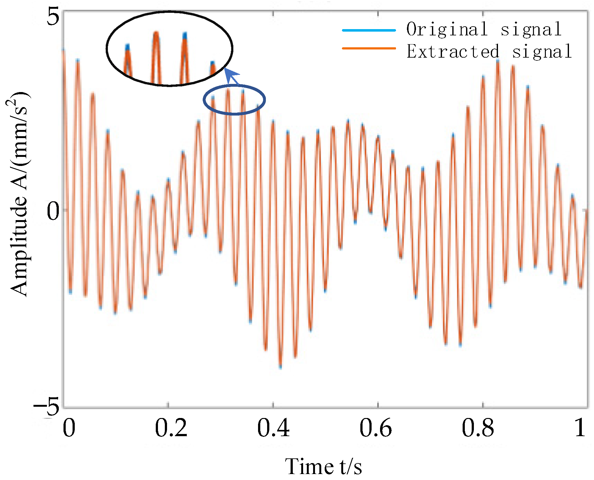
To separate harmonic components, an adaptive orthogonal matching pursuit method (adapOMP) is utilized. Because harmonic and modulation components are scattered on sine waves of specified frequencies, we may compute using the sparse coefficients of these atoms, as shown in Formula (5). Assuming that the maximum value of sparse coefficients obtained after k iterations is a   and the minimum value is b , when a > ρ b , iteration stops outputting sparse coefficients. In order to better recover signals, ρ = 5   can be set through experiments. The final residual signal is the composite signal of impact component and noise.
The harmonic signal can be separated quickly and efficiently by using adaptive orthogonal matching pursuit algorithm. We performed a comparative analysis of different algorithms on signals with specific harmonics and noise added and evaluated the results as Table 1 [34].
The adapOMP has the strongest harmonic extraction ability and less time when it is used alone.
(2)
The improved K-SVD algorithm
A feature extraction approach of learning vocabulary is presented to address the issue that the pre-built lexicon has low flexibility when faced with various forms of failure signals. Dictionary learning may improve the feature information extraction for various fault signal kinds, reducing the interference of extraneous information and enabling the identification of the fault types. The sparse representation solution and dictionary learning are the two crucial elements in the sparse feature extraction approach [35]. To better detect the defect information, we enhance the K-SVD algorithm to optimize the halting criterion of the dictionary learning feature extraction approach.
In order to lessen the sparsity of the sparse coefficient matrix corresponding to the dictionary, the over-complete dictionary learning method K-SVD is suggested. The atoms learnt by K-SVD may then be utilized to reflect the original signal more accurately. The issue can be summarized as follow:
min D , α s D α 2 2   < ε       s . t .       α i 0   T
In the formula, s R m × n represents the original signal, D R m × K represents the dictionary matrix containing K atoms d k , and α R K × n represents the sparse coefficient matrix, where m represents the number of samples and n represents the properties of samples.
The sparse coding and dictionary learning phases of the K-SVD technique are separated. The orthogonal matching pursuit method with enhanced error threshold (OMPerr) is employed in place of the orthogonal matching pursuit algorithm in the sparse representation solution step, and the objective function and constraint conditions of Equation (6) are modified:
min D , α α i 0       s . t .       s i D α i 2 2 ε
The biggest benefit of changing the constraint condition is that the program no longer needs to be stopped by setting the sparsity. It also avoids issues where the original signal cannot be accurately restored due to the sparsity of the sparse coefficient matrix not meeting the precision requirement due to insufficient iterations, as well as issues where the calculation takes too long due to excessive iterations. When the error of the original signal and sparse approximation is less than a predetermined amount, the iteration is halted thanks to the objective function’s error Goal setting, allowing for the accurate form of the signal to be retrieved and a more accurate reconstruction to be produced.
D R m × K , s i R m × 1 , α i R K × 1 s = { s i } i = 1 n , α = { α i } i = 1 n
The meaning of each symbol in Formula (8) is the same as that of the symbol in the Formula (6), where α is the set of solution vectors of s . By resolving the optimization issue in Formula (7) using sparse representation, you may obtain the sparse coefficient vector that corresponds to the initialization dictionary. The dictionary is then updated column by column during the dictionary learning stage using the sparse vectors produced from the sparse coding method. Consider updating the k th atom of the dictionary (designated as d k ) and the k th coefficient of the sparse coefficient matrix (designated as α T k ).
s D α F 2 = s j = 1 K d j α T j F 2 = ( s j k K d j α T j ) d k α T k F 2 = E k d k α T k F 2
where E k = s j k K d j α T j represents the calculation of residual error. In this case, the optimization problem is transformed into:
min d k , α T k E k d k α T k F 2
To obtain the least amount of error, the best d k , α T k solution must be found. This is a least squares issue that can be resolved using the singular value decomposition or the least squares approach (SVD). The SVD approach is employed in this study to find the best possible combination of two variables. Further reducing the computation dimension, the elements in E k and α T k that correspond to zero elements y ( t ) are removed to create a new residual matrix E k .
Using mathematical expressions to describe this step is the sparse coefficient vector is not zero position in 1, the location of the zero element as 0, that is to set up a set of A k = { i | 1 < i < K , α T k ( i ) 0 } to represent the index value when α T k 0 . Define a N× l ( A k ) matrix, B k . The element at position ( A k ( i ) , i ) is 1, and elements at other positions are 0, that is:
E k = E k B k α     T k = α T k B k s k = s k B k
At this point, the target equation can be described as:
min d k , α T k E k d k α     T k F 2
Therefore, to find the best d k , α   T k , we need to perform singular value decomposition of E k .
E k = U Δ V T
The first column u 1 = U ( · , 1 ) of the left singular matrix U is taken as d k , that is, d k = u 1 . Take the product of the first row of the right singular matrix and the first singular value as α   T k , that is, α   T k = Δ ( 1 , 1 ) V T ( 1 , · ) .
Using this technique, one may create a new learning dictionary by replacing each of the columns in the original dictionary. Through this repeated process, the dictionary matrix and coefficient matrix corresponding to the original signal s can be found again and again. The iteration ends if s D α 2 2 < ε .
By improving sparse representation method, harmonic components and part of noise can be well removed, which plays an active role in bearing fault extraction.

2.2. Fault Feature Extraction Based on EEMD

Empirical mode decomposition (EMD) is an adaptive time–frequency localization method, which can be used to analyze and process nonlinear and non-stationary signals [36]. However, EMD also has some shortcomings in the decomposition process. For example, the eigenmode function is easy to produce mode mixing phenomena in the decomposition process, and the signal end effect will also affect the decomposition effect of EMD [37]. EEMD is proposed to improve EMD decomposition, which mainly uses the feature that the mean value of white noise is zero, adding evenly distributed white noise for many times in the decomposition process, covering up the noise of the signal itself by artificially adding white noise, filling up the missing frequency space in the original signal completely, making it continuous in the time-domain, changing the size of extreme points, obtaining a more accurate upper envelope and lower envelope, thus affecting the effect of signal decomposition and further reducing the occurrence of modal aliasing. After many times of average calculation, the influence of noise on the signal is minimized. The more times of calculation, the smaller the influence of noise on the signal.
(1)
EEMD decomposition method
EEMD decomposition is performed on the signal y ( t ) , and   N   groups of different white noises n = [ n 1 ( t ) , n 2 ( t ) , n 3 ( t ) , , n N ( t ) ] are added to the original signal for decomposition. The decomposition process is shown in Table 2:
EEMD decomposes into multiple IMF components, and we need to determine which IMF components are the true components of the signal and which IMF components are the false and meaningless components of the signal. We need to choose the real IMF component to reconstruct the signal, and the remaining IMF components are discarded as meaningless components in the process of reconstructing the signal. However, in order to avoid wrong selection or omission of some real IMF components, we use the correlation coefficient between the original signal and IMF components and the kurtosis value of IMF components as indicators to select real IMF components for signal reconstruction.
The cross-correlation coefficient R c between the real signal y ( i ) and the IMF component x ( i ) is defined as:
ρ j = C o v ( x , y ) s t d ( x ) s t d ( y ) = i = 1 N ( y ( i ) y ( i ) ¯ ) ( x ( i ) x ( i ) ¯ ) i = 1 N ( y ( i ) y ( i ) ¯ ) 2 i = 1 N ( x ( i ) x ( i ) ¯ ) 2
where, ρ j is the correlation coefficient between the real signal and the IMF component, j represents the j th IMF component, i is the data point, N is the signal length, C o v ( x , y ) is the covariance between the real signal and IMF component, and s t d ( x )   and   s t d ( y ) are the standard deviations between the real signal and the IMF component.
In order to select IMF components that are closely related to the original signal for signal reconstruction, a threshold is introduced to limit the selection of IMF components, namely:
T H = 1 n 1 j = 1 n ( ρ j ρ ¯ ) 2
where: n is the number of layers of the original signal decomposed by the EEMD method. In this way, the whole formula becomes the standard deviation of the correlation coefficient between the total IMF component and the original signal. The IMF component larger than T H can be regarded as a real component, otherwise it is regarded as a false component. The real IMF components are selected to extract the transient impact components of each IMF component. After the selected IMF components that are correlated with the original signal, it is also necessary to determine whether the modified components contain obvious impact components. At this time, it is determined whether the component contains an impact component by using the kurtosis value of the calculated signal.
Kurtosis is a dimensionless parameter describing the x distribution characteristics of a signal, which is particularly sensitive to the impact components, and its expression is as follows:
K = 1 n i = 1 N ( x ( i ) x ( i ) ¯ ) 4 s t d ( x )
where n is the number of data points of the signal, x ( i ) ¯ is the average of IMF components, and s t d ( x ) is the standard deviation of the signal.
Generally, it is considered that when the kurtosis value is greater than 3, the shock characteristics of the signal are more obvious. When the kurtosis value is less than 3, the shock characteristic of the signal is not obvious [38]. In order to extract the transient impulse components from IMF components and reconstruct the signals, the IMF components whose cross-correlation coefficient is greater than 0.3 and the kurtosis value is greater than 3, which are correlated with the original signals, are selected for subsequent sparse representation. After sparse denoising, the IMF components are reconstructed to obtain reconstructed signals with rich transient impulse components, and it is easier to judge the fault frequency and fault types of rolling bearings.
(2)
One-dimensional signal folding and hard threshold reconstruction
Through the cross-correlation coefficient and kurtosis value, the IMF component, which contains the impact component and has great correlation with the original signal, is selected for further sparse denoising. Then, the processed IMF components are reconstructed, and then the fault frequency is calculated by the envelope spectrum to judge the fault type.
We need to combine the EEMD algorithm with the K-SVD algorithm to extract fault features. The requirement of K-SVD calculation is that the number of columns of the matrix must be greater than the number of rows of the matrix, that is, the dictionary needs to be an over-complete dictionary. When K-SVD is used to process one-dimensional signals, the signals to be processed can be converted into the Hankel matrix for calculation [39]. The Hankel matrix is a matrix with equal elements on every diagonal line, but the number of columns of the matrix is larger than the number of rows in K-SVD processing, so the Hankel matrix is deformed, that is, the number of elements in each row is larger than that in each column, forming a flat matrix. The IMF component I = [ i 1   i 2   i 3 i n ] is arranged in the Hankel matrix. Namely:
H = H a n k e l ( I ) = [ i 1 i 2 i 3 i K i 2 i 3 i 4 i K + 1 i d i d + 1 i d + 2 i n ] d × K
Dictionary learning requires K to be much greater than d. Sparse representation is carried out with the Hankel matrix containing K signals and each signal dimension of d as input. Each signal contains the information in the original signal, and the latter signal is obtained by the shift of the previous signal, so K signals contain all the information in the original signal. In addition, in the calculation process, each signal needs to be calculated by K-SVD to obtain the learning dictionary and sparse coefficient matrix. The learning dictionary and sparse matrix are multiplied to restore to the form of the Hankel matrix, and the inverse Hankel function is used to restore to the form of one-dimensional signal.
A learning dictionary and the related sparse representation coefficient matrix are generated for each segment of the original signal throughout the signal reconstruction process. The reconstruction signal is then created by multiplying the learning dictionary by the sparse coefficient vector. However, a tiny amount of noise will still perturb the atoms in the learning dictionary. To partially filter out the low-frequency harmonics and noise components, a hard threshold can be implemented. The following optimization issues can be resolved with hard thresholds:
a r g min X X B 2 2 + λ X 0
where X = [ x 1 , x 2 , , x n ] t , B = [ b 1 , b 2 , , b n ] t . X 0 is the zero norm of vector X , and the terms of vector in Equation (18) can be disassembled as:
F ( x ) = X B 2 2 + λ X 0 = [ ( x 1 b 1 ) 2 λ | x 1 | 0 ] + [ ( x 2 b 2 ) 2 λ | x 2 | 0 ] + + [ ( x n b n ) 2 λ | x n | 0 ] = i = 1 n [ ( x i b i ) 2 λ | x i | 0 ]
where | x i | 0 = { 1   , x i 0 0   , x i = 0 , each term in Equation (19) can be written as:
f ( x ) = { ( x b ) 2 + λ           , x 0 b 2                                                   , x = 0
when x 0 , the minimum value of function f ( x ) is obtained at x = b , and the minimum value is λ ; when x = 0 , the value of function f ( x ) is b 2 . In order to get the minimum value, it is necessary to compare the sizes of b 2 and λ . If b 2 > λ , the minimum value of the function is obtained at x = b ; If b 2 < λ the minimum value of the function is obtained at x = 0 . That is:
a r g m i n f ( x ) = { 0     | b | < λ b     | b | > λ
b is regarded as a variable, is regarded as a threshold, and Formula (21) is a hard threshold. The optimization problem of Formula (18) can be written as follows:
X = h a r d ( B , λ ) = { 0     | B | < λ B     | B | > λ
Use all the elements in vector B , compare with the threshold, discard the elements less than the threshold, and keep the elements greater than the threshold. When B is a matrix, this formula can still be used, and each element in the formula is compared with the threshold to make a choice. A more intuitive function image is used to represent the hard threshold function. Let the function y = x , x [ 3 , 3 ] and the threshold value be 1. The image is shown in Figure 1. All the function values whose absolute value is less than the threshold value are discarded, and the function values whose absolute value is greater than the threshold value are retained.
After the original signal is divided and converted into the Hankel matrix, the learning dictionary matrix and sparse coefficient vector are obtained by K-SVD calculation. However, due to the influence of noise, the atoms of learning dictionary will still be affected by some noise. Using the hard threshold denoising method to remove smaller elements in dictionary atoms and further eliminate noise interference, the learning dictionary optimization model can be obtained as follow:
a r g min D 1 D 1 D 2 2 + λ D 1 0
By setting a hard threshold to further eliminate noise interference, the optimized dictionary D 1 is obtained. Usually, there are two ways to set the threshold. One is to debug through conventional artificial experiments, check the output results, and select the optimal threshold value. The second is to look for an index of the signal to choose, such as the signal-to-noise ratio of the noise-reduced signal as an index, and then set the corresponding threshold to the optimal value when the signal-to-noise ratio is the maximum. Through a series of tests, the threshold is set to 0.2 in this paper to further optimize the learning dictionary. Use the optimized dictionary to reconstruct the signal, that is:
H = D 1 x = [ i 1 i 2 i 3 i K i 2 i 3 i 4 i K + 1 i d i d + 1 i d + 2 i n ] d × K
The reconstructed Hankel matrix is transformed into a one-dimensional signal, and several pieces of signals are merged together to restore the original signal. At this time, the signal with K-SVD denoising is obtained. The envelope spectrum analysis is carried out to determine the fault frequency of rolling bearing and judge the fault type of rolling bearing.
Combined with the hard threshold denoising EEMD and sparse representation method, the capability of fault feature extraction is further improved.

3. Bearing Fault Feature Extraction Method Based on Improved Sparse Representation and EEMD Algorithm

The process of the bearing fault feature extraction method based on improved sparse representation and EEMD algorithm can be divided into three stages:
Stage 1: Preprocess and separate the mixed harmonic signals in the original signal by using the adapOMP algorithm combined with the Fourier dictionary.
Stage 2: Combined with hard threshold denoising, the signals of the previous stage are decomposed by the EEMD algorithm, and the selected IMF components are transformed by the Hankel matrix to build the initial learning dictionary.
Stage 3: Finally, the signal is processed by the K-SVD algorithm with improved termination criterion.
Finally, the signal with obvious fault characteristics can be obtained through signal reconstruction.
Details are shown in Figure 2.

4. Signal Simulation Analysis

Construct a composite signal composed of harmonics and their modulation components, transient impact components, and noise, and its mathematical expression is:
{ y ( t ) = k h ( t T 0 k T ) + s ( t ) + n ( t ) h ( t ) = e α t sin ( 2 π f z t ) ( sin ( 2 π f r t ) + C ) s ( t ) = cos ( 2 π × 3.5 t ) + ( 2 + cos ( 2 π × 2.5 t ) ) cos ( 2 π × 35 t )
The transient impact component is h ( t ) , the harmonic and its modulation component is s ( t ) , and the noise component is n ( t ) . The initial fault location is 0.026 s, the fault period is 0.1 s, and the fault frequency is 10 Hz. The attenuation index is α = 1200 , the natural frequency f z is 2000 Hz, the sampling frequency f r is 2000 Hz, the sampling time is 1 s, and the number of sampling points is 2000. Add Gaussian white noise with a mean value of 0, a variance of 1, and an amplitude of 0.25. The time-domain waveform is shown in Figure 3.
First, randomly build a 2000 × 4000 Fourier frequency dictionary, and use the adaptive orthogonal matching pursuit algorithm to eliminate harmonics and their modulation components in the coincidence signal, and get the sparsity of five, which appears at the atomic position and the sparsity coefficient as shown in Table 3. Comparing the extracted harmonic components with the original harmonic components, as shown in Figure 4, red represents the harmonic components, and blue represents the harmonic components removed from the composite signal, with a cross-correlation coefficient of 0.9992. The harmonic and its modulation components can basically be removed from the original signal, that is, only transient pulse components and noise are left in the original signal. As shown in Figure 5.
The adaptive orthogonal matching pursuit algorithm is used to eliminate harmonics and their modulation components, and the coincidence signal of transient impact components and noise is obtained. Then, the obtained one-dimensional signal is converted into the Hankel matrix. When using the K-SVD algorithm, the number of columns of the matrix is much larger than the number of rows of the matrix. If the matrix is too large, the calculation speed of K-SVD will be affected. If the matrix is too large, the algorithm will not converge, and the desired result will not be obtained. Therefore, how to design the ratio of rows to columns in the Hankel matrix and how to segment long signals are discussed to find the best signal conversion and segmentation results. Take the simulation signal in this section as an example: the signal length is 2000, and the number of rows and columns of the Hankel matrix is equal to the signal length plus 1, because the K-SVD algorithm requires that the number of rows of signals is less than the number of columns. By changing the ratio of rows to columns, the size of the Hankel matrix is changed, and the representative rows of 100 and integer multiples of 100 are selected for display until 1000 rows. The kurtosis and signal-to-noise ratio of K-SVD denoised signal are calculated to determine the optimal ratio of rows and columns for Hankel. It is determined that the number of training atoms is 1000 without changing, and the number of iterations is 10 times. The initial dictionary is obtained by processing the original signal. Based on the statistical calculation time of Intel(R) Core(TM) i5-6300HQ CPU @ 2.30 GHz 2.30 GHz laptop, the obtained denoising effect is shown in Figure 6. And Figure 6a–e are time-domain waveforms of Hankel matrix after denoising by K-SVD algorithm when the number of rows is respectively 200, 400, 600, 800 and 1000. The time-domain waveform of the Hankel matrix after denoising by the K-SVD algorithm can be calculated by many experiments, and the fitting curve between the ratio of rows and columns of the Hankel matrix and the kurtosis value can be obtained as shown in Figure 7. The data of some points are shown in Table 4, and the best denoising effect can be obtained when the ratio of rows and columns of the Hankel matrix is one quarter, and the calculation time changes with the increase in rows.
In actual signals, the number of sampling points is often large and the signal length is long. If it is directly converted into the Hankel matrix, the matrix will be too large, which will lead to too long a calculation time and even lead to non-convergence of the algorithm. Next, consider the influence of subsection calculation on the algorithm. According to the simulation signal, 2000 data points are divided into four groups of control experiments, including one segment, two segments, four segments, and five segments. It is determined that the ratio of rows and columns of the Hankel matrix in each segment is 1 to 4. When running the K-SVD algorithm, the number of trained dictionary atoms is twice the number of rows of the Hankel matrix, and the time-domain waveform of its de-noising signal is shown in Figure 8a–d. The specific data of the time-domain waveforms of the denoised signals in segments four and five are shown in Table 5. By calculating the kurtosis value and the signal-to-noise ratio, it can be seen that when the original signal is divided into four segments, that is, 500 data points in each segment are calculated, a better denoising effect can be obtained, and the calculation time can be greatly shortened. In the long signal processing, we can divide the original signal into 500 data points and transform it into a Hankel matrix of 100 × 401 size for K-SVD denoising, which can improve the accuracy of signal reconstruction, shorten the calculation time, and better identify the fault type.
After many experiments, the signal decomposition scheme is determined as 500 data points per segment, which is transformed into a 100 × 401 Hankel matrix for K-SVD decomposition, and the segmented orthogonal matching pursuit algorithm and hard threshold algorithm are used to further denoise the signal. EEMD pre-denoise the signal excluding harmonic components, setting the added noise amplitude to be 0.25 and the lumped average times to be 1000 times. The IMF components after EEMD decomposition are shown in Figure 9, showing only the first eight layers. The kurtosis values of IMF1-IMF8 components and the correlation coefficients with the original signals are shown in Table 6.
By calculating the standard deviation of the correlation coefficient of the IMF component, the threshold value is 0.2478, only the correlation coefficients of the IMF1 component and the IMF2 component with the original signal are greater than this threshold value, and the kurtosis values of the IMF1 component and the IMF2 component are both greater than 3.0, which indicates that the IMF1 component and the IMF2 component have great correlation with the filtered signal and contain rich impact components, so the IMF1 component and the IMF2 component are selected for sparse denoising. The hard threshold coefficient is determined to be 0.2 through many artificial experiments. The time-domain waveforms of the IMF1 component and the IMF2 component before and after denoising are shown in Figure 10 and Figure 11. All the transient impact components in the original signal have been preserved, and most of the noise components have been eliminated. The signals after sparse denoising of the IMF1 component and the IMF2 component are reconstructed to obtain the reconstructed signal, as shown in Figure 12, and the envelope spectrum analysis of the reconstructed signal is shown in Figure 13.
There is almost no clutter in the envelope spectrum of the reconstructed signal; which shows that its noise and harmonic components are clear and clean, and the 15th harmonic or even more of the fault frequency can be clearly observed, which is enough to show that this method has a good suppression effect on harmonic components and noise when extracting transient impact components.

5. Experimental Verification and Analysis

The gearbox dynamics simulator (GDS) produced by Spectra Quest of the United States was employed to build the experimental platform and simulate the data. After the data is collected, it would be analyzed by the algorithm in this paper in order to further confirm the efficacy of the approach suggested in this study in isolating transient impact components against a significant noise background. The signal acquisition device, motor, gear box, and load device are the four components that make up the testbed. The signal acquisition instrument and a piezoelectric sensor make up the acquisition equipment. A power unit is made up of the motor, a 3 HP three-phase asynchronous motor with a maximum speed of 5000 rpm, a rotary speed controller, and various display devices. In Figure 14, the test bench is seen.
Using a HG-8916 data acquisition system, the maximum sampling number of the signal acquisition card is 32,768, and the maximum sampling frequency is 50 kHz, which is saved in .txt format and imported into MATLAB for analysis. During the experiment, due to the limitation of conditions, acceleration sensors can only be installed outside the gear box to collect vibration data. Sensors are installed at seven positions in total, and their installation positions and measuring points are shown in Figure 15. Among them, piezoelectric acceleration sensors are installed at measuring points P1 to P6 to collect vibration data, and laser speed sensors are installed at measuring point P7 to measure motor speed. The experimental bearing is a ER-16K deep groove ball bearing, which supports the input shaft at the driving end. The bearing parameters are shown in Table 7.
In this experiment, the sampling frequency is 20 kHz, the motor frequency is 23.5 Hz, the acquisition time is 1 s, and there are 20,000 data points in total. According to the bearing data, 83.94 Hz is the outer ring fault frequency. A total of 10,000 data points within 0.5 s are intercepted for analysis in this part, and Figure 16 displays the time-domain waveform and its envelope spectrum. The transient impact component is completely masked by the strong background noise and harmonic components, as can be seen from the time-domain waveform, and only the fault characteristic frequency of its second harmonic frequency can be seen in the envelope spectrum. As a result, it is challenging to determine the type of bearing fault because all other harmonic frequencies are completely masked by the high-frequency harmonic components and noise. In this paper, a method is presented for separating the transient pulse components from the original signal and determining the various rolling bearing fault types.
First, the harmonic and modulation components are separated using the adaptive orthogonal matching pursuit technique, and a 10,000 × 20,000 entry over-complete Fourier dictionary is created. The sparsity is six, and it could be found at the atoms of the six Fourier dictionaries, which are, in order, the 39th, 77th, 6998th, 7036th, 16,323rd, and 16,361st. The original signal is filtered to remove harmonics and low-frequency noise, and Figure 17 displays the resulting signal. The adaptive orthogonal matching pursuit technique has removed most of the harmonic signals from the original signal, progressively revealing the transient impact component. Then, two approaches are compared. One is to use the K-SVD algorithm with an improved termination criterion for noise reduction, the other is to combine the EEMD algorithm with the K-SVD algorithm for noise reduction, and the results are compared.
The filtered signal is decomposed by EEMD, and the amplitude of added white noise is set at 0.25, and the lumped average times are 1000 times. The results of the IMF components in the first eight layers are shown in Figure 18, and the results of cross-correlation coefficient and kurtosis between each IMF component and the original signal are shown in Table 8.
By calculating the standard deviation of the first eight decomposed IMF components, the threshold value is set at 0.2444; that is, IMF components with correlation coefficients greater than this threshold value are regarded as real components. In Table 8, the correlation coefficients of the three components of IMF1, IMF2, and IMF3 with filtered signals are all greater than the set threshold value, indicating that these three components have a strong correlation with filtered signals, and their kurtosis is greater than 3.0, which contains obvious impact components. Therefore, IMF1, IMF2, IMF3 are selected. Each IMF component contains 10,000 data points, which are divided into 20 segments with 500 data points in each segment and converted into a Hankel matrix of 100 × 401 for K-SVD denoising. The number of atoms trained in each segment is 200, and finally the hard threshold is set at 0.2. The result is shown in Figure 18.
Sparse denoising is performed on the IMF1, IMF2, and IMF3 components, and the time-domain waveforms before and after denoising are shown in Figure 19, Figure 20 and Figure 21, respectively. In the time-domain waveform diagram of the IMF component denoising, we can see that most of the noise has been removed, and the periods of each transient impact component are obvious, and there is basically no noise interference between every two periods. The signals after sparse denoising of IMF1, IMF2, and IMF3 are reconstructed to obtain the reconstructed signal as shown in Figure 22e, and the envelope spectrum of the reconstructed signal is shown in Figure 22f. From the envelope spectrum of the reconstructed signal, it can be seen that the fault frequency and its frequency doubling of the rolling bearing are obvious, and the interference of harmonics and their modulation components and noise components is small.
Three methods are used to analyze the same signal and the results are compared. Through direct time-domain analysis and frequency-domain analysis, the fault components in bearing operations can be preliminarily found, but it is only sensitive to the step signal of one frequency (Figure 22a,b). Further, the adapOMP algorithm is used to filter the signal, and the K-SVD algorithm with improved termination criteria is used to analyze the filtered signal shown in Figure 22c. It can be seen that the fault characteristics of the bearing can be clearly displayed, but the processing ability for low-frequency signals is still weak (Figure 22d). Furthermore, this paper purposely selects hard threshold denoising to process low-frequency harmonics and noise in the signal. The reconstructed signal is shown in Figure 22e and further analyzed by the EEMD algorithm. The final frequency-domain envelope spectrum is shown in Figure 22f. Compared with the first two methods, this method expands the available range of fault identification

6. Conclusions

In this paper, aiming at the problem that it is difficult to extract rolling bearing faults online, a bearing fault feature extraction method based on the EEMD algorithm and improved spare representation is proposed, Firstly, an adaptive OMP (adapOMP) algorithm and K-SVD algorithm with improved termination criteria are proposed, thus forming an improved sparse representation method. In some cases, the improved sparse representation method can already extract some fault features, but the effect is not good in a low-frequency range. Therefore, combining the improved sparse representation method with the EEMD method of hard threshold denoising can well separate the fault features in simulation and experimental verification. The main features of this algorithm are:
(1)
By constructing a Fourier dictionary, the OMP algorithm is improved to make it more adaptive to harmonic signals.
(2)
The decomposition results of EEMD are processed by hard threshold denoising, which solves the problem that the IMF component is not obvious.
(3)
The K-SVD algorithm is improved with OMPerr. After the improvement, the algorithm automatically selects the sparsity with the best performance without manual selection, which improves the efficiency and accuracy of algorithm processing.
This method improves the shortcomings of the previous methods that are insensitive to low-frequency signals and broadens the scope of application of the algorithm. However, although we strive to improve the algorithm to make it as adaptive as possible to reduce the number of its parameter settings, thereby reducing the influence of the operator’s knowledge level on the applicability of the algorithm, there are still some parameter settings that depend on experience. In the future, the end-to-end data-driven approach or the model-data-fusion driven approach may further address this issue.

Author Contributions

Conceptualization, L.W., D.X. (Da Xu) and C.C.; methodology, X.L. and D.X. (Da Xu); software, D.X. (Da Xu); validation, X.L., D.X. (Da Xu), S.A. and C.W.; formal analysis, D.X. (Da Xu); investigation, D.X. (Da Xu) and C.W.; resources, L.W., S.A. and C.C.; data curation, D.X. (Da Xu) and C.W.; writing—original draft preparation, X.L., and D.X. (Da Xu); writing—review and editing, X.L. and D.X. (Donglai Xu); visualization, X.L., D.X. (Da Xu) and D.X. (Donglai Xu); supervision, L.W. and C.C.; project administration, L.W. and C.C.; funding acquisition, L.W. and C.C. All authors have read and agreed to the published version of the manuscript.

Funding

This research was supported by the National Natural Science Foundation of China Youth Fund, grant number 62003315; Scientific and Technological Project of Henan Province, grant number 212102210069; Henan Province “ZHONGYUAN Thousand Talent Program”, grant number ZYQR201810075; ZHONGYUAN Talent Program, grant number ZYYCYU202012112; Zhengzhou Measurement and Control Technology and Instrument Key Laboratory, grant number 121PYFZX181; the Applied Basic Research Program of Shanxi Province, grant number 201901D211241; and The Young Academic Leaders Support Program of the North University of China, grant number QX202002.

Institutional Review Board Statement

Not applicable.

Informed Consent Statement

Not applicable.

Data Availability Statement

The data involved in this article have been presented in the article.

Conflicts of Interest

The authors declare no conflict of interest.

References

  1. Jia, F.; Lei, Y.G.; Lin, J.; Zhou, X.; Lu, N. Deep neural networks: A promising tool for fault characteristic mining and intelligent diagnosis of rotating machinery with massive data. Mech. Syst. Signal Proc. 2016, 72–73, 303–315. [Google Scholar] [CrossRef]
  2. Zhang, X.; Liu, Z.W.; Miao, Q.; Wang, L. Bearing fault diagnosis using a whale optimization algorithm-optimized orthogonal matching pursuit with a combined time-frequency atom dictionary. Mech. Syst. Signal Proc. 2018, 107, 29–42. [Google Scholar] [CrossRef]
  3. Ben Ali, J.; Fnaiech, N.; Saidi, L.; Chebel-Morello, B.; Fnaiech, F. Application of empirical mode decomposition and artificial neural network for automatic bearing fault diagnosis based on vibration signals. Appl. Acoust. 2015, 89, 16–27. [Google Scholar] [CrossRef]
  4. Tian, J.; Ai, Y.T.; Fei, C.W.; Zhang, F.L.; Choy, Y.S. Dynamic modeling and simulation of inter-shaft bearings with localized defects excited by time-varying displacement. J. Vib. Control 2019, 25, 1436–1446. [Google Scholar] [CrossRef]
  5. El-Thalji, I.; Jantunen, E. A summary of fault modelling and predictive health monitoring of rolling element bearings. Mech. Syst. Signal Proc. 2015, 60–61, 252–272. [Google Scholar] [CrossRef]
  6. Niu, L.K.; Cao, H.R.; Hou, H.P.; Wu, B.; Lan, Y.; Xiong, X.Y. Experimental observations and dynamic modeling of vibration, characteristics of a cylindrical roller bearing with roller defects. Mech. Syst. Signal Proc. 2020, 138, 19. [Google Scholar] [CrossRef]
  7. Yu, G. A Concentrated Time-Frequency Analysis Tool for Bearing Fault Diagnosis. IEEE Trans. Instrum. Meas. 2020, 69, 371–381. [Google Scholar] [CrossRef]
  8. Wang, L.M.; Shao, Y.M. Fault feature extraction of rotating machinery using a reweighted complete ensemble empirical mode decomposition with adaptive noise and demodulation analysis. Mech. Syst. Signal Proc. 2020, 138, 20. [Google Scholar] [CrossRef]
  9. Zvokelj, M.; Zupan, S.; Prebil, I. EEMD-based multiscale ICA method for slewing bearing fault detection and diagnosis. J. Sound Vibr. 2016, 370, 394–423. [Google Scholar] [CrossRef]
  10. Tian, J.; Liu, L.L.; Zhang, F.L.; Ai, Y.T.; Wang, R.; Fei, C.W. Multi-Domain Entropy-Random Forest Method for the Fusion Diagnosis of Inter-Shaft Bearing Faults with Acoustic Emission Signals. Entropy 2020, 22, 15. [Google Scholar] [CrossRef] [Green Version]
  11. Ai, Y.T.; Guan, J.Y.; Fei, C.W.; Tian, J.; Zhang, F.L. Fusion information entropy method of rolling bearing fault diagnosis based on n-dimensional characteristic parameter distance. Mech. Syst. Signal Proc. 2017, 88, 123–136. [Google Scholar] [CrossRef]
  12. Li, X.; Zhang, W.; Ding, Q. Deep learning-based remaining useful life estimation of bearings using multi-scale feature extraction. Reliab. Eng. Syst. Saf. 2019, 182, 208–218. [Google Scholar] [CrossRef]
  13. He, Z.Y.; Shao, H.D.; Jing, L.; Cheng, J.S.; Yang, Y. Transfer fault diagnosis of bearing installed in different machines using enhanced deep auto-encoder. Measurement 2020, 152, 13. [Google Scholar]
  14. Hou, M.W.; Wang, W.Y. Sensor Mathematical Model Data Fusion Biobjective Optimization. J. Sens. 2022, 2022, 1612715. [Google Scholar] [CrossRef]
  15. Li, T.M.; Si, X.S.; Pei, H.; Sun, L. Data-model interactive prognosis for multi-sensor monitored stochastic degrading devices. Mech. Syst. Signal Proc. 2022, 167, 24. [Google Scholar] [CrossRef]
  16. Zhou, T.T.; Te, H.; Droguett, E.L. Towards trustworthy machine fault diagnosis: A probabilistic Bayesian deep learning framework. Reliab. Eng. Syst. Saf. 2022, 224, 13. [Google Scholar] [CrossRef]
  17. Wang, Y.X.; Xiang, J.W.; Markert, R.; Liang, M. Spectral kurtosis for fault detection, diagnosis and prognostics of rotating machines: A review with applications. Mech. Syst. Signal Proc. 2016, 66–67, 679–698. [Google Scholar] [CrossRef]
  18. Verstraete, D.; Ferrada, A.; Droguett, E.L.; Meruane, V.; Modarres, M. Deep Learning Enabled Fault Diagnosis Using Time-Frequency Image Analysis of Rolling Element Bearings. Shock Vib. 2017, 2017, 5067651. [Google Scholar] [CrossRef]
  19. Tian, J.; Wang, S.G.; Zhou, J.; Ai, Y.T.; Zhang, Y.W.; Fei, C.W. Fault Diagnosis of Intershaft Bearing Using Variational Mode Decomposition with TAGA Optimization. Shock Vib. 2021, 2021, 8828317. [Google Scholar] [CrossRef]
  20. Xuan, B.; Xie, Q.W.; Peng, S.L. EMD sifting based on bandwidth. IEEE Signal Process. Lett. 2007, 14, 537–540. [Google Scholar] [CrossRef]
  21. Lei, Y.G.; He, Z.J.; Zi, Y.Y. Application of the EEMD method to rotor fault diagnosis of rotating machinery. Mech. Syst. Signal Proc. 2009, 23, 1327–1338. [Google Scholar] [CrossRef]
  22. Lei, Y.G.; He, Z.J.; Zi, Y.Y. EEMD method and WNN for fault diagnosis of locomotive roller bearings. Expert Syst. Appl. 2011, 38, 7334–7341. [Google Scholar] [CrossRef]
  23. Liu, D.; Zeng, H.T.; Xiao, Z.H.; Peng, L.H.; Malik, O.P. Fault diagnosis of rotor using EMD thresholding-based de-noising combined with probabilistic neural network. J. Vibroeng. 2017, 19, 5920–5931. [Google Scholar]
  24. Mohanty, S.; Gupta, K.K.; Raju, K.S. Hurst based Vibro-Acoustic Feature Extraction of Bearing using EMD and VMD. Measurement 2017, 117, 200–220. [Google Scholar] [CrossRef]
  25. Wang, J.; Du, G.F.; Zhu, Z.K.; Shen, C.Q.; He, Q.B. Fault diagnosis of rotating machines based on the EMD manifold. Mech. Syst. Signal Proc. 2020, 135, 21. [Google Scholar] [CrossRef]
  26. Liu, D.; Xiao, Z.H.; Hu, X.; Zhang, C.X.; Malik, O.P. Feature extraction of rotor fault based on EEMD and curve code. Measurement 2019, 135, 712–724. [Google Scholar] [CrossRef]
  27. Hsieh, N.K.; Lin, W.Y.; Young, H.T. High-Speed Spindle Fault Diagnosis with the Empirical Mode Decomposition and Multiscale Entropy Method. Entropy 2015, 17, 2170–2183. [Google Scholar] [CrossRef]
  28. Wang, C.S.; Sha, C.Y.; Su, M.; Hu, Y.K. An algorithm to remove noise from locomotive bearing vibration signal based on self-adaptive EEMD filter. J. Cent. South Univ. 2017, 24, 478–488. [Google Scholar] [CrossRef]
  29. Liu, J.; Wang, L.F.; Tan, H.J.; Wang, L.M.; Chen, Z.G.; Shao, Y.M. An Extended EEMD Method for Localized Faults Detection of a Planetary Gearbox. J. Test. Eval. 2019, 47, 758–774. [Google Scholar] [CrossRef]
  30. Li, H.; Bu, S.Q.; Wen, J.R.; Fei, C.W. Synthetical Modal Parameters Identification Method of Damped Oscillation Signals in Power System. Appl. Sci. 2022, 12, 21. [Google Scholar] [CrossRef]
  31. Xing, Z.; Lin, J.H.; Huang, Y.; Yi, C. A Feature Extraction Method of Wheelset-Bearing Fault Based on Wavelet Sparse Representation with Adaptive Local Iterative Filtering. Shock Vib. 2020, 2020, 2019821. [Google Scholar] [CrossRef]
  32. He, G.L.; Ding, K.; Lin, H.B. Fault feature extraction of rolling element bearings using sparse representation. J. Sound Vibr. 2016, 366, 514–527. [Google Scholar] [CrossRef]
  33. Tong, Q.B.; Sun, Z.L.; Nie, Z.W.; Lin, Y.Y.; Cao, J.C. Sparse decomposition based on ADMM dictionary learning for fault feature extraction of rolling element bearing. J. Vibroeng. 2016, 18, 5204–5216. [Google Scholar] [CrossRef]
  34. Wang, L.J.; Li, X.Y.; Xu, D.; Ai, S.J.; Wang, C.G.; Chen, C.X. Bearing Fault Feature Extraction Based on Adaptive OMP and Improved K-SVD. Processes 2022, 10, 23. [Google Scholar] [CrossRef]
  35. Zeng, M.; Chen, Z. Iterative K-Singular Value Decomposition for Quantitative Fault Diagnosis of Bearings. IEEE Sens. J. 2019, 19, 9304–9313. [Google Scholar] [CrossRef]
  36. Yeh, J.R.; Sun, W.Z.; Shieh, J.S.; Huang, N.E. Intrinsic Mode Analysis of Human Heartbeat Time Series. Ann. Biomed. Eng. 2010, 38, 1337–1344. [Google Scholar] [CrossRef]
  37. Lee, D.H.; Ahn, J.H.; Koh, B.H. Fault Detection of Bearing Systems through EEMD and Optimization Algorithm. Sensors 2017, 17, 16. [Google Scholar] [CrossRef]
  38. Qiang, M.; Dong, W. Fast Bayesian Inference on Optimal Wavelet Parameters for Bearing Fault Diagnosis. In Proceedings of the ASME 2015 International Mechanical Engineering Congress and Exposition, Houston, TX, USA, 13–19 November 2015. [Google Scholar]
  39. Sun, W.F.; Zhou, Y.Q.; Xiang, J.W.; Chen, B.Q.; Feng, W. Hankel Matrix-Based Condition Monitoring of Rolling Element Bearings: An Enhanced Framework for Time-Series Analysis. IEEE Trans. Instrum. Meas. 2021, 70, 10. [Google Scholar] [CrossRef]
Figure 1. Hard threshold denoising.
Processes 10 01734 g001
Figure 2. Signal processing flow combining EEMD and sparse representation algorithms.
Processes 10 01734 g002
Figure 3. Synthetic signal time-domain waveform. (a) Harmonic components; (b) Impact component; (c) Noise; and (d) Synthetic signal.
Processes 10 01734 g003
Figure 4. Comparison of harmonic components extracted by adapOMP algorithm and original harmonic components.
Processes 10 01734 g004
Figure 5. Filtered signal time-domain waveform.
Processes 10 01734 g005
Figure 6. Hankel matrix transformation test. (a) 200 lines; (b) 400 lines; (c) 600 lines; (d) 800 lines; and (e) 1000 lines.
Processes 10 01734 g006
Figure 7. The fitted curve between the ratio of the number of rows and columns of the Hankel matrix and the kurtosis value.
Processes 10 01734 g007
Figure 8. Hankel matrix segmentation test. (a) 1 segment; (b) 2 segments; (c) 4 segments; and (d) 5 segments.
Processes 10 01734 g008
Figure 9. EEMD decomposition results of simulated signals.
Processes 10 01734 g009
Figure 10. IMF1 denoising result.
Processes 10 01734 g010
Figure 11. IMF2 denoising result.
Processes 10 01734 g011
Figure 12. Time-domain waveform of reconstructed signal.
Processes 10 01734 g012
Figure 13. The envelope spectrum of the reconstructed signal.
Processes 10 01734 g013
Figure 14. Gearbox experimental platform.
Processes 10 01734 g014
Figure 15. Sensor measuring point location.
Processes 10 01734 g015
Figure 16. Time-domain waveform and envelope spectrum of signal of the test bearing.
Processes 10 01734 g016
Figure 17. Filtered signal time-domain waveform after adapOMP.
Processes 10 01734 g017
Figure 18. EEMD decomposition results.
Processes 10 01734 g018
Figure 19. IMF1 denoising result.
Processes 10 01734 g019
Figure 20. IMF2 denoising result.
Processes 10 01734 g020
Figure 21. IMF3 denoising result.
Processes 10 01734 g021
Figure 22. Signal processing results of different methods. (a) Direct time-domain analysis of signals; (b) Direct frequency domain analysis of signals; (c) Time-domain analysis of signals using improved sparse representation algorithm; (d) Frequency-domain analysis of signals using improved sparse representation algorithm; (e) Time-domain analysis of the signal using the algorithm in this paper; and (f) Frequency domain analysis of the signal using the algorithm in this paper.
Processes 10 01734 g022
Table 1. Performance of different methods to extract harmonic components.
adapOMPWaveletEEMD
Accuracy0.98990.72180.9684
Time/s2.293110.6067362.10588
Table 2. EEMD decomposition process.
EEMD algorithm
Input: Original signal y(t), number of original signal processing times N , number of iterations i = 0;
Step 1: Adding white noise to the original signal y ( t ) to obtain y 1 ( t ) ;
                                                                 y 1 ( t ) = y ( t ) + n 1 ( t )
Step 2: EMD decomposition of the noised signal was performed to obtain K IMF components and residual components.
1.
Let r 0 ( t ) = y 1 ( t ) ; a = 0;
2.
Calculate the a th IMF component;
Initialize h 0 ( t ) = r a 1 ( t ) , j = 1;
Find out the local extreme point of h j 1 ( t ) ;
The maximum and minimum points of h j 1 ( t ) are interpolated by cubic spline function to form the upper envelope and the lower envelope;
Calculate the average of the upper and lower envelopes m j 1 ( t ) ;
h j ( t ) = h j 1 ( t ) m j 1 ( t ) ;
Judge whether h j ( t )   meets the conditions of IMF, if so, I M F j ( t ) = h j ( t ) ; If not, j = j + 1 and continue the steps ②–⑥;
3.
Separate IMF component I M F a from signal r a 1 ( t ) to obtain residual signal r a ( t ) , r a ( t ) = r a 1 ( t ) I M F a ( t ) ;
4.
Judging whether the residual signal is less than a given threshold, if it is less than the given threshold, stopping iteration and outputting IMF components; if no, a = a + 1 , repeat 2–4 steps until the residual signal is less than the given threshold. Finally, the following can be acquired:
  •                                                                          y 1 ( t ) = k = 1 K I M F i k + r i k
Step 3: Let i = i + 1, repeat steps 2 to 3 until i = N;
Step 4: Calculate the IMF component obtained by EEMD decomposition d k .
                                                     d k = 1 N i = 1 N I M F i k
Table 3. Sparse representation coefficients of different atoms.
Number of AtomsThe number of columns of atomsSparse Coefficient
NO. 1832.1725
NO. 26615.9327
NO. 37163.0780
NO. 47616.0119
NO. 525213.1795
Table 4. Running results of K-SVD denoising with different row and column numbers of Hankel matrix.
Number of Rows of Hankel MatrixKurtosis ValueSNR/dBComputation Time/s
10015.31534.014850.4658
20017.87914.339153.2103
30018.51674.170763.8960
40021.84184.766171.1505
50019.28483.618580.7429
60018.67054.033189.7161
70016.47953.079397.4496
80015.50611.7097115.3987
90014.84281.9012123.7318
100010.96890.2762131.8154
Table 5. Running results of K-SVD denoising with different number of segments of Hankel matrix.
Number of Rows of SegmentsKurtosis ValueSNR/dBComputation Time/s
124.84184.766163.8960
214.24763.043416.6846
423.26204.94596.3514
521.38814.74736.4313
Table 6. Correlation coefficients of IMF components of simulated signals and their kurtosis indexes.
Correlation CoefficientKurtosis Value
IMF10.79736.6059
IMF20.41274.1886
IMF30.22393.3812
IMF40.18403.2547
IMF50.15003.0936
IMF60.10382.7075
IMF70.07863.0126
IMF80.05502.3138
Table 7. Test bearing specific parameters.
ProjectsParameters
Bearing DesignationER-166K
Pitch diameter D / m m 38.506
Rolling elements diameter d / m m 8.006
Number of rolling bodies9
Contact angle β / ° 0
Fault typePitting of bearing outer ring
Table 8. Correlation coefficients of IMF components of simulated signals and their kurtosis indexes.
Correlation CoefficientKurtosis Value
IMF10.79003.3974
IMF20.50044.5938
IMF30.35664.0362
IMF40.21152.9451
IMF50.15023.1064
IMF60.10452.7361
IMF70.09985.2383
IMF80.13743.4804
Publisher’s Note: MDPI stays neutral with regard to jurisdictional claims in published maps and institutional affiliations.

