KPLS-Based Mach Number Prediction for Multi-Mode Wind Tunnel Flow System

Abstract

In wind tunnels, the Mach number needs to be precisely monitored and controlled. It is difficult to obtain the Mach number directly online, especially when the wind tunnel system is operating in multiple modes. To deal with this problem, a Mach number prediction algorithm based on the kernel partial least squares method is proposed for multi-mode wind tunnel systems. First, in order to reflect real-time changes, the time-slice partial least squares regression method is adopted. Then, in order to enable the model to represent information about the whole working mode divided by key process variables, the mean-value partial least squares model is established and is compared with the time-slice model. Then, considering that wind tunnel systems exhibit strong nonlinear characteristics, the kernel partial least squares method, which is suitable for nonlinear systems, is used to predict the Mach number. The results show that the mean-value model is better than the time-slice model, the models for single modes show better prediction abilities than those for multiple modes, and the kernel partial least square method is more suitable for wind tunnel systems than the partial least square method.

1. Introduction

Wind tunnels use power devices to drive controllable air flow in an annular pipe designed according to certain requirements in order to carry out various aerodynamic tests according to the relativity and similarity principle of motion [1].

Wind tunnel systems are essential for the research and design of aircraft. They are also a requirement for the space industry and their use contributes significantly to scientific developments [2]. With the emergence of various new aerospace vehicles, the requirements of wind tunnel tests are increasing day by day. The wind tunnel has become the most important piece of test equipment for the study of the aerodynamic characteristics of aircraft. During wind tunnel system operation, the Mach number is a key performance index; its stability has an important influence on the quality of the wind tunnel flow field. Thus, many suggestions have been put forward on how to control this variable in a wind tunnel system. If the control operation is appropriate, not only are the experimental results more accurate, but costs can also be reduced and resources can be saved. This indicates the need to be able to make fast and accurate predictions of the Mach number. In addition, a high degree of Mach number accuracy is required in simulated aircraft flights. According to standards in the field of aerodynamics, the control accuracy of the Mach number should be limited to ±0.001 [3,4]. If the prediction accuracy of the Mach number does not meet this requirement, the control accuracy will be reduced, which will have an adverse effect on the wind tunnel experimental process. Therefore, scientific research on Mach number predictions in wind tunnel flow fields is expected to continue in the aerospace industry for a long time to come.

For current wind tunnel systems, although there are mechanical principles to express the relationship between the Mach number and other process variables, it is difficult to obtain the former directly using these principles, especially with wind tunnel systems operating in multiple modes. The Mach number of the wind tunnel flow field is typically predicted by applying soft measurements to the actual wind tunnel process, the goal of which is to obtain the desired target variables through statistical methods. Other researchers recently analyzed and studied Mach number predictions. To solve the problem of a big data set, Wang Xiaojun and Yuan Ping et al. established a wind tunnel Mach number prediction model based on the random forest method. The random forest is an integrated modeling method that uses a simple learning algorithm regression tree as a basic learning machine to reduce the complexities of submodels [5]. In addition, Du Ning and Jiang Jingyan et al. proposed an integrated neural network modeling method based on a feature subset for wind tunnel Mach number predictions. Compared with a single neural network built on the whole data set, the complexity of a neural network model is lower, which greatly improves the testing speed of the model [6]. Due to the harsh working environment of wind tunnel systems, the measured data records of wind tunnel process variables often contain outliers or noise data. Such datasets are detrimental to most data-driven Mach number predictors. Therefore, Zhao Hongyan et al. proposed an outlier detection framework based on regression to improve the quality of Mach number predictions [7]. Recently, Guo Jin et al. proposed a time-slice-based, partial least squares (PLS) model for Mach number predictions in multi-mode wind tunnel systems [8]. For each model, a set of PLS models for time slices were established offline. This method could predict the Mach number of a wind tunnel flow field at every time point. On this basis, the predicted regression parameters were subjected to variable analysis, and the variables with small variance in terms of the regression parameters were selected for subsequent regression analysis, which further improved the prediction accuracy.

In this paper, a Mach number prediction model which considers nonlinear and multi-mode characteristics is established.

Kernel partial least squares (KPLS) is based on the partial least squares (PLS) method. This approach has been widely used to deal with the nonlinear multivariable regression. PLS was first proposed at the end of the 1980s. It is used to build regression models based on component extraction [9]. It fully embodies correlations between independent and dependent variables. With PLS, process data information and quality data information are processed by projecting a high-dimensional data space into a low-dimensional feature subspace. PLS has been used for statistical modeling, process monitoring, quality prediction and control based on process data [10,11,12,13]. In 1995, Nomikos and Mac Gregor [14] proposed the multi-way partial least squares method, using all process data as predictive variables and establishing a regression relationship with the final product quality to achieve quality predictions of batch production processes. Wangen and Kowalski [15], MacGregor [16], and Wold [17] proposed the multi-block PLS and hierarchical PLS methods. By dividing the unprocessed process variables into several less-associated subblocks, the score space matrix consists of the score vectors of each subblock. Dayal and Mac Gregor [18] proposed a recursive PLS method that updates the covariance matrix via exponential weighting. This method was shown to work well for adaptive control and prediction model building. Afterwards, Rosipal and Trego [19] introduced a kernel function into the PLS regression method. This method can establish effective nonlinear relationships between the input and the output variables, such that data sample information can be fully mined and that the fitting and prediction accuracies of the model are effectively enhanced. The introduction of kernel technology [20] effectively solves the problem resulting from industrial process data with strong nonlinearity. Through nonlinear mapping, the KPLS method transforms original nonlinear space into a high-dimensional linear one, thereby changing data from nonlinear to linear.

Despite these achievements, few works have attempted to deal the multi-mode problem resulting from the different working conditions of wind tunnel systems. It is still a challenge to analyze the multi-mode characteristics of wind tunnel systems. On the one hand, if a statistical model for quality prediction is built for only one operating mode, when a new operating mode appears, the model will not adapt to it and will output incorrect prediction data. On the other hand, if too many modes are mixed within a single model, accuracy cannot be guaranteed. In order to solve multi-mode problems, various methods have been proposed, such as establishing hierarchical models or specific models for specific operational modes [21,22]. The focus of this work is to investigate the proper division of modes for wind tunnel systems.

Therefore, in this paper, a KPLS-based Mach number prediction strategy is proposed for a multi-mode wind tunnel flow system. The different modes are identified by analyzing process knowledge in the wind tunnel, and the data of similar working conditions in each mode are collected to form a three-dimensional matrix. After that, the PLS algorithm is used to extract the relationship between the process variables and the Mach number of each time slice along the time direction, obtaining a series of time-slice models. Then, within each working mode, the regression coefficients of the time-slice models are averaged to get the regression coefficient of the mean-value model. The time-slice PLS model and mean-value PLS model are then used for Mach number predictions. In addition, since wind tunnels have strong nonlinear characteristics, the KPLS method, which is suitable for nonlinear systems, is used to predict the Mach number. Finally, the results are compared with those from PLS. In this way, time-slice and mean-value models can be built using the KPLS method. Furthermore, a multi-mode analysis is conducted using the PLS and KPLS models, respectively.

The remainder of this paper is organized as follows: Firstly, in Section 2, the PLS model based on time slices and mean value is introduced, as is the kernel transformation process of the mean-value-based kernel partial least squares method. In Section 3, the structure of the wind tunnel is introduced, and the specific prediction method for single-and multi-mode wind tunnel Mach numbers using the time-slice PLS, mean-value PLS and mean-value KPLS models are illustrated in detail, as is an effect comparison between them. Finally, the conclusions are presented in Section 4.

2. Methodology

2.1. The Time-Slice and Mean-Value PLS Regression Model

The measured process variable data forms a three-dimensional matrix, $\stackrel{⌢}{X}(I\times J_x\times K)$, according to the direction of the batch, variable and time. I refers to the number of batches, $J_x$ refers to the number of process variables and K refers to the sample times within each batch. K time slice matrices are obtained by decomposition along the time axis. The measured values of the quality variable at the first time point are collected into matrix $\stackrel{⌢}{Y}(I\times J_y)$. After normalization, $X(I\times J_x\times K)$ and $Y(I\times J_y)$ are obtained. The correlation between process variables and related variables can be abstracted from $X(I\times J_x\times K)$ and $Y(I\times J_y)$. $X$ is decomposed along the time axis to obtain k time-slice matrices, i.e., $X_k(I\times J_x)(k=1,2,\dots ,K)$. By applying PLS to $X_k$ and $Y$, the time-slice PLS model [23] is achieved:

$$X_k=T_k{(P_k)}^{\mathrm{T}}+E_k$$

(1)

$$Y=U_k{(Q_k)}^{\mathrm{T}}+F_k$$

(2)

The above model can be abbreviated to regression form as

$${\widehat{Y}}_k=X_k{\Theta }_k$$

(3)

where $T_k$ and $U_k$ are the score matrices, $P_k$ and $Q_k$ are the loading matrices, $E_k$ and $F_k$ are the residual matrices, ${\Theta }_k$ is the regression parameter matrix and $k=1,2,\dots ,K$, and K is the total number of time slices. When a single quality variable $y(I\times 1)$ is considered, the regression model is

$${\widehat{y}}_k=X_k{\mathsf{\beta }}_k$$

(4)

where ${\mathsf{\beta }}_k$ is the regression parameter.

Under certain working conditions, to avoid the effect of noise, the mean-value model can be obtained by averaging the regression parameters from the time-slice models [23].

$${\widehat{y}}_k=X_k\overline{\mathsf{\beta }}=X_k{\displaystyle \sum _{k=1}^K{\mathsf{\beta }}_k}$$

(5)

where $\overline{\mathsf{\beta }}$ is the mean regression parameter of all the regression coefficients in working condition k = 1, 2, …, K.

2.2. The Time-Slice and Mean-Value KPLS Regression Model

In order to solve nonlinear problems in the wind tunnel system, KPLS is introduced based on a kernel function. Process data are first projected to the partition of the high dimensional space in a nonlinear way and are then studied in a high dimensional space, which makes it easier to achieve linear division than in a low dimensional space. The core of the kernel partial least squares method is based on the nonlinear mapping of the data in the initial input space to the feature space with a random level. On this basis, a linear partial least squares regression model is created from the inside of the feature space. KPLS can effectively measure the regression coefficient in a high-dimensional feature space according to the nonlinear kernel function [24].

In KPLS, an appropriate mapping function should be constructed to project the input independent variables into a feature space.

$$f:x\in R^n\to f(x)\in \mathbf{F}$$

(6)

where $R^n$ is n-dimensional Euclidean space. Through the constructed mapping function $f$, the data of the original space are projected into high-dimensional feature space $F$. The mapping function is constructed to realize the projection of the data from the original space to a high-dimensional feature space. There is no need to find the expression of the actual relationship of the mapping function; rather, only the appropriate kernel function should be selected to realize the map, because the inner product in the feature space can be represented by the following equation:

$$\langle f(x),f(z)\rangle =k(x,z)$$

(7)

where x and z represent two vectors in the initial space. Usually, the kernel function is different, as is the computational form. The expression of the Gaussian kernel function is:

$$k(x,z)=\exp (\frac{\parallel x-z{\parallel }^2}{2{\sigma }^2})$$

(8)

The expression for the polynomial kernel function is:

$$k(x,z)={(\langle x,z\rangle +c)}^d$$

(9)

By introducing the kernel function, the non-linear data in the low-dimensional space are transferred to the high-dimensional feature space, where the mapped data can be linearly operated such that the PLS method can be applied.

In this work, by projecting the normalized process variable and quality variable matrices $X_k$ and $Y$ into the selected kernel space, thereby obtaining ${\tilde{X}}_k$ and $\tilde{Y}$, regression coefficients ${\tilde{\mathsf{\beta }}}_k$ are obtained by applying PLS modeling to the projected data.

Similarly, the mean-value model can be obtained by averaging the regression parameters of the time-slice models.

$${\widehat{\tilde{y}}}_k={\tilde{X}}_k\overline{\tilde{\mathsf{\beta }}}={\tilde{X}}_k{\displaystyle \sum _{k=1}^K{\tilde{\mathsf{\beta }}}_k}$$

(10)

where $\overline{\tilde{\mathsf{\beta }}}$ is the mean regression parameter of all the regression coefficients in working condition k = 1, 2, …, K.

3. Illustration and Discussions

3.1. Process Description of a Wind Tunnel System

The structure of a continuous transonic wind tunnel is shown below in Figure 1. This example is a continuous transonic wind tunnel built in China at the end of 2012. It is a low-noise variable density flowback tunnel using dry air as the experimental medium. The design of this tunnel adopted many technical elements to improve the quality of the flow field and the operation efficiency.

When the wind tunnel is ready for use, all the main exhaust valves are closed, the main pressure regulating valve is opened, and the wind tunnel flow field is rapidly formed. After the wind tunnel has run for a given period, the total air pressure in the stable section reaches a target value via the action of the controller. At this point, high-pressure gas is constantly entering the tunnel from a gas storage tank. In order to better stabilize the flow field, the main exhaust valve starts to work, and the gas is emptied over time through the action of a controller, so that the total gas pressure in the stable section is stabilized near the target value. After a period, the static pressure of the test section also reaches the target value. The Mach number then stabilizes at the experimentally specified value. Then, after the attitude of the aircraft model changes according to the predetermined rules, and the wind tunnel flow field is restored to the set conditions, the experimental data are obtained. At the end of such pneumatic experiments, the gas flow field is made to be static through the use of a control gate.

The working conditions in wind tunnel systems are complex and varied. Generally speaking, they are determined by the model, jet groove, opening/closing ratio and total pressure control mode. Among the various working conditions of wind tunnel systems such as the J7 model, 28 mm jet groove, an opening and closing ratio of 2% and negative pressure mode are selected for investigation in this paper. Under the same working conditions, many factors, such as the attack angle step, the speed setting value and so on, will affect Mach number predictions. A data block of 1800 r speed is taken as an example, and the working modes are divided according to different attack angle steps. Mode 1 has an attack angle step of 2, and mode 2 has an attack angle step of 1.

Since the attack angle step in the wind tunnel is 2 in data blocks 1, 2, 3, 4, they can be categorized as a single working mode, hereafter Mode 1. Similarly, data blocks 5, 6, 7, 8, 9 are considered as a single working mode, Mode 2. For convenience, data blocks 1, 2, 4 are collectively referred to as training data 1, data block 3 as test data 1, and data blocks 5, 6, 8, 9 collectively as training data 2. Data block 7 will be referred to as test data 2. The different operating modes are shown in

Table 1. Operating modes.

Data Blocks	Mach Number	Speed	Initial Attack Angle	Target Attack Angle	Attack Angle Step	Mode
1	0.7813	1800	−4	−2	2	Mode 1
2	0.7831	1800	−2	0	2
3	0.7803	1800	0	2	2
4	0.7726	1800	2	4	2
5	0.7684	1800	4	5	1	Mode 2
6	0.7647	1800	5	6	1
7	0.7613	1800	6	7	1
8	0.7581	1800	7	8	1
9	0.7539	1800	8	9	1

.

3.2. Mach Prediction Based on PLS Model

Firstly, mode 1 is considered. Using training data 1, the PLS model is established and the regression parameters are obtained. The time-slice and mean-value models are used to predict the Mach number (Ma) of test data 1, respectively; Figure 2a shows the predicted results. It can be seen that the predictions of the time-slice PLS model have a lot of fluctuations caused by noise in the process variables. In contrast, the mean-value PLS model can handle this problem well and the predictions are much smoother than those of the former model. 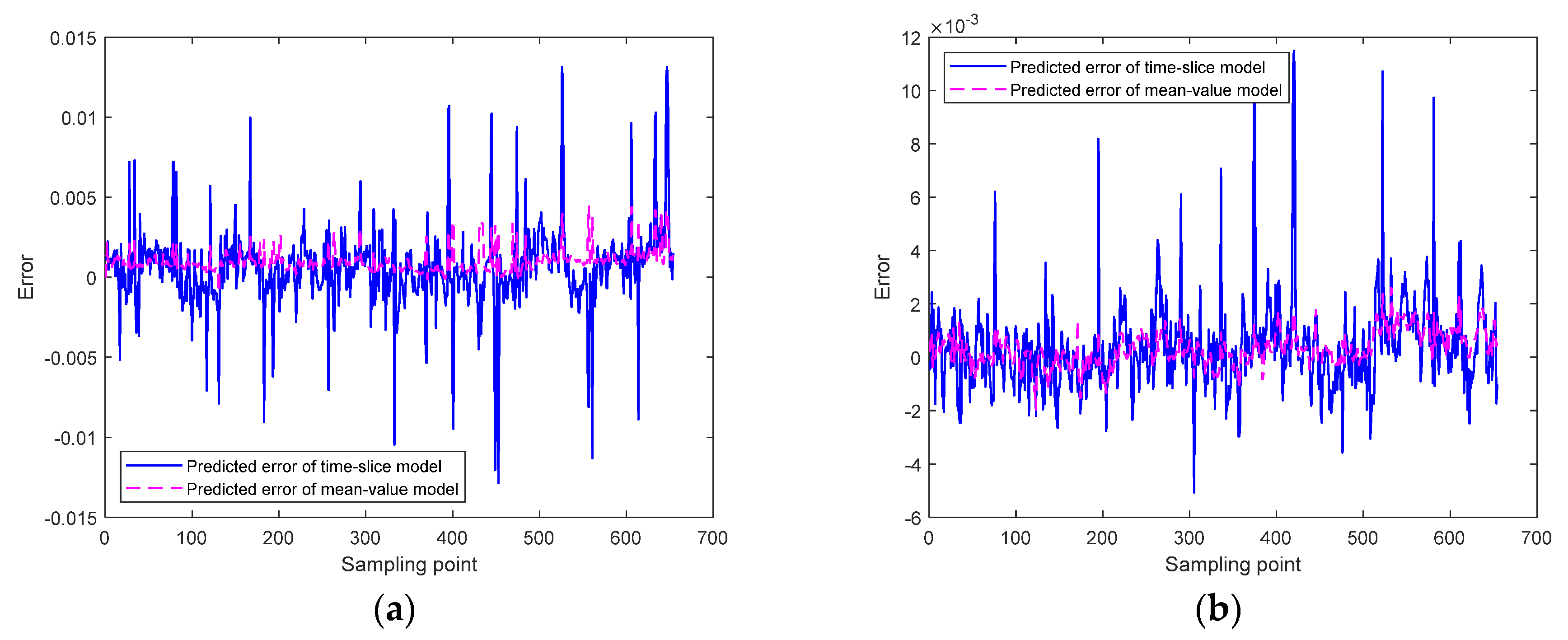Similarly, both models are used to predict the Mach number in mode 2; Figure 2b shows the predicted results. Again, the mean-value model has better prediction results than the time-slice model. The prediction errors of both models are shown in Figure 3a,b for Modes 1 and 2; the superiority of the mean-value model is clearly visible.

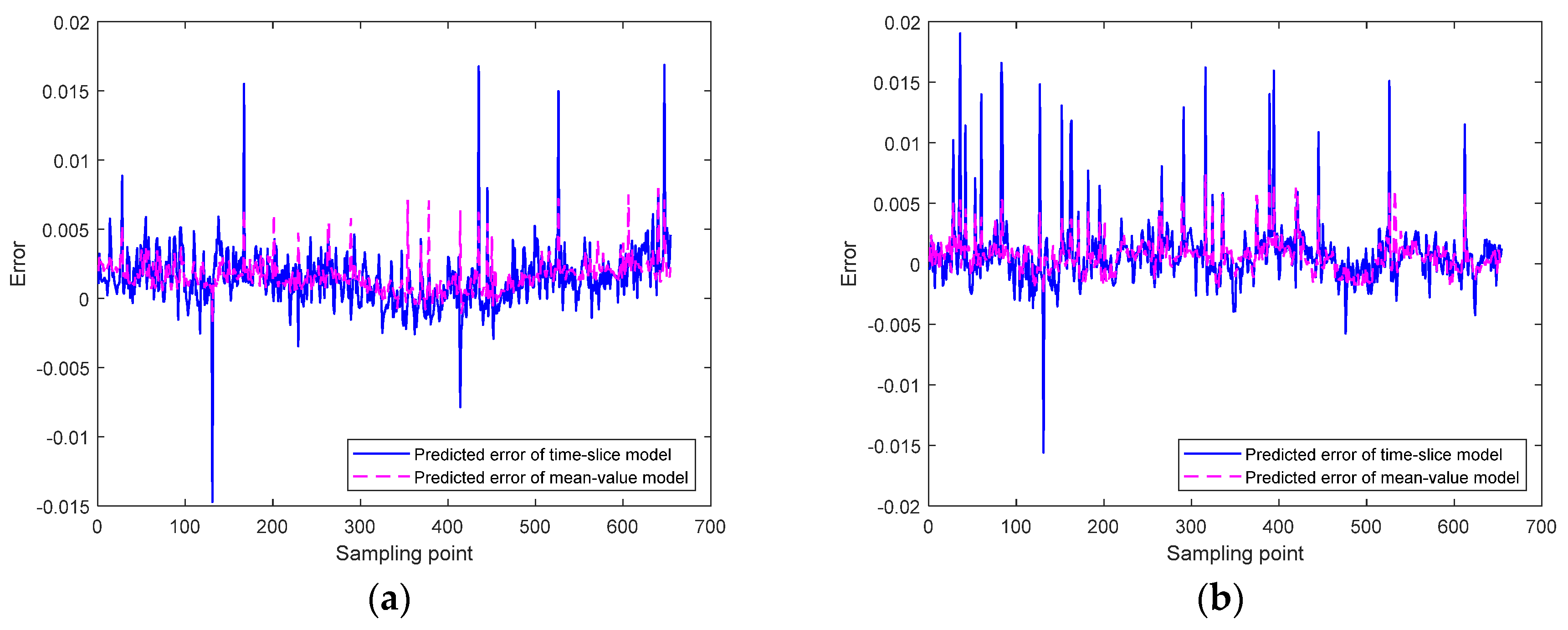
Next, Modes 1 and 2 are combined for modeling and predictions to find out whether the two modes show significant differences. Using training data 1 and 2, the regression parameters of the time-slice and mean-value models are obtained successively. Then, the Mach numbers are predicted for test data 1 and 2; the predicted results are shown in Figure 4a,b. Similarly, the mean-value model yields better prediction results than the time-slice model. The prediction errors of both models are shown in Figure 5a,b for test data 1 and 2. Once again, the superiority of the mean-value model is clearly visible.

The differences between the results in Figure 2 and Figure 4 should be clarified by the RMSE values of the predictions, which are listed in

Table 2. RMSE values obtained by using the time-slice PLS and mean-value PLS models.

Simulations	Time-Slice Model	Mean-Value Model
Test data 1 using model of mode 1	0.0023	0.0012
Test data 2 using model of mode 2	0.0012	0.0007
Test data 1 using multimode model	0.0034	0.0019
Test data 2 using multimode model	0.0020	0.0016

. By comparing the RMSE values in Table 2, it can be seen that the accuracy of the Mach number prediction obtained using the mean-value PLS model is better than that obtained using the time-slice PLS model. Further, the prediction results of the multi-mode model are worse than those of the single-mode model. In other words, during the modeling process, if the working modes are finely divided by analyzing the attack angle step or other key process variables, the prediction accuracy should improve.

3.3. Mach Predictions Based on KPLS Model

As it is known above that the mean-value model has a better effect, mean-value KPLS model will be further used for the Mach number prediction below. In order to further improve the effect of mean-value KPLS model, the original training data and some data in the test data block will be taken as a new training data set, and the mean-value KPLS model is set up, then the rest data in the test data block are used as the test data to verify the model prediction effect. Since the training data contain the information of the test data block and the test data used is a part of the test data block, the prediction model established will have better prediction effect. By the way, the predicted effect of KPLS is greatly influenced by multiple choice kernel functions. But now one can only choose the best performing kernel function by trying multiple kernels. It is still a challenge to find a systematic way of selecting the kernel function.

Firstly, the prediction results of mode 1 are obtained. Training data 1 and the first 150 sample points of test data 1 are used as the training data, and the mean-value KPLS model is established. The rest data of test data 1 are used as the test data. Figure 6a shows the predicted results of the mean-value KPLS model which are compared with those of mean-value PLS model. It can be seen that the mean-value KPLS model has better prediction results. Similarly, the prediction results of mode 2 are obtained. 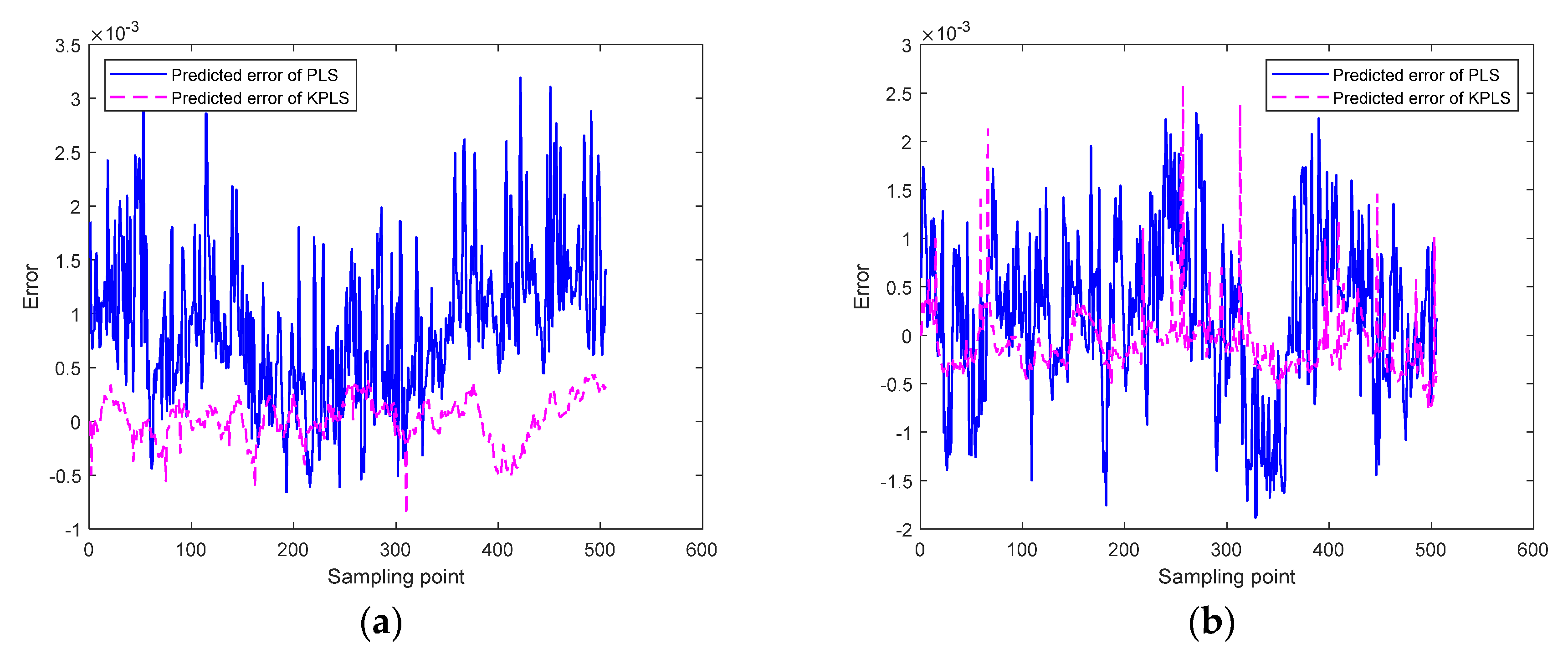And the predicted results are presented in Figure 6b. The same conclusion can be drawn that the mean-value KPLS model has better prediction results. Besides, the prediction errors of both the mean-value PLS model and the mean-value KPLS model have been shown in Figure 7a,b for mode 1 and 2, respectively, and the superiority of the mean-value KPLS model is clearly represented.

Afterwards, mode 1 and mode 2 are combined for modeling and prediction. This can test whether the two modes have so significant difference that modeling respectively is necessary. Firstly, training data 1, training data 2 and the first 150 sample points of test data 1 are used as the training data, and the mean-value KPLS model is established. The rest data of test data 1 are used as the test data. The prediction results are shown in Figure 8a and compared with those of the mean-value PLS model. Similarly, the prediction results of data block 2 are shown in Figure 8b. From Figure 8a,b, the predictions of the mean-value KPLS model are much better than those of the mean-value PLS model. Besides, the prediction errors of both the models have been shown in Figure 9a,b for test data 1 and 2, respectively, and the superiority of the mean-value KPLS model is clearly represented.

The RMSE values of the predictions are listed in

Table 3. RMSE values obtained using the mean-value PLS and mean-value KPLS models.

Simulations	Mean-Value PLS Model	Mean-Value KPLS Model
Test data 1 using model of mode 1	6.5299 × 10−4	1.8465 × 10−4
Test data 2 using model of mode 2	4.9279 × 10−4	2.5062 × 10−4
Test data 1 using multimode model	0.0011	2.0297 × 10−4
Test data 2 using multimode model	8.6771 × 10−4	3.6643× 10−4

. According to values shown in Table 3, it can be clearly seen that the mean-value KPLS model has a better prediction effect than the mean-value PLS model. It can be concluded that for a wind tunnel system with strong nonlinear characteristics, the use of the mean-value KPLS model is more appropriate than mean-value PLS modeling. Additionally, the prediction results of the multi-mode model are worse than those of the single-mode model, which is consistent with the prediction regarding the use of the time-slice PLS model and the mean-value PLS model in Section 3.2. That is, if the working modes are finely divided by analyzing key process variables, the prediction accuracy of the model will improve.

4. Conclusions

In this paper, a Mach number prediction method for wind tunnel flow fields is introduced. By applying KPLS, the nonlinear characteristics of the wind tunnel flow are well handled, and satisfactory prediction results are obtained by proper mode analysis and division. First, the time-slice PLS and mean-value PLS models are used to predict the Mach number in a multi-mode wind tunnel system. By avoiding the influence of process noises, the mean-value PLS model provides better prediction results than the time-slice PLS model in either single- or multi-mode modeling. Additionally, models for single modes show better prediction abilities than those for multiple modes, which shows the necessity of mode division according to key process variables. In order to further improve the prediction accuracy, a mean-value KPLS modeling algorithm which is suitable for nonlinear systems is adopted. Compared with the prediction effect of the PLS model, it was found that mean-value KPLS model has better prediction effect in either single or multi-mode modeling. Again, the models for single modes show better prediction abilities than those for multiple modes.

This is a trial work for Mach number predictions in a multi-mode wind tunnel flow system, which is novel and unusual in the field of wind tunnel flow control. The application of the proposed method combined with various advance control algorithms is underway, and as a result, the control accuracy of the Mach number will be improved.