
A Comparison of Three Different Group Intelligence Algorithms for Hyperspectral Imagery Classification

Abstract
:1. Introduction
2. Theoretical Methods
2.1. Feature Extraction Method
2.1.1. Principal Component Analysis (PCA)
2.1.2. Linear Discriminant Analysis (LDA)
2.1.3. Locality Preserving Projections (LPP)
2.2. Classification Methods
2.2.1. Support Vector Machine (SVM)
2.2.2. Random Forest (RF)
- (1)
- Extract k training subsets from the original training set, corresponding to k decision trees, respectively.
- (2)
- The growth of each decision tree includes two processes. First, random feature variables are selected, and n features (n ≤ N) are randomly selected at each node of each tree. The other is node splitting. The information contained in each feature is calculated, and the feature with the best classification ability is selected among n features for node splitting.
- (3)
- Generate a random forest, do not prune each tree to maximize its growth, and finally, all decision trees constitute a random forest.
- (4)
- After the random forest is constructed, the samples are input into the classifier. Each decision tree predicts the corresponding category for each sample, and records it by voting. The category with the most votes becomes the determined category of the sample.
2.2.3. K-Nearest Neighbor (KNN)
3. Data and Implementation
4. Results and Discussion
5. Conclusions
Author Contributions
Funding
Institutional Review Board Statement
Informed Consent Statement
Data Availability Statement
Acknowledgments
Conflicts of Interest
References
- Tong, Q.X.; Zhang, B.; Zhang, L.F. Advances in hyperspectral remote sensing in China. J. Remote Sens. 2016, 20, 19. [Google Scholar]
- Zhang, M.; Li, W.; Du, Q. Diverse region-based CNN for hyperspectral image classification. IEEE Trans. Image Process. 2018, 27, 2623–2634. [Google Scholar] [CrossRef] [PubMed]
- Li, P.; Wang, D.; Wang, L.; Lu, H. Deep visual tracking: Review and experimental comparison. Pattern Recognit. 2018, 76, 323–338. [Google Scholar] [CrossRef]
- Ghamisi, P.; Plaza, J.; Chen, Y.; Li, J.; Plaza, A. Advanced supervised spectral classifiers for hyperspectral images: A review. J. Latex Cl. Files 2007, 6, 1–23. [Google Scholar]
- Yang, X.; Ye, Y.; Li, X.; Lau RY, K.; Zhang, X.; Huang, X. Hyperspec-tral image classification with deep learning models. IEEE Trans. Geosci. Remote Sens. 2018, 56, 5408–5423. [Google Scholar] [CrossRef]
- Yin, X.; Wang, R.; Liu, X.; Cai, Y. Deep forest-based classification of hyperspectral images. Proc. Chin. Control Conf. 2018, 2018, 10367–10372. [Google Scholar]
- Yu, D.; Ma, Z.; Wang, R. Efficient smart grid load balancing via fog and cloud computing. Math. Probl. Eng. 2022, 22, 3151249. [Google Scholar] [CrossRef]
- Wang, X.; Feng, Y. New Method Based on Support Vector Machine in Classification for Hyperspectral Data. In Proceedings of the International Symposium on Computational Intelligence and Design, Wuhan, China, 17–18 October 2008; pp. 76–80. [Google Scholar]
- Joelsson, S.R.; Benediktsson, J.A.; Sveinsson, J.R. Random Forest Classifiers for Hyperspectral Data. In Proceedings of the 2005 IEEE International Geoscience and Remote Sensing Symposium, 2005 IGARSS ’05, Seoul, Korea, 29–29 July 2005. [Google Scholar]
- Ma, L.; Crawford, M.M.; Tian, J. Local manifold learning-based K-nearest-neighbor for hyperspectral image classification. IEEE Trans. Geosci. Remote Sens. 2010, 48, 4099–4109. [Google Scholar] [CrossRef]
- Du, P.J.; Xia, J.S.; Xue, Z.H.; Tan, K.; Su, H.J.; Bao, R. Advances in classification of hyperspectral remote sensing images. J. Remote Sens. 2016, 20, 21. [Google Scholar]
- Du, P.J.; Xia, J.S.; Zhang, W.; Tan, K.; Liu, Y.; Liu, S.C. Multiple classifier system for remote sensing image classification: A review. Sensors 2012, 12, 4764–4792. [Google Scholar] [CrossRef]
- Hughes, G.F.; Hughes, G. On the mean accuracy of statistical pattern recognizers. IEEE Trans. Inf. Theory 1968, 14, 55–63. [Google Scholar] [CrossRef] [Green Version]
- Zhang, B. Frontier of hyperspectral image processing and information extraction. J. Remote Sens. 2016, 20, 1062–1089. [Google Scholar] [CrossRef]
- Farrell, M.D.; Mersereau, R.M. On the impact of PCA dimension reduction for hyperspectral detection of difficult targets. IEEE Geosci. Remote Sens. Lett. 2005, 2, 192–195. [Google Scholar] [CrossRef]
- Tharwat, A.; Gaber, T.; Ibrahim, A.; Hassanien, A.E. Linear discriminant analysis: A detailed tutorial. AI Commun. 2017, 30, 169–190. [Google Scholar] [CrossRef] [Green Version]
- He, X.; Niyogi, P. Locality Preserving Projections. Adv. Neural Inf. Process. Syst. 2004, 16, 153–160. [Google Scholar]
- Schölkopf, B.; Smola, A.; Müller, K.R. Kernel Principal Component Analysis. In Proceedings of the 7th International Conference on Artificial Neural Networks—ICANN 1997, Lausanne, Switzerland, 8–10 October 1997; Springer-Verlag GmbH: Cham, Switzerland; pp. 583–588. [Google Scholar]
- Bach, F.R.; Jordan, M.I. Kernel independent component analysis. J. Mach. Learn. Res. 2003, 3, 1–48. [Google Scholar]
- Roweis, S.T.; Saul, L.K. Nonlinear dimensionality reduction by locally linear embedding. Science 2000, 290, 2323–2326. [Google Scholar] [CrossRef] [Green Version]
- Belkin, M.; Niyogi, P. Laplacian eigenmaps for dimensionality reduction and data representation. Neural Comput. 2003, 15, 1373–1396. [Google Scholar] [CrossRef] [Green Version]
- Bachmann, C.M.; Ainsworth, T.L.; Fusina, R.A. Exploiting manifold geometry in hyperspectral imagery. IEEE Trans. Geosci. Remote Sens. 2005, 43, 441–454. [Google Scholar] [CrossRef]
- Gepreel, K.A.; Higazy, M.; Mahdy AM, S. Optimal control, signal flow graph, and system electronic circuit realization for nonlinear Anopheles mosquito model. Int. J. Mod. Phys. C 2020, 31, 2050130. [Google Scholar] [CrossRef]
- Uddin, M.P.; Mamun, M.A.; Hossain, M.A. PCA-based feature reduction for hyperspectral remote sensing image classification. IETE Technol. Rev. 2021, 38, 377–396. [Google Scholar] [CrossRef]
- Fabiyi, S.D.; Murray, P.; Zabalza, J.; Ren, J. Folded LDA: Extending the linear discriminant analysis algorithm for feature extraction and data reduction in hyperspectral remote sensing. IEEE J. Sel. Top. Appl. Earth Obs. Remote Sens. 2021, 14, 12312–12331. [Google Scholar] [CrossRef]
- Ayesha, S.; Hanif, M.K.; Talib, R. Overview and comparative study of dimensionality reduction techniques for high dimensional data. Inf. Fusion 2020, 59, 44–58. [Google Scholar] [CrossRef]
- Su, H.J.; Gu, M.Y. Extraction of local alignment feature from hyperspectral remote sensing image based on optimization and discriminant. J. Remote Sens. 2021, 25, 16. [Google Scholar]
- Shao, W.J.; Sun, W.W.; Yang, G. Comparative analysis of texture feature extraction from hyperspectral remote sensing images. Remote Sens. Technol. Appl. 2021, 36, 10. [Google Scholar]


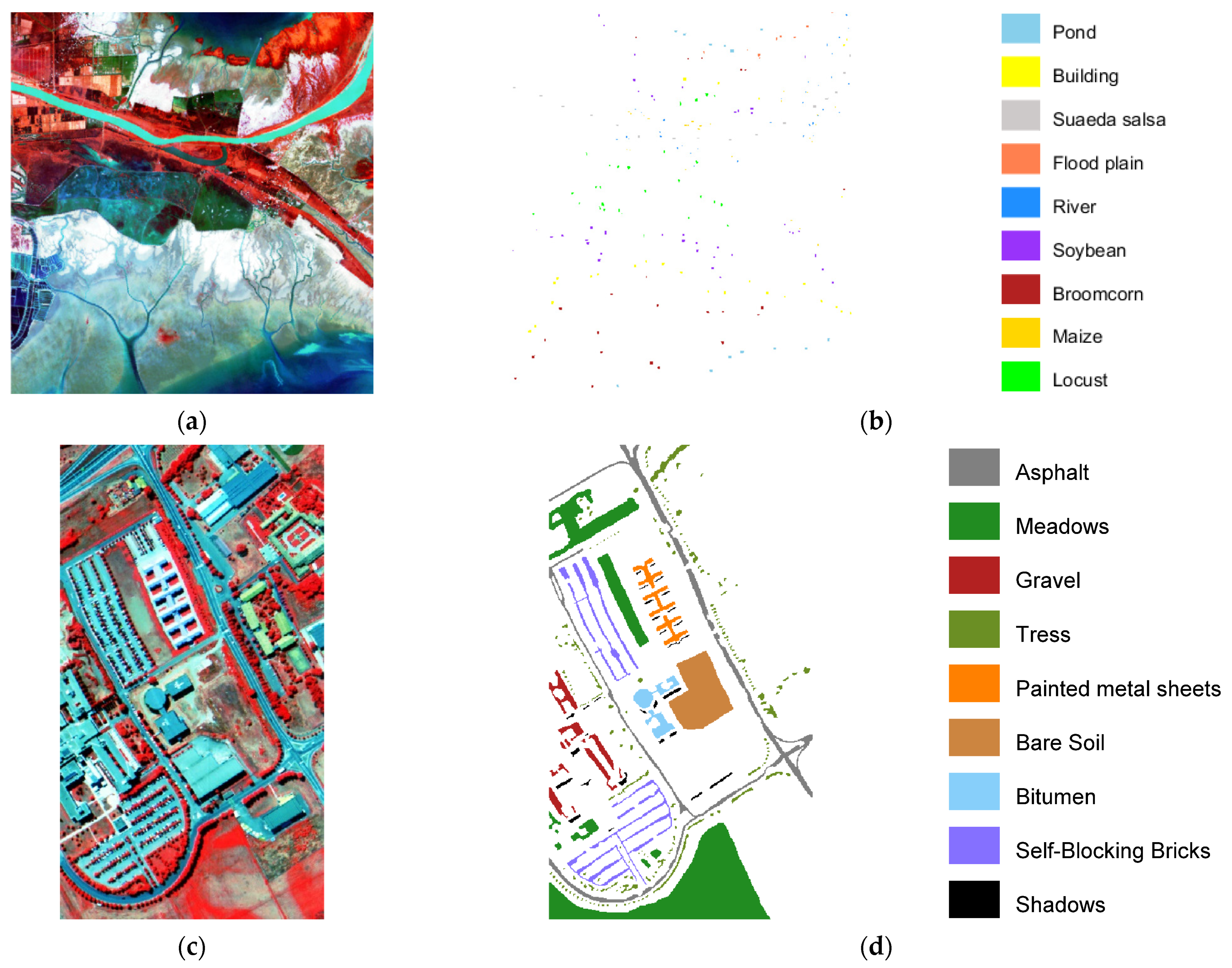
| No. | Yellow River Estuary Data | PaviaU Data | ||||
|---|---|---|---|---|---|---|
| Classes | Training Sample | Test Sample | Class | Training Sample | Test Sample | |
| 1 | Pond | 10 | 300 | Asphalt | 332 | 6299 |
| 2 | Building | 10 | 406 | Meadows | 932 | 17,717 |
| 3 | Suaeda salsa | 10 | 255 | Gravel | 105 | 1994 |
| 4 | Flood plain | 10 | 95 | Tress | 153 | 2911 |
| 5 | River | 10 | 162 | Painted metal sheets | 67 | 1278 |
| 6 | Soybean | 10 | 538 | Bare Soil | 251 | 4778 |
| 7 | Broomcorn | 10 | 369 | Bitumen | 67 | 1263 |
| 8 | Maize | 10 | 123 | Self-Blocking Bricks | 184 | 3498 |
| 9 | Locust | 10 | 367 | Shadows | 47 | 900 |
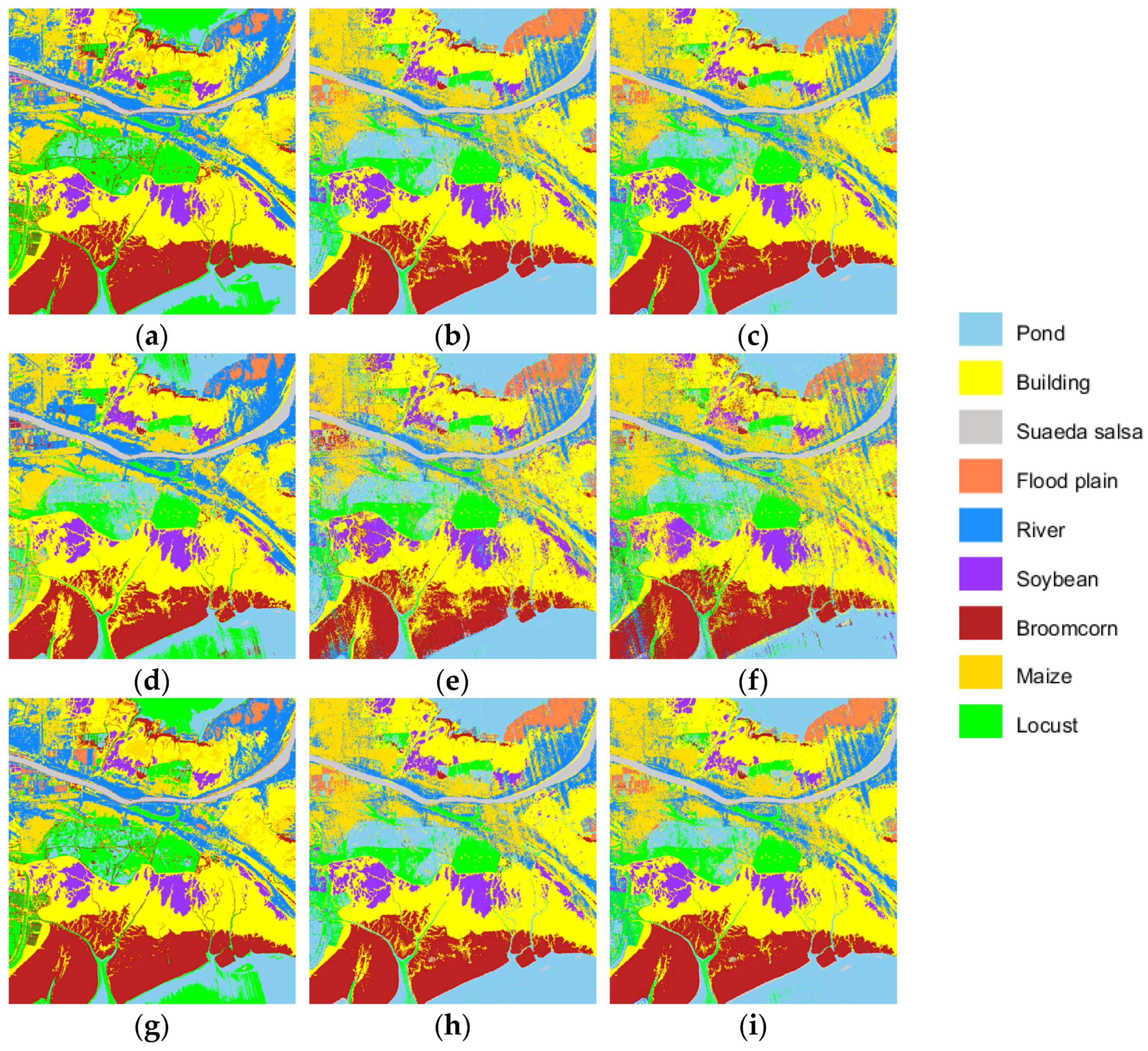
| Class Label | SVM | RF | KNN | ||||||
|---|---|---|---|---|---|---|---|---|---|
| PCA | LDA | LPP | PCA | LDA | LPP | PCA | LDA | LPP | |
| 1 | 81.67 | 99.67 | 100 | 95.67 | 100.00 | 98 | 74.33 | 99.67 | 100 |
| 2 | 100 | 100 | 100 | 100 | 97.04 | 93.6 | 99.75 | 100 | 100 |
| 3 | 100 | 100 | 100 | 100 | 98.82 | 99.61 | 100 | 100. | 100 |
| 4 | 100 | 94.74 | 93.68 | 100 | 85.26 | 85.26 | 100 | 94.74 | 93.68 |
| 5 | 95.68 | 83.33 | 81.48 | 89.51 | 66.05 | 77.16 | 92.59 | 83.33 | 81.48 |
| 6 | 100 | 98.7 | 97.4 | 99.44 | 93.68 | 88.66 | 100 | 98.7 | 97.4 |
| 7 | 99.73 | 99.19 | 98.64 | 99.46 | 96.48 | 98.37 | 100 | 99.19 | 98.64 |
| 8 | 83.74 | 95.12 | 94.31 | 91.87 | 80.49 | 95.93 | 90.24 | 95.12 | 94.31 |
| 9 | 84.74 | 74.11 | 75.2 | 76.02 | 74.66 | 71.93 | 81.2 | 74.11 | 75.2 |
| Overall classification accuracy of OA | 94.68 | 94.49 | 94.15 | 94.66 | 90.18 | 90.12 | 93.46 | 94.49 | 94.15 |
| Average classification accuracy of AA | 94.12 | 93.66 | 93.03 | 94.18 | 88.02 | 87.57 | 92.99 | 93.66 | 93.03 |
| Kappa coefficient | 93.85 | 93.63 | 93.24 | 93.83 | 88.65 | 88.61 | 92.43 | 93.63 | 93.24 |
| Class Label | SVM | RF | KNN | ||||||
|---|---|---|---|---|---|---|---|---|---|
| PCA | LDA | LPP | PCA | LDA | LPP | PCA | LDA | LPP | |
| 1 | 92.32 | 89.03 | 91.09 | 92.4 | 91.43 | 93.27 | 84.89 | 90.68 | 89.76 |
| 2 | 97.79 | 94.07 | 96 | 99.25 | 94.56 | 95.61 | 96.07 | 96.43 | 98.99 |
| 3 | 84.95 | 65.4 | 69.76 | 54.71 | 65.25 | 64.24 | 64.54 | 66.75 | 70.81 |
| 4 | 91.38 | 85.06 | 89.63 | 85.54 | 86.81 | 91.21 | 75.27 | 82.79 | 86.98 |
| 5 | 99.3 | 99.77 | 99.77 | 99.53 | 99.77 | 100 | 98.83 | 99.61 | 99.61 |
| 6 | 88.45 | 73.44 | 76.33 | 45.25 | 76.39 | 80.98 | 53.39 | 71.45 | 72.67 |
| 7 | 86.46 | 42.36 | 63.34 | 53.13 | 42.28 | 63.90 | 80.52 | 62.87 | 81.08 |
| 8 | 89.57 | 76.96 | 83.73 | 92.11 | 77.04 | 82.59 | 81.16 | 78.24 | 84.16 |
| 9 | 99.89 | 99.44 | 99.67 | 99.89 | 98.56 | 99.11 | 99.89 | 99 | 98.89 |
| Overall classification accuracy of OA | 93.79 | 86.03 | 89.31 | 86.62 | 87.13 | 89.82 | 84.69 | 87.72 | 90.41 |
| Average classification accuracy of AA | 92.84 | 83.94 | 88.18 | 91.18 | 86.13 | 89.24 | 84.94 | 87.02 | 89.88 |
| Kappa coefficient | 91.74 | 81.34 | 85.72 | 81.64 | 82.82 | 86.46 | 79.22 | 83.49 | 87.1 |
| Dataset | SVM | RF | KNN | ||||||
|---|---|---|---|---|---|---|---|---|---|
| PCA | LDA | LPP | PCA | LDA | LPP | PCA | LDA | LPP | |
| Yellow River Estuary | 0.08 | 0.03 | 0.01 | 3.13 | 1.65 | 2.73 | 0.06 | 0.01 | 0.01 |
| University of Pavia | 2.15 | 0.85 | 1.26 | 29.23 | 11.36 | 18.41 | 0.48 | 0.03 | 0.3 |
Publisher’s Note: MDPI stays neutral with regard to jurisdictional claims in published maps and institutional affiliations. |
© 2022 by the authors. Licensee MDPI, Basel, Switzerland. This article is an open access article distributed under the terms and conditions of the Creative Commons Attribution (CC BY) license (https://creativecommons.org/licenses/by/4.0/).
Share and Cite
Wang, Y.; Zeng, W. A Comparison of Three Different Group Intelligence Algorithms for Hyperspectral Imagery Classification. Processes 2022, 10, 1672. https://doi.org/10.3390/pr10091672
Wang Y, Zeng W. A Comparison of Three Different Group Intelligence Algorithms for Hyperspectral Imagery Classification. Processes. 2022; 10(9):1672. https://doi.org/10.3390/pr10091672
Chicago/Turabian StyleWang, Yong, and Weibo Zeng. 2022. "A Comparison of Three Different Group Intelligence Algorithms for Hyperspectral Imagery Classification" Processes 10, no. 9: 1672. https://doi.org/10.3390/pr10091672