State Feedback Stabilization for a Class of Upper-Triangular Stochastic Nonlinear Systems with Time-Varying Control Coefficients

Abstract

The problem explored in this article concerns the stability of the state feedback control of the upper-triangular stochastic nonlinear systems whose control coefficients are time-varying. First, the state feedback control of the corresponding nominal system is carried out by utilizing the backstepping technique combined with the appropriate Lyapunov function. Then, low-gain homogeneous domination technology and the efficient coordinate transformation method are adopted to realize the state feedback control of the original system and ensure the global asymptotic stability (GAS) in probability of the system. Finally, an example is given to illustrate the feasibility and correctness of the method.

1. Introduction

The stability of stochastic systems occupies an essential place in the field of nonlinear control. On the one hand, it has an important theoretical value [1,2,3,4,5,6,7,8,9]. On the other hand, it has a strong practical significance [10,11,12]. It is worth noting that many physical systems such as dynamic ship positioning systems [10], robotic manipulators on seaborne platforms [11], and wireless sensor networks [12] can all be described by stochastic systems. In the past few years, many research works have been published on stochastic nonlinear systems [13,14,15,16,17,18,19,20,21,22,23], in which a quadratic or a quartic Lyapunov function is usually designed to tackle the stability problem of stochastic nonlinear systems.

Stochastic systems are commonly divided into two types, namely upper-triangular (i.e., feedforward) stochastic systems and lower-triangular (i.e., feedback) stochastic systems. In recent years, the control issues of lower-triangular stochastic nonlinear systems have become the focus of prominent research works with the assistance of the stochastic stability theory [24,25,26,27,28,29,30,31]. Among them, Refs. [29,30,31] are able to solve the stability problem of lower-triangular stochastic nonlinear systems through a homogeneous domination technology. The upper-triangle stochastic nonlinear systems have also attracted extensive attention due to its wide application in machinery and the aerospace industry. For example, the cart–pendulum system [32] and the vertical take-off and landing aircraft [33] can all be modeled as the upper-triangular structure. However, due to the particularity and complexity of the structure of the upper-triangular stochastic systems, many traditional methods such as the backstepping method are no longer applicable. This is because in the differential transformation of the Lyapunov function, stochastic differentiation produces a Hessian cross term for the diffusion term of the system, which makes the stability of the upper-triangular stochastic systems very challenging.

For upper-triangular systems, Ref. [34] introduces a scale gain into the controller to control the disturbance by using the homogeneous domination technology and generalizes this result to the upper-triangular stochastic nonlinear systems. Ref. [35] proposes a method for tackling the stability problem on the basis of the homogeneous domination technique, i.e., the low-gain homogeneous domination technique. Ref. [36] then studies the stability problem of an upper-triangular stochastic system by utilizing the method for the first time. Furthermore, the stability problems of large-scale [37] and high-order [38] upper-triangular stochastic nonlinear systems as well as those disturbed by a second-order moment [39] are investigated by utilizing the low-gain homogeneous domination technique. However, we can notice that the systems in [36,37,38,39] are all with deterministic control coefficients. Compared with deterministic control coefficients, time-varying control coefficients have also received extensive attention [40], where only stochastic linear systems have been studied. The stability problem of upper-triangular stochastic nonlinear systems with time-varying control coefficients has not been researched.

On the basis of the above-mentioned literature, this paper utilizes the Lyapunov function and low-gain homogeneous domination technique to analyze the stability of the state feedback of the upper-triangular stochastic systems, which have time-varying control coefficients. This study includes at least two important contributions:

(i) The structure of the upper-triangular systems is complex. Therefore, in this article, a stability analysis of the nominal system is firstly carried out, and then the state feedback stability problem of the studied systems is solved by utilizing the low-gain homogeneous domination technique.

(ii) This paper considers general upper-triangular stochastic systems. This is in contrast to [36,37,38,39], which consider that the control coefficients of the systems are deterministic, while we study the systems with time-varying control coefficients. Time-varying control coefficients have uncertain upper and lower bounds, which, together with Young’s inequality, ensure that the stability problem is solved.

The remaining parts are as follows. Section 2 presents relevant definitions. Section 3 discusses the main results. A numerical simulation is presented in Section 4. Finally, Section 5 brings the paper to a conclusion.

2. Relevant Definitions

The following symbols are commonly used in this paper. $R_{+}$ means the set of all nonnegative real numbers, and $R^n$ means the real n-dimensional space. $X^T$ is its transpose, $\mathrm{Tr}\left\{X\right\}$ is recorded as its trace when X is square, and $\left|X\right|$ indicates the 2-norm of vector X in Euclidean space. For $A=A_{ij}\in R^{n\times m}$, defining $\left|A\right|={\left({\sum }_{i=1}^n{\sum }_{j=1}^m{A}_{ij}^2\right)}^{1/2}$ and ${\left|A\right|}_{\infty }={max}_{1\le i\le n}\{{\sum }_{j=1}^m|A_{ij}\left|\right\}$. ${\mathcal{C}}^i$ is recorded as the set of all functions with a continuous ith partial derivative. Class $\mathcal{K}$ indicates all of the $R_{+}\to R_{+}$ functions that are continuous, strictly monotonic, and equal to zero at zero; class ${\mathcal{K}}_{\infty }$ indicates all the unbounded functions in $\mathcal{K}$; the function $\beta (s,t)\in \mathcal{KL}$: $R_{+}\times R_{+}\to R_{+}$ indicates that for a given t, $\beta (s,t)\in \mathcal{K}$, while for a given s, $\beta (s,t)$ is monotonically decreasing, and ${lim}_{t\to \infty }\beta (s,t)=0$.

For the stochastic nonlinear system

$$\begin{array}{c}\hfill dx=f\left(x\right)dt+g^T\left(x\right)d\omega ,\forall x_0\in R^n,\end{array}$$

(1)

where the state is $x\in R^n$, $\omega \in R^r$ is a Wiener process for independent standards defined in a probability space $(\mathrm{\Omega },\mathcal{F},P)$. For any $t\ge 0$, when $x\in R^n$, the functions $f:R^n\to R^n$, $g^T:R^n\to R^{n\times r}$ are locally Lipschitz, and $f\left(0\right)=0$, $g\left(0\right)=0$. The following definitions are available.

Definition 1

([22]). $\forall \epsilon >0$, $\exists \beta (·,·)\in \mathcal{KL}$, satisfying $P\left\{\left|x\left(t\right)\right|<\beta \left(\right|x_0|,t)\right\}\ge 1-\epsilon$, for $\forall t\ge 0$, $x_0\in R^n\setminus \left\{0\right\}$, then system (1) is said to be globally asymptotically stable in probability, with an equilibrium point of $x=0$.

Definition 2

([35]). For the coordinates $(x_1,\cdots ,$$x_n)\in R^n$ and $0<r_i\in R$, $i=1,\cdots ,n$:

(1) $\forall \epsilon >0$, defining the dilation ${△}_{\epsilon }\left(x\right)=({\epsilon }^{r_1}{x}_1,\cdots ,$${\epsilon }^{r_n}{x}_n)$, where $r_i$ is the weight of the corresponding coordinates. For convenience, we define $△=(r_1,\cdots ,r_n)$;

(2) If $\tau \in R$, for $\forall x\in R^n\setminus \left\{0\right\}$, $\epsilon >0$, $V\left({△}_{\epsilon }\left(x\right)\right)={\epsilon }^{\tau }V(x_1,\cdots ,x_n)$, then the scalar function $V\in \mathcal{C}(R^n,R)$ and the vector function $f\in \mathcal{C}(R^n,R)$ are homogeneous of degree τ;

(3) For $\forall x\in R^n$, such that ${\parallel x\parallel }_{△}=({\sum }_{i=1}^n|x_i{{|}^{2/r_i})}^{1/2}$.

3. Main Results

Consider the following upper-triangular stochastic nonlinear systems in this paper:

$$\begin{array}{cc}\hfill d{x}_1& =\left(d_1\left(t\right)x_2+f_1\left({\tilde{x}}_3\right)\right)dt+g_1^T\left({\tilde{x}}_3\right)d\omega ,\hfill \\ \hfill d{x}_2& =\left(d_2\left(t\right)x_3+f_2\left({\tilde{x}}_4\right)\right)dt+g_2^T\left({\tilde{x}}_4\right)d\omega ,\hfill \\ \hfill & ⋮\hfill \\ \hfill d{x}_{n-2}& =\left(d_{n-2}\left(t\right)x_{n-1}+f_{n-2}\left({\tilde{x}}_n\right)\right)dt+g_{n-2}^T\left({\tilde{x}}_n\right)d\omega ,\hfill \\ \hfill d{x}_{n-1}& =d_{n-1}\left(t\right)x_{n}dt,\hfill \\ \hfill d{x}_n& =d_n\left(t\right)udt,\hfill \end{array}$$

(2)

where $x={(x_1,\cdots ,x_n)}^T\in R^n$ and $u\in R$ are respectively the system state and the input, while ${\tilde{x}}_i={(x_i,\cdots ,x_n)}^T\in R^n$, $\omega \in R^r$ is a Wiener process for independent standards defined in a probability space $(\mathrm{\Omega },\mathcal{F},P)$. For $i=1,\cdots ,n-2$, the functions $f_i:R^{n-i-1}\to R$ and $g_i:R^{n-i-1}\to R^r$ both vanish at the origin, and for $i=1,\cdots ,n$, $d_i\left(t\right):R_{+}\to R$ are unknown time-varying control coefficients with a known sign.

To study system (2), we make the following assumptions:

Assumption 1.

There is a constant $b>0$ for $i=1,\cdots ,n$, such that the following equation holds:

$$\begin{array}{cc}\hfill |f_i\left({\tilde{x}}_{i+2}\right)|& \le b\left(\right|x_{i+2}|+\cdots +|x_n\left|\right),\hfill \\ \hfill |g_i\left({\tilde{x}}_{i+2}\right)|& \le b\left(\right|x_{i+2}|+\cdots +|x_n\left|\right).\hfill \end{array}$$

(3)

Assumption 2.

Suppose that the symbol for $d_i\left(t\right),t\in R_{+}$ is positive, and for $i=1,\cdots ,n$, there are unknown normal numbers ${\lambda }_i$, ${\mu }_i$, and μ, such that

$$\begin{array}{c}\hfill 0<{\lambda }_i\le d_i\left(t\right)\le {\mu }_i\le \mu .\end{array}$$

(4)

Remark 1.

According to Assumption 1, the nonlinear terms $f_i\left({\tilde{x}}_{i+2}\right)$ and $g_i\left({\tilde{x}}_{i+2}\right)$ of system (2) depend on $x_{i+2},\cdots ,x_n$, which results the upper-triangular structure. As discussed in deterministic upper-triangular systems [35,41,42] and stochastic upper-triangular systems [36,37,43,44], Assumption 1 is a reasonable assumption. Assumption 2 shows that $d_i\left(t\right)$ is time-varying, and that both upper and lower bounds are unknown, which is more general than systems [36,37,38,39] with deterministic control coefficients.

3.1. State Feedback Control of Nominal Systems

We first consider the state feedback control of nominal systems:

$$\begin{array}{cc}\hfill d{z}_i& =d_i\left(t\right)z_{i+1}dt,i=1,\cdots ,n-1,\hfill \\ \hfill d{z}_n& =d_n\left(t\right)vdt.\hfill \end{array}$$

(5)

Next, we design an appropriate state feedback controller using the backstepping method and then conduct a stability analysis.

Step 1. Choosing a coordinate change ${\xi }_1=z_1$ and the Lyapunov function $V_1\left({\overline{z}}_1\right)=\frac{1}{4}{\xi }_1^4$ from (5), it follows that

$$\begin{array}{cc}\hfill \mathcal{L}{V}_1\left({\overline{z}}_1\right)& \le \frac{\partial V_1}{\partial z_1}{d}_1{z}_2\le d_1{z}_1^3(z_2-z_2^{*})+d_1{z}_1^3{z}_2^{*}.\hfill \end{array}$$

(6)

With Assumption 2, we have

$$\begin{array}{c}\hfill d_1{z}_1^3{z}_2^{*}\le \mu z_1^3{z}_2^{*}.\end{array}$$

(7)

Then, by adding the term $\mu c_1{\xi }_1^4$ to the right side of Equation (6) and then subtracting it, and by utilizing (7), we get

$$\begin{array}{c}\hfill \mathcal{L}{V}_1\left({\overline{z}}_1\right)\le -\mu c_1{\xi }_1^4+\mu c_1{\xi }_1^4+d_1{\xi }_1^3(z_2-z_2^{*})+\mu {\xi }_1^3{z}_2^{*},\end{array}$$

(8)

where $c_1>0$ is a design parameter.

Clearly, selecting the virtual controller

$$\begin{array}{cc}\hfill z_2^{*}& =-c_1{\xi }_1:=-{\alpha }_1{\xi }_1\hfill \end{array}$$

(9)

results in

$$\begin{array}{c}\hfill \mathcal{L}{V}_1\left({\overline{z}}_1\right)\le -\mu c_1{\xi }_1^4+d_1{\xi }_1^3(z_2-z_2^{*}).\end{array}$$

(10)

Step 2. In choosing ${\xi }_2=z_2-z_2^{*}$ and the Lyapunov function $V_2\left({\overline{z}}_2\right)=V_1\left({\overline{z}}_1\right)+\frac{1}{4}{\xi }_2^4$, we can easily derive

$$\begin{array}{c}\hfill \mathcal{L}{V}_2\left({\overline{z}}_2\right)\le -\mu c_1{\xi }_1^4+d_1{\xi }_1^3{\xi }_2+d_2{\xi }_2^3(z_3-z_3^{*})+d_2{\xi }_2^3{z}_3^{*}-d_1{\xi }_2^3\frac{\partial z_2^{*}}{\partial z_1}{z}_2.\end{array}$$

(11)

By Lemma A4 (Appendix A) and Assumption 2, we have

$$\begin{array}{c}\hfill d_1{\xi }_1^3{\xi }_2\le \mu \frac{3}{4}{\epsilon }_{211}{\xi }_1^4+\mu \frac{1}{4}{\epsilon }_{211}^{-3}{\xi }_2^4,\end{array}$$

(12)

and

$$\begin{array}{cc}\hfill -d_1{\xi }_2^3\frac{\partial z_2^{*}}{\partial z_1}{z}_2& =-d_1{\xi }_2^3\frac{\partial z_2^{*}}{\partial z_1}({\xi }_2-{\alpha }_1{\xi }_1)\hfill \\ \hfill & \le \mu \left|\frac{\partial z_2^{*}}{\partial z_1}\right|{\xi }_2^4+\mu \left|\frac{\partial z_2^{*}}{\partial z_1}\right|{\left|{\xi }_2\right|}^3\left|{\xi }_1\right|{\alpha }_1\hfill \\ \hfill & \le \mu \frac{1}{4}{\overline{\epsilon }}_{212}{\xi }_1^4+\mu \sqrt{1+{\left(\frac{\partial z_2^{*}}{\partial z_1}\right)}^2}{\xi }_2^4+\mu \frac{3}{4}{\overline{\epsilon }}_{212}^{-\frac{1}{3}}{\left({\alpha }_1\sqrt{1+{\left(\frac{\partial z_2^{*}}{\partial z_1}\right)}^2}\right)}^{\frac{4}{3}}{\xi }_2^4,\hfill \end{array}$$

(13)

where ${\epsilon }_{211}>0$ and ${\overline{\epsilon }}_{212}>0$ are design parameters.

According to (12) and (13), normal numbers $c_{21}$ and $H_{21}$ are defined as

$$\begin{array}{cc}\hfill c_{21}& =\frac{3}{4}{\epsilon }_{211}+\frac{1}{4}{\overline{\epsilon }}_{212},\hfill \\ \hfill H_{21}& =\frac{1}{4}{\epsilon }_{211}^{-3}+\sqrt{1+{\left(\frac{\partial z_2^{*}}{\partial z_1}\right)}^2}+\frac{3}{4}{\overline{\epsilon }}_{212}^{-\frac{1}{3}}{\left({\alpha }_1\sqrt{1+{\left(\frac{\partial z_2^{*}}{\partial z_1}\right)}^2}\right)}^{\frac{4}{3}}.\hfill \end{array}$$

(14)

Based on Assumption 2, we have

$$\begin{array}{c}\hfill d_2{z}_2^3{z}_3^{*}\le \mu z_2^3{z}_3^{*}.\end{array}$$

(15)

Therefore, substituting (12)–(15) into (11) results in

$$\begin{array}{c}\hfill \mathcal{L}{V}_2\left({\overline{z}}_2\right)\le -\mu c_1{\xi }_1^4+d_2{\xi }_2^3(z_3-z_3^{*})+d_2{\xi }_2^3{z}_3^{*}+\mu c_{21}{\xi }_1^4+\mu H_{21}{\xi }_2^4.\end{array}$$

(16)

Adding the term $\mu c_2{\xi }_2^4$ to the right side of Equation (16) and then subtracting it results in

$$\begin{array}{cc}\hfill \mathcal{L}{V}_2\left({\overline{z}}_2\right)& \le d_2{\xi }_2^3(z_3-z_3^{*})+\mu {\xi }_2^3{z}_3^{*}-\mu (c_1-c_{21}){\xi }_1^4+\mu (c_2+H_{21}){\xi }_2^4-\mu c_2{\xi }_2^4,\hfill \end{array}$$

(17)

where $c_2>0$ is the selected design parameter, and $c_1-c_{21}>0$ by choosing the appropriate design parameters.

The smooth virtual control $z_3^{*}$ is shown below:

$$\begin{array}{c}\hfill z_3^{*}=-(c_2+H_{21}){\xi }_2:=-{\alpha }_2{\xi }_2,\end{array}$$

(18)

and by substituting (18) into (17), we have

$$\begin{array}{cc}\hfill \mathcal{L}{V}_2\left({\overline{z}}_2\right)& \le d_2{\xi }_2^3(z_3-z_3^{*})-\mu (c_1-c_{21}){\xi }_1^4-\mu c_2{\xi }_2^4.\hfill \end{array}$$

(19)

Step i. Suppose that at step $i-1$, there exists a positive definite and ${\mathcal{C}}^2$ Lyapunov function $V_{i-1}\left({\overline{z}}_{i-1}\right)$ as well as a set of definitions for the following virtual controllers $z_2^{*},\cdots ,z_i^{*}$

$$\begin{array}{cc}\hfill z_2^{*}& =-{\alpha }_1{\xi }_1,\hfill \\ \hfill & ⋮\hfill & \hfill \\ \hfill z_i^{*}& =-{\alpha }_{i-1}{\xi }_{i-1},\hfill \end{array}$$

(20)

where ${\xi }_j=z_j-z_j^{*}(1\le j\le i-1)$ and ${\alpha }_k(1\le k\le i-1)$ are normal numbers; thus,

$$\begin{array}{cc}\hfill \mathcal{L}{V}_{i-1}\left({\overline{z}}_{i-1}\right)& \le -\mu \sum _{j=1}^{i-1}\left(c_j-\sum _{k=j+1}^{i-1}{c}_{kj}\right){\xi }_j^4+d_{i-1}{\xi }_{i-1}^3(z_i-z_i^{*}),\hfill \end{array}$$

(21)

where $c_j-{\sum }_{k=j+1}^{i-1}{c}_{kj}>0$ by choosing the appropriate design parameters.

To continue with the induction, we can select ${\xi }_i=z_i-z_i^{*}$ and the following Lyapunov function in the ith step:

$$\begin{array}{cc}\hfill & V_i\left({\overline{z}}_i\right)=V_{i-1}\left({\overline{z}}_{i-1}\right)+\frac{1}{4}{\xi }_i^4,\hfill \end{array}$$

(22)

where ${\overline{z}}_i={(z_1,\cdots ,z_i)}^T$. From (21) and (22), we get

$$\begin{array}{cc}\hfill \mathcal{L}{V}_i\left({\overline{z}}_i\right)& \le -\mu \sum _{j=1}^{i-1}\left(c_j-\sum _{k=j+1}^{i-1}{c}_{kj}\right){\xi }_j^4+d_{i-1}{\xi }_{i-1}^3{\xi }_i\hfill \\ \hfill & +d_i{\xi }_i^3(z_{i+1}-z_{i+1}^{*})+d_i{\xi }_i^3{z}_{i+1}^{*}-{\xi }_i^3\sum _{k=1}^{i-1}\frac{\partial z_{i+1}}{\partial z_k}{d}_k{z}_{k+1}.\hfill \end{array}$$

(23)

From (20), Assumption 2, and Lemma A4 (Appendix A), we can conclude that

$$\begin{array}{cc}\hfill d_{i-1}{\xi }_{i-1}^3\xi i& \le \mu \frac{3}{4}{\epsilon }_{i,i-1,1}{\xi }_{i-1}^4+\mu \frac{1}{4}{\epsilon }_{i,i-1,1}^{-3}{\xi }_i^4,\hfill \\ \hfill -{\xi }_i^3\sum _{k=1}^{i-1}\frac{\partial z_i^{*}}{\partial z_k}{d}_k{z}_{k+1}& \le \mu {\left|{\xi }_i\right|}^3\sum _{k=1}^{i-2}\left|\frac{\partial z_i^{*}}{\partial z_k}\right|\left|{\xi }_{k+1}\right|+\mu {\left|{\xi }_i\right|}^3\sum _{k=1}^{i-2}\left|\frac{\partial z_i^{*}}{\partial z_k}\right|\left|{\alpha }_k{\xi }_k\right|\hfill \\ \hfill & +\mu \left|\frac{\partial z_i^{*}}{\partial z_{i-1}}\right|{\left|{\xi }_i\right|}^4+\mu {\left|{\xi }_i\right|}^3\left|\frac{\partial z_i^{*}}{\partial z_{i-1}}\right|\left|{\alpha }_{i-1}{\xi }_{i-1}\right|\hfill \\ \hfill & \le \mu \sum _{k=2}^{i-2}\frac{1}{4}{\epsilon }_{ik2}{\xi }_k^4+\mu \sum _{k=1}^{i-2}\frac{3}{4}{\epsilon }_{i,k+1,2}^{-\frac{1}{3}}{\left(\sqrt{1+{\left(\frac{\partial z_i^{*}}{\partial z_k}\right)}^2}\right)}^{\frac{4}{3}}{\xi }_i^4\hfill \\ \hfill & +\mu \sum _{k=1}^{i-2}\frac{1}{4}{\overline{\epsilon }}_{ik2}{\xi }_k^4+\mu \sum _{k=1}^{i-2}\frac{3}{4}{\overline{\epsilon }}_{ik2}^{-\frac{1}{3}}{\left({\alpha }_k\sqrt{1+{\left(\frac{\partial z_i^{*}}{\partial z_k}\right)}^2}\right)}^{\frac{4}{3}}{\xi }_i^4\hfill \\ \hfill & +\mu \sqrt{1+{\left(\frac{\partial z_i^{*}}{\partial z_{i-1}}\right)}^2}{\xi }_i^4+\mu \frac{1}{4}{\overline{\epsilon }}_{i,i-1,2}{\xi }_{i-1}^4\hfill \\ \hfill & +\mu \frac{3}{4}{\overline{\epsilon }}_{i,i-1,2}^{-\frac{1}{3}}{\left({\alpha }_{i-1}\sqrt{1+{\left(\frac{\partial z_i^{*}}{\partial z_{i-1}}\right)}^2}\right)}^{\frac{4}{3}}{\xi }_i^4.\hfill \end{array}$$

(24)

By (24), the normal numbers $c_{ik}$ and $H_{i1}$ can be defined as follows:

$$\begin{array}{cc}\hfill c_{i1}& =\frac{1}{4}{\overline{\epsilon }}_{i12},\hfill \\ \hfill c_{ik}& =\frac{1}{4}{\overline{\epsilon }}_{ik2}+\frac{1}{4}{\epsilon }_{ik2},k=2,\cdots ,i-2,\hfill \\ \hfill c_{i,i-1}& =\frac{3}{4}{\epsilon }_{i,i-1,1}+\frac{1}{4}{\epsilon }_{i,i-1,2}+\frac{1}{4}{\overline{\epsilon }}_{i,i-1,2},\hfill \\ \hfill H_{i1}& =\frac{1}{4}{\epsilon }_{i,i-1,1}^{-3}+\sum _{k=1}^{i-2}\frac{3}{4}{\epsilon }_{i,k+1,2}^{-\frac{1}{3}}{\left(\sqrt{1+{\left(\frac{\partial z_i^{*}}{\partial z_k}\right)}^2}\right)}^{\frac{4}{3}}\hfill \\ \hfill & +\sum _{k=1}^{i-2}\frac{3}{4}{\overline{\epsilon }}_{ik2}^{-\frac{1}{3}}{\left({\alpha }_k\sqrt{1+{\left(\frac{\partial z_i^{*}}{\partial z_k}\right)}^2}\right)}^{\frac{4}{3}}+\sqrt{1+{\left(\frac{\partial z_i^{*}}{\partial z_{i-1}}\right)}^2}\hfill \\ \hfill & +\frac{3}{4}{\overline{\epsilon }}_{i,i-1,2}^{-\frac{1}{3}}{\left({\alpha }_{i-1}\sqrt{1+{\left(\frac{\partial z_i^{*}}{\partial z_{i-1}}\right)}^2}\right)}^{\frac{4}{3}},\hfill \end{array}$$

(25)

where ${\epsilon }_{i,i-1,j}(j=1,2)$ and ${\epsilon }_{ik2}(k=1,\cdots ,i-1)$ are normal numbers.

By adding and subtracting $\mu c_i{\xi }_i^4$ on the right side of (23) and then using (24) and (25) in (23) results in

$$\begin{array}{cc}\hfill \mathcal{L}{V}_i\left({\overline{z}}_i\right)& \le -\mu \sum _{j=1}^{i-1}\left(c_j-\sum _{k=j+1}^{i-1}{c}_{kj}\right){\xi }_j^4+d_i{\xi }_i^3(z_{i+1}-z_{i+1}^{*})+d_i{\xi }_i^3{z}_{i+1}^{*}\hfill \\ \hfill & +\mu \sum _{k=1}^{i-1}{c}_{ik}{\xi }_k^4+\mu H_{i1}{\xi }_i^4+\mu c_i{\xi }_i^4-\mu c_i{\xi }_i^4.\hfill \end{array}$$

(26)

Clearly, by choosing the virtual controller as

$$\begin{array}{c}\hfill z_{i+1}^{*}=-(c_i+H_{i1}){\xi }_i:=-{\alpha }_i{\xi }_i,\end{array}$$

(27)

we get

$$\begin{array}{c}\hfill \mathcal{L}{V}_i\left({\overline{z}}_i\right)\le -\mu \sum _{j=1}^i\left(c_j-\sum _{k=j+1}^i{c}_{kj}\right){\xi }_j^4+d_i{\xi }_i^3(z_{i+1}-z_i^{*}),\end{array}$$

(28)

where $c_j-{\sum }_{k=j+1}^i{c}_{kj}>0$ by choosing the appropriate design parameters.

Step n. Consider the Lyapunov function for system (5):

$$\begin{array}{c}\hfill V_n\left({\overline{z}}_n\right)=V_{n-1}\left({\overline{z}}_{n-1}\right)+\frac{1}{4}{\xi }_n^4,\end{array}$$

(29)

where ${\xi }_n=z_n-z_n^{*}$. By (23), we have

$$\begin{array}{cc}\hfill \mathcal{L}{V}_n\left({\overline{z}}_n\right)& \le -\mu \sum _{j=1}^{n-1}\left(c_j-\sum _{k=j+1}^{n-1}{c}_{kj}\right){\xi }_j^4+d_n{\xi }_n^{3}v\hfill \\ \hfill & +\mu \sum _{k=1}^{n-1}{c}_{nk}{\xi }_k^4+\mu H_{n1}{\xi }_n^4+\mu c_n{\xi }_n^4-\mu c_n{\xi }_n^4,\hfill \end{array}$$

(30)

where $c_j-{\sum }_{k=j+1}^{n-1}{c}_{kj}>0$ by choosing the appropriate design parameters. Obviously, designing the state feedback control law

$$\begin{array}{c}\hfill v=-(c_n+H_{n1}){\xi }_n:=-{\alpha }_n{\xi }_n\end{array}$$

(31)

yields

$$\begin{array}{c}\hfill \mathcal{L}{V}_n\left({\overline{z}}_n\right)\le -\mu \sum _{j=1}^n\left(c_j-\sum _{k=j+1}^n{c}_{kj}\right){\xi }_j^4,\end{array}$$

(32)

where $c_j-{\sum }_{k=j+1}^n{c}_{kj}>0$ by choosing the appropriate design parameters.

3.2. State Feedback Control and Stability Analysis

Using the results in Section 3.1, the following main results can be obtained.

Theorem 1.

Under the condition of Assumption 1, the upper-triangular stochastic nonlinear system (2) with time-varying control coefficients can achieve global asymptotical stability in probability by the state feedback controller.

Proof of Theorem 1.

First of all, a coordinate transformation is introduced:

$$\begin{array}{c}\hfill z_i=\frac{x_i}{{\epsilon }^{i-1}},v=\frac{u}{{\epsilon }^n},i=1,\cdots ,n,\end{array}$$

(33)

where $0<\epsilon <1$ is an undetermined parameter. Then, we have

$$\begin{array}{cc}\hfill d{z}_1& =\left(\epsilon d_1\left(t\right)z_2+{\overline{f}}_1\left({\tilde{z}}_3\right)\right)dt+{\overline{g}}_1^T\left({\tilde{z}}_3\right)d\omega ,\hfill \\ \hfill d{z}_2& =\left(\epsilon d_2\left(t\right)z_3+{\overline{f}}_2\left({\tilde{z}}_4\right)\right)dt+{\overline{g}}_2^T\left({\tilde{z}}_4\right)d\omega ,\hfill \\ \hfill & ⋮\hfill \\ \hfill d{z}_{n-2}& =\left(\epsilon d_{n-2}\left(t\right)z_{n-1}+{\overline{f}}_{n-2}\left({\tilde{z}}_n\right)\right)dt+{\overline{g}}_{n-2}^T\left({\tilde{z}}_n\right)d\omega ,\hfill \\ \hfill d{z}_{n-1}& =\epsilon d_{n-1}\left(t\right)z_{n}dt,\hfill \\ \hfill d{z}_n& =\epsilon d_n\left(t\right)vdt,\hfill \end{array}$$

(34)

where ${\overline{f}}_i\left({\tilde{z}}_{i+2}\right)=\frac{f_i\left({\tilde{x}}_{i+2}\right)}{{\epsilon }^{i-1}},{\overline{g}}_i\left({\tilde{z}}_{i+2}\right)=\frac{g_i\left({\tilde{x}}_{i+2}\right)}{{\epsilon }^{i-1}}$ and ${\tilde{z}}_i={(z_i,\cdots ,z_n)}^T$. System (34) can then be written in compact form:

$$\begin{array}{c}\hfill dz=\epsilon Edt+Fdt+G^{T}d\omega ,\end{array}$$

(35)

where

$$\begin{array}{cc}\hfill z& ={(z_1,\cdots ,z_n)}^T,\hfill \\ \hfill E\left(z\right)& ={(d_1{z}_2,\cdots ,d_{n-1}{z}_n,d_{n}v)}^T,\hfill \\ \hfill F\left(z\right)& ={({\overline{f}}_1\left({\tilde{z}}_3\right),\cdots ,{\overline{f}}_{n-2}\left({\tilde{z}}_n\right),0,0)}^T,\hfill \\ \hfill G^T\left(z\right)& ={({\overline{g}}_1\left({\tilde{z}}_3\right),\cdots ,{\overline{g}}_{n-2}\left({\tilde{z}}_n\right),0,0)}^T.\hfill \end{array}$$

(36)

In this paper, $E_i\left(z\right)$ and $F_i\left(z\right)$ respectively represent the ith element of $E\left(z\right)$ and $F\left(z\right)$, and $G_i\left(z\right)$ represents the ith element of $G_i\left(z\right)$. Thus, by (5), (29), and (32), $\frac{\partial V_n}{\partial z}E\left(z\right)$ is negative definite. Given a dilation weight of $\mathrm{\Delta }=(1,1,\cdots ,1)$ and $\frac{\partial V_n}{\partial z}E\left(z\right)={\displaystyle \sum _{i=1}^n}\frac{\partial V_n}{\partial z_i}{E}_i\left(z\right)$, $\frac{\partial V_n}{\partial z_i}$ and $E_i\left(z\right)$ are homogeneous of degree 3 and 1, respectively. By Lemmas A2 and A3 (Appendix A), we can obtain

$$\begin{array}{cc}\hfill \frac{\partial V_n}{\partial z}E\left(z\right)& \le -\mu {\underline{c}}_0{\parallel z\parallel }_{▵}^4,\hfill \end{array}$$

(37)

for a constant ${\underline{c}}_0>0$ and ${\parallel z\parallel }_{▵}^4={\left({\sum }_{i=1}^n{\left|z_i\right|}^2\right)}^2$. In view of $0<\epsilon <1$, by using Assumption 1 and (33), we get

$$\begin{array}{cc}\hfill \left|{\overline{f}}_i\left({\tilde{z}}_{i+2}\right)\right|& =\left|\frac{f_i\left({\tilde{x}}_{i+2}\right)}{{\epsilon }^{i-1}}\right|\le b{\epsilon }^2\sum _{j=i+2}^n\left|z_j\right|,\hfill \\ \hfill \left|{\overline{g}}_i\left({\tilde{z}}_{i+2}\right)\right|& =\left|\frac{g_i\left({\tilde{x}}_{i+2}\right)}{{\epsilon }^{i-1}}\right|\le b{\epsilon }^2\sum _{j=i+2}^n\left|z_j\right|.\hfill \end{array}$$

(38)

Similarly, by (38) and Lemmas A2 and A3 (Appendix A), we have

$$\begin{array}{c}\hfill \frac{\partial V_n}{\partial z}F\left(z\right)=\sum _{i=1}^n\frac{\partial V_n}{\partial z_i}{F}_i\left(z\right)\le -c_0{\epsilon }^2{\parallel z\parallel }_{▵}^4,\end{array}$$

(39)

where $c_0>0$ is a number.

According Lemma A3 (Appendix A), we know that $\frac{{\partial }^2{V}_n}{\partial z_i\partial z_j}$ is homogeneous of degree 2. Noting that $G\left(z\right)\in R^{r\times n}$, and by using (37) and Lemmas A2 and A3 (Appendix A), we can obtain

$$\begin{array}{cc}\hfill \frac{1}{2}\mathrm{Tr}\left\{G\left(z\right)\frac{{\partial }^2{V}_n}{\partial z^2}{G}^T\left(z\right)\right\}& \le \frac{1}{2}r{\left|G\left(z\right)\frac{{\partial }^2{V}_n}{\partial z^2}{G}^T\left(z\right)\right|}_{\infty }\hfill \\ \hfill & \le \frac{1}{2}r\sqrt{r}\left|G\left(z\right)\frac{{\partial }^2{V}_n}{\partial z^2}{G}^T\left(z\right)\right|\hfill \\ \hfill & \le \frac{1}{2}r\sqrt{r}\left|\sum _{i,j=1}^n{G}_i\left(z\right)\frac{{\partial }^2{V}_n}{\partial z_i\partial z_j}{G}_j^T\left(z\right)\right|\hfill \\ \hfill & \le \frac{1}{2}r\sqrt{r}\sum _{i,j=1}^n\left|G_i\left(z\right)\frac{{\partial }^2{V}_n}{\partial z_i\partial z_j}{G}_j^T\left(z\right)\right|\hfill \\ \hfill & \le \frac{1}{2}r\sqrt{r}\sum _{i,j=1}^n\left|\frac{{\partial }^2{V}_n}{\partial z_i\partial z_j}\right|·\left|G_i\left(z\right)\right|·\left|G_j^T\left(z\right)\right|\hfill \\ \hfill & \le {\overline{c}}_0{\epsilon }^2{\parallel z\parallel }_{▵}^4,\hfill \end{array}$$

(40)

where ${\overline{c}}_0>0$ is a constant, and the second equation is obtained by utilizing ${\left|A\right|}_{\infty }\le \sqrt{r}\left|A\right|$ (A is a square matrix with an r-dimension).

For system (35), with help from (37)–(40), the following is derived:

$$\begin{array}{cc}\hfill \mathcal{L}{V}_n\left({\overline{z}}_n\right){|}_{\left(35\right)}& =\epsilon \frac{\partial V_n}{\partial z}E\left(z\right)+\frac{\partial V_n}{\partial z}F\left(z\right)+\frac{1}{2}\mathrm{Tr}\left\{G\left(z\right)\frac{{\partial }^2{V}_n}{\partial z^2}{G}^T\left(z\right)\right\}\hfill \\ \hfill & \le -\mu \epsilon {\underline{c}}_0{\parallel z\parallel }_{▵}^4+c_0{\epsilon }^2{\parallel z\parallel }_{▵}^4+{\overline{c}}_0{\epsilon }^2{\parallel z\parallel }_{▵}^4\hfill \\ \hfill & \le -\epsilon (\mu {\underline{c}}_0-\epsilon (c_0+{\overline{c}}_0)\parallel z{\parallel }_{▵}^4,\hfill \end{array}$$

(41)

Obviously, under the condition that the gain $\epsilon$ is sufficiently small, the right side of (41) is negative definite. Therefore, $\epsilon$ is sufficiently small to make the following formula valid:

$$\begin{array}{cc}\hfill \mathcal{L}{V}_n\left({\overline{z}}_n\right){|}_{\left(35\right)}& \le -{c\parallel z\parallel }_{▵}^4,\hfill \end{array}$$

(42)

where $c>0$ is a constant. According Lemma A1 (Appendix A), system (35) is GAS in probability. It can be known from (33) that system (2) is GAS in probability. □

Remark 2.

The reason why we firstly use the backstepping technique to tackle the stability problem of the nominal systems is that it is so hard to study the stability of the original nonlinear systems directly. Consequently, a low-gain homogeneous dominant control strategy is proposed for the state feedback stability of upper-triangular stochastic nonlinear systems with time-varying control coefficients. In this process, we scale the uncertain control coefficients $d_i\left(t\right)$ to supper bound and use Young’s inequality many times to tackle the stability problem of the system.

Remark 3.

Since the structure of the drift and diffusion terms is symmetric, we use a low-gain in the controller to remove the influence of the drift and diffusion terms. Compared with the existing upper-triangular stochastic nonlinear systems, we extend the low-gain homogeneous dominance technique from deterministic systems to time-varying systems.

Remark 4.

The strict proof of Theorem 1 is not a simple task, but it also involves the verification of Lemma A1 (Appendix A) conditions.

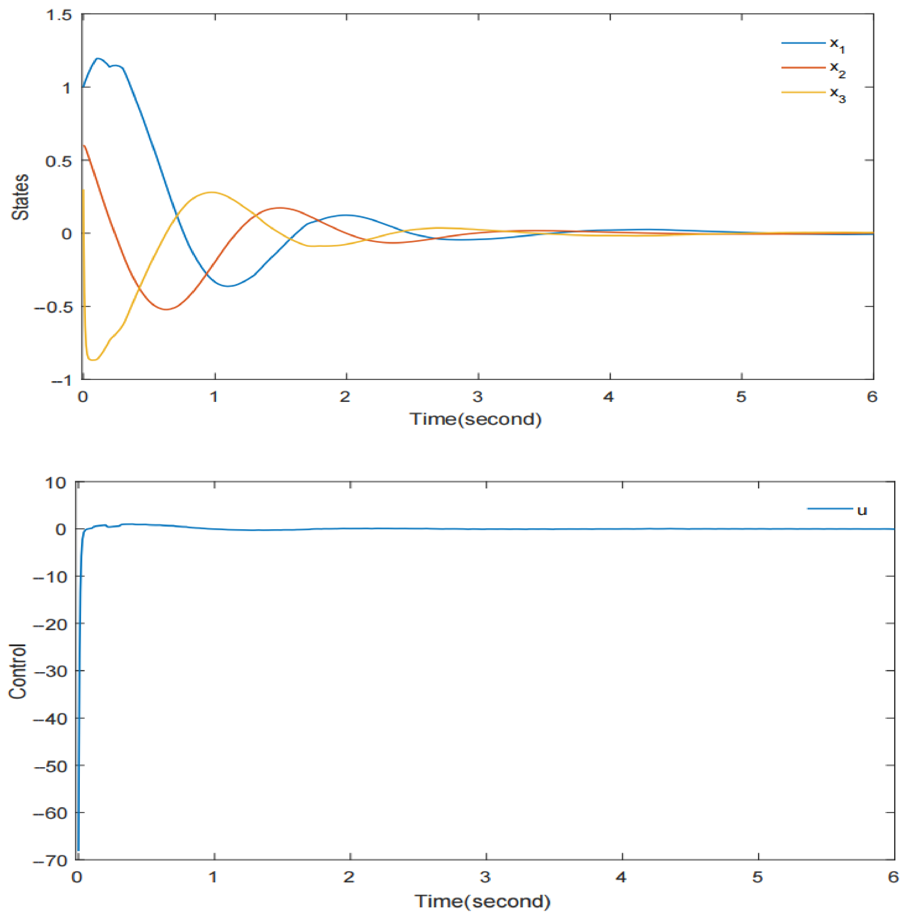
4. A Simulation Example

In this section, a numerical example is used to verify the rationality and validity of the results in Section 3.

Suppose that the following system is taken for simulation:

$$\begin{array}{cc}\hfill d{x}_1& =\left((5+0.1sint)x_2+x_3{cos}^2{x}_3\right)dt+x_{3}cos{x}_{3}d\omega ,\hfill \\ \hfill d{x}_2& =(3+2sint)x_{3}dt,\hfill \\ \hfill d{x}_3& =(2+0.5sint)udt.\hfill \end{array}$$

(43)

Obviously, the system satisfies Assumption 1. Notice that there exist normal numbers ${\lambda }_i$, ${\mu }_i(i=1,2,3)$, and $\mu$, with ${\lambda }_1\le 4.9\le d_1\left(t\right)\le 5.1\le {\mu }_1\le \mu$, ${\lambda }_2\le 1\le d_2\left(t\right)\le 5\le {\mu }_2\le \mu$ and ${\lambda }_3\le 1.5\le d_3\left(t\right)\le 2.5\le {\mu }_3\le \mu$, which satisfy Assumption 2.

Inputting the coordinates

$$\begin{array}{c}\hfill z_1=x_1,z_2=\frac{x_2}{\epsilon },z_3=\frac{x_3}{{\epsilon }^2},v=\frac{u}{{\epsilon }^3},\end{array}$$

(44)

where $0<\epsilon <1$ is an undetermined parameter, system (43) could be rewritten as

$$\begin{array}{cc}\hfill d{z}_1& =\left(\epsilon (5+0.1sint)z_2+{\epsilon }^2{z}_3{cos}^2{\epsilon }^2{z}_3\right)dt+{\epsilon }^2{z}_{3}cos{\epsilon }^2{z}_{3}d\omega ,\hfill \\ \hfill d{z}_2& =\epsilon (3+2sint)z_{3}dt,\hfill \\ \hfill d{z}_3& =\epsilon (2+0.5sint)vdt.\hfill \end{array}$$

(45)

According to the design process above, the controller can be obtained as follows:

$$\begin{array}{c}\hfill v=-598(60z_1+4z_2+z_3).\end{array}$$

(46)

By (44), we can get the controller as follows:

$$\begin{array}{c}\hfill u=-598(60{\epsilon }^3{x}_1+4{\epsilon }^2{x}_2+\epsilon x_3).\end{array}$$

(47)

The simulation is performed by selecting $\epsilon =0.1$, $x_1\left(0\right)=1$, $x_2\left(0\right)=0.6$, and $x_3\left(0\right)=0.3$. Figure 1 illustrates the responses of the closed-loop systems (43)–(47) and verifies the effectiveness of the controller.

Remark 5.

The simulation shows only a numerical example, not a real example. As can be seen in Figure 1, under the designed controller, the response curves of the closed-loop system almost certainly converge to zero. In general, when there is a time-varying coefficient, the controller designed based on the backstepping technique and the low-gain homogeneous domination technology has a better performance, so it is of great significance in practical applications. Now that we know the importance of physical models, finding a real-world mechanical device that can be modeled directly with system (2) or that can be transformed into a system (2) through coordinate transformation is a top priority for future research.

Remark 6.

It should be further noted that the difference between this paper and other papers is that this is a theoretical study that provides a new idea for solving the state feedback stabilization problem of trigonometric stochastic nonlinear systems with time-varying control coefficients.

5. Conclusions

The state feedback control problem is studied in this article by utilizing the backstepping technique, the low-gain homogeneous domination technique, and some significant inequalities. The systems are considered to be upper-triangular stochastic nonlinearities, and the control coefficients are uncertain. The designed controller is able to ensure that the closed-loop system is GAS almost everywhere. Based on these, there are some associated issues that could be researched more in the future. For instance, the extension of this control strategy to more general systems, such as high-order stochastic systems, should be considered. A practical example for system (2) for simulation verification should also be found. The results of fixed points in b-Metric Space can then be considered for stochastic nonlinear systems [45,46].

References

1. Wang, Y.H.; Zhang, T.L.; Zhang, W.H. Feedback stabilization for a class of nonlinear stochastic systems with state- and control-dependent noise. Math. Probl. Eng. 2014, 2014, 484732. [Google Scholar] [CrossRef]
2. Tian, J.; Xie, X.J. Adaptive state-feedback stabilization for high-order stochastic non-linear systems with uncertain control coefficients. Int. J. Control 2007, 80, 1503–1516. [Google Scholar] [CrossRef]
3. Cui, R.H.; Xie, X.J. Adaptive state-feedback stabilization of state-constrained stochastic high-order nonlinear systems. Sci. China Inf. Sci. 2021, 64, 200203. [Google Scholar] [CrossRef]
4. Ku, C.C.; Yeh, Y.C.; Lin, Y.H.; Hsieh, Y.Y. Fuzzy static output control of T-S fuzzy stochastic systems via line integral Lyapunov function. Processes 2021, 9, 697. [Google Scholar] [CrossRef]
5. Li, W.Q.; Yao, X.X.; Krstic, M. Adaptive-gain observer-based stabilization of stochastic strict-feedback systems with sensor uncertainty. Automatica 2020, 120, 109112. [Google Scholar] [CrossRef]
6. Li, W.Q.; Krstic, M. Stochastic adaptive nonlinear control with filterless least-squares. IEEE Trans. Autom. Control 2021, 66, 3893–3905. [Google Scholar] [CrossRef]
7. Li, W.Q.; Krstic, M. Mean-nonovershooting control of stochastic nonlinear systems. IEEE Trans. Autom. Control 2021, 66, 5756–5771. [Google Scholar] [CrossRef]
8. Li, W.Q.; Krstic, M. Stochastic nonlinear prescribed-time stabilization and inverse optimality. IEEE Trans. Autom. Control 2022, 67, 1179–1193. [Google Scholar] [CrossRef]
9. Li, W.Q.; Krstic, M. Prescribed-time output-feedback control of stochastic nonlinear systems. IEEE Trans. Autom. Control 2022, 63, 1. [Google Scholar] [CrossRef]
10. Fotakis, J.; Grimble, M.; Kouvaritakis, B. A comparison of characteristic locus and optimal designs for dynamic ship positioning systems. IEEE Trans. Autom. Control 1982, 27, 1143–1157. [Google Scholar] [CrossRef]
11. From, P.J.; Gravdahl, J.T.; Lillehagen, T.; Abbeel, P. Motion planning and control of robotic manipulators on seaborne platforms. Control Eng. Pract. 2011, 19, 809–819. [Google Scholar] [CrossRef]
12. Sun, X.Y.; Gao, Y.; Liu, Q.S. Event-triggered communication scheme for stochastic systems in wireless sensor networks. J. Algorithms Comput. 2020, 14, 1748302620907542. [Google Scholar]
13. Jiang, X.S.; Tian, S.P.; Zhang, T.L.; Zhang, W.H. Stability and stabilization of nonlinear discrete-time stochastic systems. Int. J. Robust Nonlinear 2019, 29, 6419–6437. [Google Scholar] [CrossRef]
14. Jiang, M.M.; Xie, X.J. State feedback stabilization of stochastic nonlinear time-delay systems: A dynamic gain method. Sci. China Inf. Sci. 2020, 64, 119202. [Google Scholar] [CrossRef]
15. Jiang, X.S.; Zhao, D.Y. Event-triggered fault detection for nonlinear discrete-time switched stochastic systems: A convex function method. Sci. China Inf. Sci. 2021, 64, 200204. [Google Scholar] [CrossRef]
16. Li, W.Q.; Liu, L.; Feng, G. Cooperative control of multiple nonlinear benchmark systems perturbed by second-order moment processes. IEEE Trans. Cybern. 2020, 50, 902–910. [Google Scholar] [CrossRef]
17. Li, W.Q.; Liu, L.; Feng, G. Distributed output-feedback tracking of multiple nonlinear systems with unmeasurable states. IEEE Trans. Syst. Man Cybern. Syst. 2021, 51, 477–486. [Google Scholar] [CrossRef]
18. Fang, L.D.; Ding, S.H.; Park, J.H.; Ma, L. Adaptive fuzzy output-feedback control design for a class of p-norm stochastic nonlinear systems with output constraints. IEEE Trans. Circuits-I 2021, 68, 2626–2638. [Google Scholar] [CrossRef]
19. Ku, C.C.; Chang, W.J.; Huang, K.W. Novel delay-dependent stabilization for fuzzy stochastic systems with multiplicative noise subject to passivity constraint. Processes 2021, 9, 1445. [Google Scholar] [CrossRef]
20. Pan, Z.G.; Basar, T. Adaptive controller design for tracking and disturbance attenuation in parametric strict-feedback nonlinear systems. IEEE Trans. Autom. Control 1998, 43, 1066–1083. [Google Scholar] [CrossRef]
21. Pan, Z.G.; Basar, T. Backstepping controller design for nonlinear stochastic systems under a risk-sensitive cost criterion. SIAM J. Control Optim. 1999, 37, 957–995. [Google Scholar] [CrossRef]
22. Krstic, M.; Deng, H. Stabilization of Uncertain Nonlinear Systems; Springer: New York, NY, USA, 1998. [Google Scholar]
23. Deng, H.; Krstic, M.; Williams, R.J. Stabilization of stochastic nonlinear systems driven by noise of unknown covariance. IEEE Trans. Autom. Control 2001, 46, 1237–1253. [Google Scholar] [CrossRef] [Green Version]
24. Deng, H.; Krstic, M. Output-feedback stochastic nonlinear stabilization. IEEE Trans. Autom. Control 1999, 44, 328–333. [Google Scholar] [CrossRef] [Green Version]
25. Chen, W.S.; Jiao, L.C.; Li, J. Adaptive NN backstepping out-feedback control for stochastic nonlinear strict-feedback systems with time-varying delays. IEEE Trans. Cybern. 2010, 40, 939–950. [Google Scholar] [CrossRef] [PubMed]
26. Liu, L.; Yin, S.; Gao, H. Adaptive partial-state feedback control for stochastic high-order stochastic nonlinear systems with stochastic input-to-state stable inverse dynamics. Automatica 2015, 47, 2772–2779. [Google Scholar] [CrossRef]
27. Cui, R.H.; Xie, X.J. Finite-time stabilization of stochastic low-order nonlinear systems with time-varying orders and FT-SISS inverse dynamics. Automatica 2021, 125, 109418. [Google Scholar] [CrossRef]
28. Cui, R.H.; Xie, X.J. Finite-time stabilization of output-constrained stochastic high-order nonlinear systems with high-order and low-order nonlinearities. Automatica 2022, 136, 110085. [Google Scholar] [CrossRef]
29. Li, J.; Qian, C.J. Global finite-time stabilization of a class of uncertain nonlinear systems using output feedback. In Proceedings of the 44th IEEE Conference on Decision and Control and the European Control Conference, Seville, Spain, 12–15 December 2005; pp. 2652–2657. [Google Scholar]
30. Lan, Q.X.; Li, S.H. Global output-feedback stabilization for a class of stochastic nonlinear systems via sampled-data control. Int. J. Robust Nonlinear 2017, 27, 3643–3658. [Google Scholar] [CrossRef]
31. Wu, Z.H.; Deng, F.Q.; Guo, B.Z.; Wu, C.F.; Xiang, Q.M. Backstepping active disturbance rejection control for lower triangular nonlinear systems with mismatched stochastic disturbances. IEEE Trans. Syst. Man Cybern. Syst. 2021, 52, 2688–2702. [Google Scholar] [CrossRef]
32. Mazenc, F.; Bowong, S. Tracking trajectories of the cart-pendulum system. Automatica 2003, 39, 677–684. [Google Scholar] [CrossRef]
33. Teel, A.R. A nonlinear small gain theorem for the analysis of control systems with saturation. IEEE Trans. Autom. Control 1996, 41, 1256–1270. [Google Scholar] [CrossRef]
34. Zha, W.T.; Zhai, J.Y.; Fei, S.M.; Wang, Y.J. Finite-time stabilization for a class of stochastic nonlinear systems via output feedback. ISA Trans. 2014, 53, 709–716. [Google Scholar] [CrossRef]
35. Qian, C.J.; Li, J. Global output feedback stabilization of upper-triangular nonlinear systems using a homogeneous domination approach. Int. J. Robust Nonlinear 2006, 16, 441–463. [Google Scholar] [CrossRef]
36. Li, W.Q.; Jing, Y.W.; Zhang, S.Y. State-feedback stabilization of a class of upper-triangular stochastic nonlinear systems. Control Decis. 2010, 25, 1543–1546. [Google Scholar]
37. Liu, L.; Zhang, Y.F. Decentralised output-feedback control for a class of large-scale stochastic high-order upper-triangular nonlinear systems. Int. J. Syst. Sci. 2016, 48, 838–848. [Google Scholar] [CrossRef]
38. Liu, L.; Xing, X.; Gao, M. Global stabilization for a class of stochastic high-order feedforward nonlinear systems via homogeneous domination approach. Circuits Syst. Signal Process. 2016, 35, 2723–2740. [Google Scholar] [CrossRef]
39. Bao, X.Y.; Wang, H.; Li, W.Q. Containment control for upper-triangular nonlinear multi-agent systems perturbed by second-order moment processes. IEEE Access 2021, 9, 21102–21111. [Google Scholar] [CrossRef]
40. Zhang, T.L.; Deng, F.Q.; Sun, Y.; Shi, P. Fault estimation and fault-tolerant control for linear discrete time-varying stochastic systems. Sci. China Inf. Sci. 2021, 64, 200201. [Google Scholar] [CrossRef]
41. Zhang, X.F.; Chen, Z.L. Output-feedback stabilization of nonlinear systems with delays in the input. Appl. Math. Comput. 2005, 167, 1026–1040. [Google Scholar] [CrossRef]
42. Du, H.B.; Qian, C.J.; He, Y.G. Global sampled-data output feedback stabilization of a class of upper-triangular systems with input delay. IET Control Theory Appl. 2013, 7, 1437–1446. [Google Scholar] [CrossRef]
43. Liu, L.; Gao, M. State feedback control for stochastic feedforward nonlinear systems. Math. Probl. Eng. 2013, 2013, 908459. [Google Scholar] [CrossRef]
44. Zhao, C.R.; Xie, J.X. Global stabilization of stochastic high-order feedforward nonlinear systems with time-varying delay. Automatica 2014, 50, 203–210. [Google Scholar] [CrossRef]
45. Rasham, T.; Shoaib, A.; Hussain, N.; Alamri, B.A.S.; Arshad, M. Multivalued fixed point results in dislocated b-metric spaces with application to the system of nonlinear integral equations. Symmetry 2019, 11, 40. [Google Scholar] [CrossRef] [Green Version]
46. Rasham, T.; Marino, G.; Shahzad, A.; Park, C.; Shoaib, A. Fixed point results for a pair of fuzzy mappings and related applications in b-metric like spaces. Adv. Differ. Equ. 2021, 2021, 259. [Google Scholar] [CrossRef]
47. Lin, W.; Qian, C. Adding one power integrator: A tool for global stabilization of high-order lower-triangular systems. Syst. Control Lett. 2000, 39, 339–351. [Google Scholar] [CrossRef]
Figure 1. The responses of a closed-loop system.
Processes 10 01465 g001
Publisher’s Note: MDPI stays neutral with regard to jurisdictional claims in published maps and institutional affiliations.