Pareto Optimal Strategy under H_∞ Constraint for Discrete-Time Stochastic Systems

Abstract

This paper investigates the Pareto optimal strategy of discrete-time stochastic systems under $H_{\infty }$ constraint, in which the weighting matrices of the weighted sum cost function can be indefinite. Combining the $H_{\infty }$ control theory with the indefinite LQ control theory, the generalized difference Riccati equations (GDREs) are obtained. By means of the solution of the GDREs, the Pareto optimal strategy with $H_{\infty }$ constraint is derived, and the necessary and sufficient conditions for the existence of the strategy are presented. Then the Pareto optimal solution under the worst-case disturbance is solved. Finally, the efficiency of the obtained results is illustrated by a numerical example.

1. Introduction

With the increasing scale of modern industry and economy, it is unavoidable to deal with multi-player and multi-objective optimal control problems [1]. There will inevitably be cooperation or competition between different players. As an important tool to solve this problem, game theory has been widely studied by scholars [2,3,4,5]. Game theory includes the noncooperative game and the cooperative game. In a noncooperative game, one player makes independent decisions without considering the benefits of the other players. On the contrary, the cooperative game reasonably coordinates the interests of each player within a specific rule. As the concept of win-win cooperation gains popularity, the cooperative game has also become a popular topic.

As an important type of cooperative games, Pareto game has firstly been used in economic theories [6,7], and now it is also used in the engineering field, such as path planning [8], crude oil scheduling [9] and mobile edge computing [10]. Hence, Pareto game has been widely investigated by many researchers. Engwerda [11] gave a characterization of all Pareto solutions when the weighting matrices of the cost function are positive definite and then generalized this result for indefinite criteria [12]. Further, Reddy [13] studied the conditions for the existence of Pareto optimal strategy in infinite horizon, and systematically analyzed the relationship between Pareto optimality and weight sum minimization. Along with maturing of Pareto optimal control theory for deterministic systems, scholars have done some work on Pareto optimal control of stochastic systems. Lin et al. [14] derived the necessary and sufficient conditions for Pareto optimal strategy of stochastic system. For discrete-time stochastic systems, Zhu et al. [15] gave sufficient conditions for the existence of the strategy sets with finite horizon, and Peng et al. [16,17] studied the Pareto optimality of linear and nonlinear systems with infinite horizon, respectively. Ahmed et al. [18] studied the Pareto optimal control with external disturbances, and gave the form of Pareto optimal control under $H_{\infty }$ constraint for continuous-time stochastic systems by means of linear matrix inequalities. Jiang et al. [19] introduced the generalized differential Riccati equations to obtain Pareto solutions under $H_{\infty }$ constraint for continuous-time stochastic systems. It should be noted that the above two articles are about continuous-time rather than discrete-time.

The development of Pareto optimal control theory is inseparable from the progress of linear quadratic (LQ) dynamic game theory. The stochastic LQ optimal control problem was proposed initially by Wonham [20] and attracted great attention of many scholars [21,22,23]. Chen et al. [24] found that a stochastic LQ problem with indefinite cost weighting matrices can still be well-posed. The reference [25] investigated discrete-time indefinite stochastic LQ problem and proposed a generalized difference Riccati equation (GDRE). To design optimal robust controllers with external disturbances, in [26], the authors proposed the mixed $H_2/H_{\infty }$ control, while [27] generalized $H_2/H_{\infty }$ control theory of deterministic systems to stochastic systems. However, different from the Pareto optimal control studied in this paper, $H_2/H_{\infty }$ control can only give the optimal control of single-player, and can not deal with the optimization problem of multi-player and multi-objective.

Compared with the $H_2/H_{\infty }$ control, there are few studies on the Pareto efficiency with $H_{\infty }$ constraint for discrete-time stochastic systems. However, practical systems are often affected by both white noises and exogenous disturbances, and compared with the generalized differential Riccati equations, it is easier to solve the GDREs associated with discrete-time stochastic systems. In recent years, the characteristics of discrete stochastic systems have become a very attractive research field [28,29]. Motivated by the above discussions, we study the Pareto optimum for stochastic discrete-time systems with external disturbances. The main contributions of this work are as follows:

• Using the weighted sum method of Pareto optimization and combined with the $H_{\infty }$ control theory, the GDREs are obtained. Based on obtained GDREs, we get the Pareto efficient strategies under $H_{\infty }$ constraint, which can not only achieve Pareto optimization, but also reduce the influence of external disturbances.
• Based on the solvability of the GDREs, we derive the necessary and the sufficient conditions for the existence of $H_{\infty }$ constraint Pareto optimal control for discrete-time stochastic systems. Then we derive all Pareto solutions for all Pareto efficient strategies.
• We investigate the indefinite linear-quadratic difference game with external disturbance and stochastic bounded real lemma (SBRL) with a nonzero initial value. The weighting matrices of the cost functional are allowed to be indefinite in this paper.

The rest of this paper is organized as follows: Section 2 presents the system description and makes some useful preliminaries. In Section 3, Pareto optimality under $H_{\infty }$ constraint is investigated. Section 4 presents an example of space heating to illustrate the obtained results. The conclusion of this paper is given in Section 5.

Notations: ${\mathcal{A}}^{\prime }$: the transpose of the matrix or vector $\mathcal{A}$; ${\mathcal{A}}^{†}$: the Moore-Penrose pseudoinverse of $\mathcal{A}$; $\mathcal{A}>0(\mathcal{A}⩾0)$: $\mathcal{A}$ is the positive definite (positive semi-definite) symmetric matrix; $\mathbb{E}(·)$: the mathematical expectation operator; ${\mathcal{R}}^n$: the set of n-dimensional real vectors; ${\mathcal{R}}^{m\times n}$: the set of $m\times n$ real matrices; ${\mathcal{I}}_n$: the $n\times n$ identity matrix; ${\mathcal{S}}_n$: the set of all $n\times n$ real symmetric matrices; ${\mathcal{N}}_T:=\{0,1,2,\dots ,T\}$; $col(\mathcal{A},\mathcal{B}):=\left[\begin{array}{c}\mathcal{A}\\ \mathcal{B}\end{array}\right];$$\mathcal{N}:=\{1,2,\dots ,N\}.$

2. System Descriptions and Preliminaries

Consider stochastic finite horizon discrete-time linear system with multi-player as follows:

$$\left\{\begin{array}{c}{x}_{k+1}={\mathcal{A}}_k{x}_k+\sum _{i=1}^N{\mathcal{B}}_{i,k}{u}_{i,k}+{\mathcal{C}}_k{v}_k+{\mathcal{D}}_k{x}_k{w}_k+\sum _{i=1}^N{\mathcal{Z}}_{i,k}{u}_{i,k}{w}_k+{\mathcal{F}}_k{v}_k{w}_k,\hfill \\ z_k=\left[\begin{array}{c}{\mathcal{W}}_k{x}_k\\ {\mathcal{G}}_{1,k}{u}_{1,k}\\ ⋮\\ {\mathcal{G}}_{N,k}{u}_{N,k}\end{array}\right],x_0\in {\mathcal{R}}^n,k\in {\mathcal{N}}_T:=\{0,1,2,\dots ,T\},\hfill \end{array}\right.$$

(1)

where $x_k\in {\mathcal{R}}^n$ represents the system state, $u_{i,k}\in {\mathcal{R}}^{m_i}$ is the ith control input at time k, $v_k\in {\mathcal{R}}^{n_v}$ is the disturbance signal, $z_k\in {\mathcal{R}}^{n_z}$ is the controlled output. Denote the joint action of each controllers by $u_k:=col(u_{1,k},\dots ,u_{N,k})\in {\mathcal{R}}^m,m={\sum }_{i=1}^N{m}_i$. ${\mathcal{A}}_k$, ${\mathcal{B}}_{i,k}$, ${\mathcal{C}}_k$, ${\mathcal{D}}_k$, ${\mathcal{Z}}_{i,k}$, ${\mathcal{F}}_k$, ${\mathcal{W}}_k$ and ${\mathcal{G}}_{i,k}$ with $i=1,2,\dots ,N$ are matrix-valued continuous functions with appropriate dimensions. ${\left\{w_k\right\}}_{k\in {\mathcal{N}}_T}$ is an independent one-dimensional real random variable sequence defined in a given complete filtered probability space $\{\mathsf{\Omega },\mathcal{F},{\mathcal{F}}_k,\mathcal{P}\}$ with $\mathbb{E}\left(w_k\right)=0$ and $\mathbb{E}\left(w_k{w}_s\right)={\delta }_{sk}$, where ${\delta }_{sk}$ is a Kronecker function. Denote ${\mathcal{F}}_k=\sigma \left(w_s:s\in {\mathcal{N}}_k\right)$ the $\sigma$ -algebra generated by $w_k,k\in {\mathcal{N}}_T.$ Let $l_w^2\left({\mathcal{N}}_T,{\mathcal{R}}^k\right)$ consists of all finite sequences $f={\left\{f_i:f_i\in {\mathcal{R}}^k\right\}}_{0⩽i⩽T}$$=\{f_0,f_1,\dots ,f_T\}$, such that $f_i$ is ${\mathcal{F}}_{i-1}$ measurable for $i\in {\mathcal{N}}_T$, where ${\mathcal{F}}_{-1}=\{\varphi ,\mathsf{\Omega }\}$, i.e., $f_0$ is constant. The $l^2$-norm of $f\in l_w^2\left({\mathcal{N}}_T,{\mathcal{R}}^k\right)$ is defined as

$${\parallel f\parallel }_{l_w^2\left({\mathcal{N}}_T,{\mathcal{R}}^k\right)}={\left(\sum _{k=0}^T\mathbb{E}{\parallel f_k\parallel }^2\right)}^{1/2}.$$

Before giving the definition of Pareto optimal strategy with $H_{\infty }$ constraint, we need to analyze the Pareto optimality and $H_{\infty }$ performance of discrete-time systems, respectively. We will first introduce some definitions and lemmas of Pareto optimal strategy. In this part, the disturbance is not considered. Let $v_k\equiv 0$, system (1) can be reduced to

$$\left\{\begin{array}{c}{x}_{k+1}={\mathcal{A}}_k{x}_k+\sum _{i=1}^N{\mathcal{B}}_{i,k}{u}_{i,k}+{\mathcal{D}}_k{x}_k{w}_k+\sum _{i=1}^N{\mathcal{Z}}_{i,k}{u}_{i,k}{w}_k,\hfill \\ z_k=\left[\begin{array}{c}{\mathcal{W}}_k{x}_k\\ {\mathcal{G}}_{1,k}{u}_{1,k}\\ ⋮\\ {\mathcal{G}}_{N,k}{u}_{N,k}\end{array}\right],x_0\in {\mathcal{R}}^n,k\in {\mathcal{N}}_T.\hfill \end{array}\right.$$

(2)

For system (2), the cost functionals that the player or controller $u_{i,k}$ wants to minimize are

$${\mathcal{J}}_i\left(u_{1,k},\dots ,u_{N,k};x_0\right):=\sum _{k=0}^T\mathbb{E}\left(x_k^{\prime }{\mathcal{Q}}_i{x}_k+\sum _{j=1}^N{u}_{j,k}^{\prime }{\mathcal{R}}_{ij}{u}_{j,k}\right),$$

(3)

where $i,j\in \mathcal{N}$, ${\mathcal{Q}}_i,{\mathcal{R}}_{ij}\in {\mathcal{S}}_n$ and ${\mathcal{R}}_{ij}^{-1}$ exists.

Definition 1

([19]). Denote ${\mathcal{J}}_i\left(u,x_0\right)={\mathcal{J}}_i\left(u_{1,k},\dots ,u_{N,k};x_0\right)$ and joint control $u:=(u_{1,k},\dots ,$$u_{N,k})\in \mathcal{U}$, where $\mathcal{U}$ is the set of all admissible controls. The $u^{*}$ is called Pareto efficient for system (2), if the set of the inequalities ${\mathcal{J}}_i\left(u,x_0\right)\le {\mathcal{J}}_i\left(u^{*},x_0\right)$, $i\in \mathcal{N}:=\{1,2,\dots ,N\}$ do not hold for any solution $u\in \mathcal{U}$, where at least one of the inequalities is strict. The $\left({\mathcal{J}}_1\left(u^{*},x_0\right),\dots ,{\mathcal{J}}_N\left(u^{*},x_0\right)\right)$ corresponding to Pareto efficiency $u^{*}$ is a Pareto solution, and all Pareto solutions form the Pareto frontier.

If $u^{*}$ is Pareto efficient, it means that we cannot find other admissible u to make one or more ${\mathcal{J}}_i(u,x_0),i\in \mathcal{N}$ get better while no ${\mathcal{J}}_j(u,x_0),j\in \mathcal{N}\text{}i$ gets worse at the same time. To solve pareto efficiency, we need to introduce the following two lemmas.

Lemma 1

([30]). Let $\alpha =\left({\alpha }_1,\dots ,{\alpha }_N\right)\in \mathbb{A}$, where

$$\mathbb{A}:=\left\{\alpha =\left({\alpha }_1,\dots ,{\alpha }_N\right)\mid 0\le {\alpha }_i\le 1and\sum _{i=1}^N{\alpha }_i=1\right\}.$$

Assume $u^{*}\in \mathcal{U}$ such that

$$u^{*}\in arg\underset{u\in \mathcal{U}}{min}\left\{\sum _{i=1}^N{\alpha }_i{\mathcal{J}}_i\left(u,x_0\right)\right\}.$$

(4)

Then $u^{*}$ is Pareto efficient.

Lemma 2

([12]). Assume that the control strategy set $\mathcal{U}$ is a convex set and the cost functionals ${\mathcal{J}}_i\left(u,x_0\right),i\in \mathcal{N}$, are convex w.r.t. u. If admissible $u^{*}$ is Pareto efficient, then there exists an $\alpha =\left({\alpha }_1,\dots ,{\alpha }_N\right)\in \mathbb{A}$ such that $\left(4\right)$ holds.

Remark 1.

Lemma 1 is only a sufficient condition to obtain Pareto efficient strategies, and it cannot guarantee that all Pareto efficient strategies can be obtained by (4). If ${\mathcal{Q}}_i⩾0$ and ${\mathcal{R}}_{ij}>0,$$i,j\in \mathcal{N}$,through triangle inequality [11], we can infer that the corresponding cost functionals ${\mathcal{J}}_i,i\in \mathcal{N}$ are convex. According to Lemma 2, if the control strategy set $\mathcal{U}$ and the cost functionals ${\mathcal{J}}_i,i\in \mathcal{N}$ are convex, the Pareto efficient strategy $u^{*}$ can be obtained by the weighted sum method. In this paper, we consider the case that ${\mathcal{Q}}_i$ and ${\mathcal{R}}_{ij}$ may be indefinite matrices, which requires us first to ensure that ${\mathcal{J}}_i$ is convex.

Lemma 3

([14]). Consider the system (2). The cost functionals ${\mathcal{J}}_i\left(u,x_0\right)$ shown in Equation (3) is convex w.r.t. $u\in \mathcal{U}$, where $\mathcal{U}$ is a convex set, iff ${min}_{u\in \mathcal{U}}{J}_i(u,0)=0,i\in \mathcal{N}.$

Under the assumption that $u\in \mathcal{U}$ is convex and ${min}_{u\in \mathcal{U}}{J}_i(u,0)=0,i\in \mathcal{N}$, the convexity of the cost function is guaranteed, which further ensures that all Pareto efficient strategies with indefinite matrices ${\mathcal{Q}}_i$ and ${\mathcal{R}}_{ij}$ can be obtained by minimizing the weighted cost functional.

For the weighted sum cost functional

$$\begin{array}{c}\hfill {\mathcal{J}}_{\alpha }\left(u,x_0\right)=\sum _{i=1}^N{\alpha }_j{\mathcal{J}}_i\left(u_{1,k},\dots ,u_{N,k};x_0\right):=\sum _{k=0}^T\mathbb{E}\left(x_k^{\prime }{\mathcal{Q}}_{\alpha }{x}_k+\sum _{j=1}^N{u}_{j,k}^{\prime }{\mathcal{R}}_{\alpha }{u}_{j,k}\right),\end{array}$$

(5)

if ${\mathcal{J}}_i\left(u,x_0\right),i\in \mathcal{N}$ are all convex w.r.t. u, then the corresponding ${\mathcal{J}}_{\alpha }\left(u,x_0\right)$ is also convex for any $\alpha \in \mathbb{A}$, ${\mathcal{R}}_{\alpha }={\sum }_{i=1}^N{\alpha }_i{\mathcal{R}}_i$, ${\mathcal{R}}_i=diag\left\{{\mathcal{R}}_{i1},\dots ,{\mathcal{R}}_{iN}\right\}$, ${\mathcal{Q}}_{\alpha }={\sum }_{i=1}^N{\alpha }_i{\mathcal{Q}}_i$.

Next, let control input $u\equiv 0$ consider the following discrete-time stochastic perturbed system for $H_{\infty }$ analysis.

$$\left\{\begin{array}{c}{x}_{k+1}={\mathcal{A}}_k{x}_k+{\mathcal{C}}_k{v}_k+{\mathcal{D}}_k{x}_k{w}_k+{\mathcal{F}}_k{v}_k{w}_k,\hfill \\ z_k={\mathcal{W}}_k{x}_k,x_0\in {\mathcal{R}}^n,k\in {\mathcal{N}}_T.\hfill \end{array}\right.$$

(6)

The perturbed operator of system (6) is defined by ${\mathcal{L}}_T:l_w^2\left({\mathcal{N}}_T,{\mathcal{R}}^{n_v}\right)\to l_w^2\left({\mathcal{N}}_T,{\mathcal{R}}^{n_z}\right)$ with ${\mathcal{L}}_T(v_k,x_0)=z_k$, $k\in {\mathcal{N}}_T,$$v_k\in l_w^2\left({\mathcal{N}}_T,{\mathcal{R}}^{n_v}\right).$ Define the norm of the perturbed operator of system (6) as

$$\begin{array}{cc}\hfill ∥{\overline{\mathcal{L}}}_T∥:=& \underset{v\in l_w^2\left({\mathcal{N}}_T,{\mathcal{R}}^{n_v}\right),v\ne 0}{sup}\frac{\parallel z_k{\parallel }_{l_w^2\left({\mathcal{N}}_T,{\mathcal{R}}^{n_z}\right)}}{{\left({∥{\mathcal{S}}^{1/2}{x}_0∥}^2+{\parallel v_k\parallel }_{l_w^2\left({\mathcal{N}}_T,{\mathcal{R}}^{n_v}\right)}^2\right)}^{1/2}}\hfill \\ \hfill =& \underset{v\in l_w^2\left({\mathcal{N}}_T,{\mathcal{R}}^{n_v}\right),v\ne 0}{sup}\frac{{\left[{\sum }_{k=0}^T\mathbb{E}\left(x_k^{\prime }{\mathcal{W}}_k^{\prime }{\mathcal{W}}_k{x}_k\right)\right]}^{1/2}}{{\left(x_0^{\prime }\mathcal{S}{x}_0+{\sum }_{k=0}^T\mathbb{E}{\parallel v_k\parallel }^2\right)}^{1/2}}.\hfill \end{array}$$

(7)

In (7) the initial weighting matrix $\mathcal{S}={\mathcal{S}}^{\prime }>0$ is introduced to measure the uncertainty of initial state $x_0$. It can be seen that $∥{\overline{\mathcal{L}}}_T∥$ represents the effect of the initial value and external disturbance on the system output. When we require $∥{\overline{\mathcal{L}}}_T∥<\gamma$, the following robust cost functional is obtained, which establishes a relationship between the disturbance attenuation problem and the solvability of GDRE.

$${\mathcal{J}}_v\left(v,x_0\right):=\sum _{k=0}^T\mathbb{E}\left({\gamma }^2\parallel v_k{\parallel }^2-{\parallel z_k\parallel }^2\right)+{\gamma }^2{x}_0^{\prime }\mathcal{S}{x}_0.$$

(8)

For notational convenience, simplify discrete-time system (1) as

$$\left\{\begin{array}{c}{x}_{k+1}={\mathcal{A}}_k{x}_k+{\mathcal{B}}_k{u}_k+{\mathcal{C}}_k{v}_k+{\mathcal{D}}_k{x}_k{w}_k+{\mathcal{Z}}_k{u}_k{w}_k+{\mathcal{F}}_k{v}_k{w}_k,\hfill \\ z_k=\left[\begin{array}{c}{\mathcal{W}}_k{x}_k\\ {\mathcal{G}}_k{u}_k\end{array}\right],x_0\in {\mathcal{R}}^n,k\in {\mathcal{N}}_T,\hfill \end{array}\right.$$

(9)

where ${\mathcal{B}}_k:=[{\mathcal{B}}_{1,k}{\mathcal{B}}_{2,k}···{\mathcal{B}}_{N,k}]$, ${\mathcal{Z}}_k:=[{\mathcal{Z}}_{1,k}{\mathcal{Z}}_{2,k}···{\mathcal{Z}}_{N,k}]$, ${\mathcal{G}}_k:=\left[\begin{array}{cccc}{\mathcal{G}}_{1,k}& 0& \cdots & 0\\ 0& {\mathcal{G}}_{2,k}& \cdots & 0\\ ⋮& ⋮& \cdots & ⋮\\ 0& 0& \cdots & {\mathcal{G}}_{N,k}\end{array}\right]$

Based on the above analysis, we define the Pareto optimal strategy for discrete-time system (9) with $H_{\infty }$ constraint.

Definition 2.

Consider the controlled stochastic system (9). For a given disturbance attenuation level $\gamma >0$, find a state feedback joint control $u^{*}$ with $u_k^{*}={\mathcal{K}}_k{x}_k$, such that

(1) For the closed-loop system

$$\left\{\begin{array}{c}{x}_{k+1}=({\mathcal{A}}_k+{\mathcal{B}}_k{\mathcal{K}}_k)x_k+{\mathcal{C}}_k{v}_k+({\mathcal{D}}_k+{\mathcal{Z}}_k{\mathcal{K}}_k)x_k{w}_k+{\mathcal{F}}_k{v}_k{w}_k,\hfill \\ z_k=\left[\begin{array}{c}{\mathcal{W}}_k{x}_k\\ {\mathcal{G}}_k{\mathcal{K}}_k{x}_k\end{array}\right],x_0\in {\mathcal{R}}^n,k\in {\mathcal{N}}_T,\hfill \end{array}\right.$$

(10)

the norm of the perturbed operator of (10) satisfies

$$\begin{array}{cc}\hfill ∥{\mathcal{L}}_T∥& :=\underset{v\in l_w^2\left({\mathcal{N}}_T,{\mathcal{R}}^{n_v}\right),v\ne 0}{sup}\frac{\parallel z_k{\parallel }_{l_w^2\left({\mathcal{N}}_T,{\mathcal{R}}^{n_z}\right)}}{{\left({∥{\mathcal{S}}^{1/2}{x}_0∥}^2+{\parallel v_k\parallel }_{l_w^2\left({\mathcal{N}}_T,{\mathcal{R}}^{n_v}\right)}^2\right)}^{1/2}}\hfill \\ \hfill & =\underset{v\in l_w^2\left({\mathcal{N}}_T,{\mathcal{R}}^{n_v}\right),v\ne 0}{sup}\frac{{\left[{\sum }_{k=0}^T\mathbb{E}\left(x_k^{\prime }{\mathcal{W}}_k^{\prime }{\mathcal{W}}_k{x}_k+x_k^{\prime }{\mathcal{K}}_k^{\prime }{\mathcal{G}}_k^{\prime }{\mathcal{G}}_k{\mathcal{K}}_k{x}_k\right)\right]}^{1/2}}{{\left(x_0^{\prime }\mathcal{S}{x}_0+{\sum }_{k=0}^T\mathbb{E}{\parallel v_k\parallel }^2\right)}^{1/2}}<\gamma ,\hfill \end{array}$$

(11)

(2) If the worst-case disturbance $v^{*}=arg{min}_{v\in l_w^2({\mathcal{N}}_T,{\mathcal{R}}^{n_v})}{\mathcal{J}}_v(u^{*},v,x_0)$ is imposed on system (9), $u^{*}$ satisfies $u^{*}=arg{min}_{u\in \mathcal{U}}{\mathcal{J}}_{\alpha }\left(u,v^{*},x_0\right),$ where the cost performances are defined as

$$\begin{array}{c}\hfill {\mathcal{J}}_{\alpha }\left(u,v,x_0\right):=\sum _{k=0}^T\mathbb{E}\left(x_k^{\prime }{\mathcal{Q}}_{\alpha }{x}_k+u_k^{\prime }{\mathcal{R}}_{\alpha }{u}_k\right),\end{array}$$

(12)

$${\mathcal{J}}_v\left(u,v,x_0\right):=\sum _{k=0}^T\mathbb{E}\left({\gamma }^2\parallel v_k{\parallel }^2-{\parallel z_k\parallel }^2\right)+{\gamma }^2{x}_0^{\prime }\mathcal{S}{x}_0.$$

(13)

when such $(u^{*},v^{*})$ exists, we say that the Pareto optimal strategy for discrete-time system (9) with $H_{\infty }$ constraint is solvable.

3. Main Results

In this section, we will first study $H_{\infty }$ control and Pareto optimal control separately. Then by solving the coupled GDREs equation, the Pareto optimal control under the worst-case disturbance can be obtained.

In order to obtain the worst-case disturbance, we need to introduce the stochastic bounded real lemma (SBRL), which plays a crucial role in $H_{\infty }$ analysis. Below, we give some lemmas that are essential for our main results.

Lemma 4

([27]). Suppose ${\mathcal{P}}_k$, $k\in {\mathcal{N}}_{T+1},$ are arbitrary real symmetric matrices, then for any $x_0\in {\mathcal{R}}^n$ in system (6), we have

$$\sum _{k=0}^T\mathbb{E}{\left[\begin{array}{c}{x}_k\\ v_k\end{array}\right]}^{\prime }\mathcal{Y}\left({\mathcal{P}}_k\right)\left[\begin{array}{c}{x}_k\hfill \\ v_k\hfill \end{array}\right]=\mathbb{E}\left(x_{T+1}^{\prime }{\mathcal{P}}_{T+1}{x}_{T+1}\right)-x_0^{\prime }{\mathcal{P}}_0{x}_0,$$

(14)

where $\mathcal{Y}\left({\mathcal{P}}_k\right)$ $=\left[\begin{array}{cc}-{\mathcal{P}}_k+{\mathcal{A}}_k^{\prime }{\mathcal{P}}_{k+1}{\mathcal{A}}_k+{\mathcal{D}}_k^{\prime }{\mathcal{P}}_{k+1}{\mathcal{D}}_k& {\mathcal{A}}_k^{\prime }{\mathcal{P}}_{k+1}{\mathcal{C}}_k+{\mathcal{D}}_k^{\prime }{\mathcal{P}}_{k+1}{\mathcal{F}}_k\\ {\mathcal{C}}_k^{\prime }{\mathcal{P}}_{k+1}{\mathcal{A}}_k+{\mathcal{F}}_k^{\prime }{\mathcal{P}}_{k+1}{\mathcal{D}}_k& {\mathcal{C}}_k^{\prime }{\mathcal{P}}_{k+1}{\mathcal{C}}_k+{\mathcal{F}}_k^{\prime }{\mathcal{P}}_{k+1}{\mathcal{F}}_k\end{array}\right]$.

Lemma 5

([27]). Suppose ${\mathcal{P}}_k$, $k\in {\mathcal{N}}_{T+1},$ are arbitrary real symmetric matrices. It can be further derived that, for any $x_0\in {\mathcal{R}}^n$ in system (6):

$$\begin{array}{ccc}\hfill {\mathcal{J}}_v\left(v,x_0\right)={\mathcal{J}}_v\left(0,v,x_0\right)& :=& \sum _{k=0}^T\mathbb{E}\left({\gamma }^2\parallel v_k{\parallel }^2-{\parallel z_k\parallel }^2\right)+{\gamma }^2{x}_0^{\prime }\mathcal{S}{x}_0\hfill \\ & =& x_0^{\prime }{\mathcal{P}}_0{x}_0+{\gamma }^2{x}_0^{\prime }\mathcal{S}{x}_0-\mathbb{E}\left(x_{T+1}^{\prime }{\mathcal{P}}_{T+1}{x}_{T+1}\right)\hfill \\ & & +\sum _{i=0}^T\mathbb{E}{\left[\begin{array}{c}{x}_k\hfill \\ v_k\hfill \end{array}\right]}^{\prime }\mathcal{M}\left({\mathcal{P}}_k\right)\left[\begin{array}{c}{x}_k\hfill \\ v_k\hfill \end{array}\right],\hfill \end{array}$$

where

$$\mathcal{M}\left({\mathcal{P}}_k\right)=\left[\begin{array}{cc}-{\mathcal{P}}_k+{\mathcal{A}}_k^{\prime }{\mathcal{P}}_{k+1}{\mathcal{A}}_k+{\mathcal{D}}_k^{\prime }{\mathcal{P}}_{k+1}{\mathcal{D}}_k-{\mathcal{W}}_k^{\prime }{\mathcal{W}}_k& {\mathcal{A}}_k^{\prime }{\mathcal{P}}_{k+1}{\mathcal{C}}_k+{\mathcal{D}}_k^{\prime }{\mathcal{P}}_{k+1}{\mathcal{F}}_k\\ {\mathcal{C}}_k^{\prime }{\mathcal{P}}_{k+1}{\mathcal{A}}_k+{\mathcal{F}}_k^{\prime }{\mathcal{P}}_{k+1}{\mathcal{D}}_k& {\gamma }^2{\mathcal{I}}_l+{\mathcal{C}}_k^{\prime }{\mathcal{P}}_{k+1}{\mathcal{C}}_k+{\mathcal{F}}_k^{\prime }{\mathcal{P}}_{k+1}{\mathcal{F}}_k\end{array}\right].$$

Denote

$$\mathcal{L}\left({\mathcal{P}}_{k+1}\right)={\mathcal{A}}_k^{\prime }{\mathcal{P}}_{k+1}{\mathcal{A}}_k+{\mathcal{D}}_k^{\prime }{\mathcal{P}}_{k+1}{\mathcal{D}}_k-{\mathcal{W}}_k^{\prime }{\mathcal{W}}_k;$$

$$\mathcal{N}\left({\mathcal{P}}_{k+1}\right)={\mathcal{A}}_k^{\prime }{\mathcal{P}}_{k+1}{\mathcal{C}}_k+{\mathcal{D}}_k^{\prime }{\mathcal{P}}_{k+1}{\mathcal{F}}_k;$$

$$\mathcal{H}\left({\mathcal{P}}_{k+1}\right)={\gamma }^2{\mathcal{I}}_l+{\mathcal{C}}_k^{\prime }{\mathcal{P}}_{k+1}{\mathcal{C}}_k+{\mathcal{F}}_k^{\prime }{\mathcal{P}}_{k+1}{\mathcal{F}}_k.$$

Then $\mathcal{M}\left({\mathcal{P}}_k\right)$ can be simplified as

$$\mathcal{M}\left({\mathcal{P}}_k\right)=\left[\begin{array}{cc}-{\mathcal{P}}_k+\mathcal{L}\left({\mathcal{P}}_{k+1}\right)& \mathcal{N}\left({\mathcal{P}}_{k+1}\right)\\ \mathcal{N}{\left({\mathcal{P}}_{k+1}\right)}^{\prime }& \mathcal{H}\left({\mathcal{P}}_{k+1}\right)\end{array}\right].$$

Lemma 6

([27]). For $c,b\in {\mathcal{R}}^n$, ${\mathcal{A}}^{\prime }=\mathcal{A}$ and ${\mathcal{A}}^{-1}$ exists, we have

$$\begin{array}{c}\hfill c^{\prime }\mathcal{A}c+c^{\prime }b+b^{\prime }c={(c+{\mathcal{A}}^{-1}b)}^{\prime }\mathcal{A}(c+{\mathcal{A}}^{-1}b)-b^{\prime }{\mathcal{A}}^{-1}b.\end{array}$$

Lemma 5 rewrites the cost functional ${\mathcal{J}}_v\left(v,x_0\right)$ so that Lemma 6 can be applied. Finally, the cost functional ${\mathcal{J}}_v\left(v,x_0\right)$ is transformed into the following Equations (16). Accordingly, the minimum value of ${\mathcal{J}}_v\left(v,x_0\right)$ and the corresponding worst-case disturbance are apparent.

Lemma 7.

(SBRL) Consider the discrete-time stochastic system (6) and perturbed operator (7), we have $∥{\overline{\mathcal{L}}}_T∥<\gamma$ for some disturbance attenuation $\gamma >0$ and initial weighting matrix $\mathcal{S}={\mathcal{S}}^{\prime }>0$, if and only if

$$\left\{\begin{array}{c}{\mathcal{P}}_k=\mathcal{L}\left({\mathcal{P}}_{k+1}\right)-\mathcal{N}\left({\mathcal{P}}_{k+1}\right)\mathcal{H}{\left({\mathcal{P}}_{k+1}\right)}^{-1}\mathcal{N}{\left({\mathcal{P}}_{k+1}\right)}^{\prime },\hfill \\ {\mathcal{P}}_{T+1}=0,\hfill \\ \mathcal{H}\left({\mathcal{P}}_{k+1}\right)>0,\hfill \end{array}\right.$$

(15)

has a unique solution ${\mathcal{P}}_k\le 0$ on ${\mathcal{N}}_T$ with ${\mathcal{P}}_0+{\gamma }^2\mathcal{S}>0$.

Proof of Lemma 7.

Sufficiency part: Based on Lemmas 5 and 6, we can rewrite ${\mathcal{J}}_v(v,x_0)$ as follows:

$$\begin{array}{ccc}\hfill {\mathcal{J}}_v\left(v,x_0\right)& =& x_0^{\prime }{\mathcal{P}}_0{x}_0+{\gamma }^2{x}_0^{\prime }\mathcal{S}{x}_0-\mathbb{E}\left(x_{T+1}^{\prime }{\mathcal{P}}_{T+1}{x}_{T+1}\right)+\sum _{k=0}^T\mathbb{E}{\left[\begin{array}{c}{x}_k\hfill \\ v_k\hfill \end{array}\right]}^{\prime }\mathcal{M}\left({\mathcal{P}}_k\right)\left[\begin{array}{c}{x}_k\hfill \\ v_k\hfill \end{array}\right]\hfill \\ & =& x_0^{\prime }\left({\mathcal{P}}_0+{\gamma }^2\mathcal{S}\right)x_0+\sum _{k=0}^T\mathbb{E}{\left[\begin{array}{c}{x}_k\\ v_k\end{array}\right]}^{\prime }\mathcal{M}\left({\mathcal{P}}_k\right)\left[\begin{array}{c}{x}_k\hfill \\ v_k\hfill \end{array}\right]\hfill \\ & =& x_0^{\prime }\left({\mathcal{P}}_0+{\gamma }^2\mathcal{S}\right)x_0+\sum _{k=0}^T\mathbb{E}\left\{x_k^{\prime }[-{\mathcal{P}}_k+\mathcal{L}\left({\mathcal{P}}_{k+1}\right)]x_k+v_k^{\prime }\mathcal{N}{\left({\mathcal{P}}_{k+1}\right)}^{\prime }{x}_k\right.\hfill \\ & & \left.+x_k^{\prime }\mathcal{N}\left({\mathcal{P}}_{k+1}\right)v_k+v_k^{\prime }\mathcal{H}\left({\mathcal{P}}_{k+1}\right)v_k\right\}\hfill \\ & =& x_0^{\prime }\left({\mathcal{P}}_0+{\gamma }^2\mathcal{S}\right)x_0+\sum _{k=0}^T\mathbb{E}\left\{{\left(v_k-v_k^{*}\right)}^{\prime }\mathcal{H}\left({\mathcal{P}}_{k+1}\right)\left(v_k-v_k^{*}\right)\right.\hfill \\ & & \left.+x_k^{\prime }\left[-{\mathcal{P}}_k+\mathcal{L}\left({\mathcal{P}}_{k+1}\right)-\mathcal{N}\left({\mathcal{P}}_{k+1}\right)\mathcal{H}{\left({\mathcal{P}}_{k+1}\right)}^{-1}\mathcal{N}{\left({\mathcal{P}}_{k+1}\right)}^{\prime }\right]x_k\right\},\hfill \end{array}$$

where $v_k^{*}=-\mathcal{H}{\left({\mathcal{P}}_{k+1}\right)}^{-1}\mathcal{N}{\left({\mathcal{P}}_{k+1}\right)}^{\prime }{x}_k$. Because Equation (15) holds, we can finally get

$${\mathcal{J}}_v\left(v,x_0\right)=x_0^{\prime }\left({\mathcal{P}}_0+{\gamma }^2\mathcal{S}\right)x_0+\sum _{k=0}^T\mathbb{E}\left[{\left(v_k-v_k^{*}\right)}^{\prime }\mathcal{H}\left({\mathcal{P}}_{k+1}\right)\left(v_k-v_k^{*}\right)\right].$$

(16)

Since $\mathcal{H}\left({\mathcal{P}}_{k+1}\right)>0,{\mathcal{P}}_0+{\gamma }^2\mathcal{S}>0$, when $x_0\ne 0$ we can easily know ${\mathcal{J}}_v(v,x_0)>0$, that is $∥{\overline{\mathcal{L}}}_T∥<\gamma$. When $x_0=0$, according to Appendix C of reference [31], we can also have $∥{\overline{\mathcal{L}}}_T∥<\gamma$.

Necessity part: The literature [31] has proved that for arbitrary $x_0\in {\mathcal{R}}^n$, if $∥{\overline{\mathcal{L}}}_T∥<\gamma$, then (15) admits a solution ${\mathcal{P}}_k⩽0$ on ${\mathcal{N}}_T$. Next, we will prove ${\mathcal{P}}_0+{\gamma }^2\mathcal{S}>0$ by contradiction.

Suppose there exists a nonzero vector $\eta \in {\mathrm{R}}^n$, that makes ${\eta }^{\prime }\left({\mathcal{P}}_0+{\gamma }^2\mathcal{S}\right)\eta \le 0$. We already know ${\mathcal{J}}_v\left(v,x_0\right)=x_0^{\prime }\left({\mathcal{P}}_0+{\gamma }^2\mathcal{S}\right)x_0+{\sum }_{k=0}^T\mathbb{E}\left[{\left(v_k-v_k^{*}\right)}^{\prime }\mathcal{H}\left(\mathcal{P}(k+1)\right)\left(v_k-v_k^{*}\right)\right]$. Let $v_k=v_k^{*}$ and $x_0=\eta ,$ we can get ${\mathcal{J}}_v\left(v,x_0\right)=\eta \left({\mathcal{P}}_0+{\gamma }^2\mathcal{S}\right)\eta \le 0$, which contradicts the assumption that $∥{\overline{\mathcal{L}}}_T∥<\gamma$. Therefore, for any nonzero vector $\eta \in {\mathrm{R}}^n$, ${\eta }^{\prime }\left({\mathcal{P}}_0+{\gamma }^2\mathcal{S}\right)\eta >0,$ which means ${\mathcal{P}}_0+{\gamma }^2\mathcal{S}>0$. Lemma 7 is proved. □

Remark 2.

In this paper, the Pareto solution we studied is valid for any initial value $x_0$. In order to maintain consistency, we extend the SBRL in [31] to the case where the initial value $x_0$ can be arbitrary.

According to Lemmas 1 and 2, Pareto optimal strategy can be obtained by minimizing weighted sum objective functional ${\mathcal{J}}_{\alpha }(u,x_0)$, which is a single-objective optimization problem. Because ${\mathcal{R}}_{\alpha }$ and ${\mathcal{Q}}_{\alpha }$ are allowed to be indefinite, if ${\mathcal{J}}_{\alpha }(u,x_0)$ is taken as the cost functional of LQ problem, Pareto optimal control can be regarded as the solution of stochastic discrete-time system indefinite LQ problem.

Consider discrete-time stochastic system without disturbance

$$\left\{\begin{array}{c}{x}_{k+1}={\mathcal{A}}_k{x}_k+{\mathcal{B}}_k{u}_k+{\mathcal{D}}_k{x}_k{w}_k+{\mathcal{Z}}_k{u}_k{w}_k,\hfill \\ z_k=\left[\begin{array}{c}{\mathcal{W}}_k{x}_k\\ {\mathcal{G}}_k{u}_k\end{array}\right],x_0\in {\mathcal{R}}^n,k\in {\mathcal{N}}_T.\hfill \end{array}\right.$$

(17)

And the corresponding cost functional is given as

$$\begin{array}{c}\hfill {\mathcal{J}}_{\alpha }\left(u,x_0\right):={\mathcal{J}}_{\alpha }\left(u,0,x_0\right):=\sum _{i=1}^N{\alpha }_i{\mathcal{J}}_i\left(u_{1,k},\dots ,u_{N,k};0,x_0\right)=\sum _{k=0}^T\mathbb{E}\left(x_k^{\prime }{\mathcal{Q}}_{\alpha }{x}_k+u_k^{\prime }{\mathcal{R}}_{\alpha }{u}_k\right).\end{array}$$

(18)

The LQ problem aims to find a control strategy that minimizes weighted sum cost functional (18). We should note that the LQ problem may be ill-posed under the constraint (17) since ${\mathcal{R}}_{\alpha }$ and ${\mathcal{Q}}_{\alpha }$ may be indefinite. Therefore, the following two definitions are given.

Definition 3

([25]). The LQ problem (17) and (18) is called well-posed if $mi{n}_{u\in \mathcal{U}}{\mathcal{J}}_{\alpha }(u,x_0)>-\infty$, for any $x_0\in {\mathcal{R}}^n$.

Definition 4

([25]). The LQ problem (17) and (18) is called attainable if there exists $u^{*}\in \mathcal{U}$ such that ${\mathcal{J}}_{\alpha }(u^{*},x_0)=mi{n}_{u\in \mathcal{U}}{\mathcal{J}}_{\alpha }(u,x_0)$.

It can be seen that if the LQ problem is attainable, it means that there must exist a corresponding optimal control $u^{*}$.

The property of the pseudo matrix inverse will be used in order to solve the indefinite LQ problem.

Lemma 8

([32]). Given a matrix $\mathcal{C}\in {\mathcal{R}}^{m\times n}$, there exists a unique matrix ${\mathcal{C}}^{†}\in {\mathcal{R}}^{m\times n}$ satisfying

$$\left\{\begin{array}{c}\mathcal{C}{\mathcal{C}}^{†}\mathcal{C}=\mathcal{C},{\mathcal{C}}^{†}\mathcal{C}{\mathcal{C}}^{†}={\mathcal{C}}^{†},\hfill \\ {\left(\mathcal{C}{\mathcal{C}}^{†}\right)}^{\prime }=\mathcal{C}{\mathcal{C}}^{†},{\left({\mathcal{C}}^{†}\mathcal{C}\right)}^{\prime }={\mathcal{C}}^{†}\mathcal{C}.\hfill \end{array}\right.$$

In Lemma 8, ${\mathcal{C}}^{†}$ is called the Moore-Penrose pseudoinverse of $\mathcal{C}$.

Lemma 9

([25]). For the system (17) and indefinite weighted sum cost functional (18), the following are equivalent:

(1) The following GDRE is solved by a symmetric matrix sequence $\left\{{\mathcal{P}}_k\right\},k\in {\mathcal{N}}_T$.

$$\left\{\begin{array}{c}{\mathcal{P}}_k={\mathcal{A}}_k^{\prime }{\mathcal{P}}_{k+1}{\mathcal{A}}_k-{\mathcal{I}}_k^{\prime }{\mathcal{V}}_k^{†}{\mathcal{I}}_k+{\mathcal{Q}}_{\alpha }+{\mathcal{D}}_k^{\prime }{\mathcal{P}}_{k+1}{\mathcal{D}}_k,\hfill \\ {\mathcal{P}}_{T+1}=0,\hfill \\ {\mathcal{V}}_k{\mathcal{V}}_k^{†}{\mathcal{I}}_k-{\mathcal{I}}_k=0,\hfill \\ {\mathcal{V}}_k\ge 0,\hfill \end{array}\right.$$

(19)

where

$${\mathcal{V}}_k={\mathcal{R}}_{\alpha }+{\mathcal{B}}_k^{\prime }{\mathcal{P}}_{k+1}{\mathcal{B}}_k+{\mathcal{Z}}_k^{\prime }{\mathcal{P}}_{k+1}{\mathcal{Z}}_k,$$

$${\mathcal{I}}_k={\mathcal{B}}_k^{\prime }{\mathcal{P}}_{k+1}{\mathcal{A}}_k+{\mathcal{Z}}_k^{\prime }{\mathcal{P}}_{k+1}{\mathcal{D}}_k.$$

(2) The LQ problem is well-posed.

(3) The LQ problem is attainable.

If any of the above three conditions can be satisfied, the LQ problem is attainable by $u_k=-{\left({\mathcal{R}}_{\alpha }+{\mathcal{B}}_k^{\prime }{\mathcal{P}}_{k+1}{\mathcal{B}}_k+{\mathcal{Z}}_k^{\prime }{\mathcal{P}}_{k+1}{\mathcal{Z}}_k\right)}^{†}\left({\mathcal{B}}_k^{\prime }{\mathcal{P}}_{k+1}{\mathcal{A}}_k+{\mathcal{Z}}_k^{\prime }{\mathcal{P}}_{k+1}{\mathcal{D}}_k\right)x_k,$ where ${\mathcal{P}}_0,\dots ,{\mathcal{P}}_T$ are solutions of GDRE (19).

Based on the above analysis of the indefinite LQ problem and the SBRL with nonzero initial value, we study the Pareto optimal control with $H_{\infty }$ constraint.

Theorem 1.

Consider the discrete-time stochastic system (9) with multiple $player{s}^{,}$ control inputs $u_{i,k},$$i=1,2,\dots ,N$, $k\in {\mathcal{N}}_T$ and the external disturbance $v_k.$ Set $\gamma >0$, the weighting factor $\alpha \in \mathbb{A}$ and $\mathcal{S}={\mathcal{S}}^{\prime }>0$. If the following GDREs (20)–(23) have a solution $\left({\mathcal{P}}_u^k,{\mathcal{P}}_v^k;{\mathcal{K}}_p^k,{\mathcal{K}}_{\gamma }^k\right)$ with ${\mathcal{P}}_v^k\le 0,{\mathcal{P}}_v^0+{\gamma }^2\mathcal{S}>0$ and ${\mathcal{P}}_u^k\in {\mathcal{S}}_n$, $k\in {\mathcal{N}}_T$, then the discrete-time finite horizon Pareto optimal control with $H_{\infty }$ constraint is solvable. Pareto efficiency strategy $u_k^{*}$ under the worst-case disturbance $v_k^{*}={\mathcal{K}}_{\gamma }^k{x}_k$ is $u_k^{*}={\mathcal{K}}_p^k{x}_k.$ Conversely, if ${min}_{u\in U}{\mathcal{J}}_i\left(u,v^{*},0\right)=0$ and Pareto optimal problem with $H_{\infty }$ constrain is solved by $u_k^{*}={\mathcal{K}}_p^k{x}_k$, then GDREs (20)–(23) have a solution $\left({\mathcal{P}}_u^k,{\mathcal{P}}_v^k;{\mathcal{K}}_p^k,{\mathcal{K}}_{\gamma }^k\right)$ with ${\mathcal{P}}_v^k\le 0$, ${\mathcal{P}}_v^k+{\gamma }^2\mathcal{S}>0,{\mathcal{P}}_u^k\in {\mathcal{S}}_n$.

$$\left\{\begin{array}{c}{\mathcal{O}}_1\left({\mathcal{P}}_v^k\right)={\tilde{\mathcal{A}}}_k^{\prime }{\mathcal{P}}_v^{k+1}{\tilde{\mathcal{A}}}_k+{\tilde{\mathcal{D}}}_k^{\prime }{\mathcal{P}}_v^{k+1}{\tilde{\mathcal{D}}}_k-{\mathcal{W}}_k^{\prime }{\mathcal{W}}_k-{\left({\mathcal{K}}_p^k\right)}^{\prime }{\mathcal{G}}_k^{\prime }{\mathcal{G}}_k{\mathcal{K}}_p^k-\left({\tilde{\mathcal{A}}}_k^{\prime }{\mathcal{P}}_v^{k+1}{\mathcal{C}}_k\right.\hfill \\ \left.+{\tilde{\mathcal{D}}}_k^{\prime }{\mathcal{P}}_v^{k+1}{\mathcal{F}}_k\right){\left({\gamma }^2{\mathcal{I}}_l+{\mathcal{C}}_k^{\prime }{\mathcal{P}}_v^{k+1}{\mathcal{C}}_k+{\mathcal{F}}_k^{\prime }{\mathcal{P}}_v^{k+1}{\mathcal{F}}_k\right)}^{-1}\hfill \\ \times {\left({\tilde{\mathcal{A}}}_k^{\prime }{\mathcal{P}}_v^{k+1}{\mathcal{C}}_k+{\tilde{\mathcal{D}}}_k^{\prime }{\mathcal{P}}_v^{k+1}{\mathcal{F}}_k\right)}^{\prime }-{\mathcal{P}}_v^k=0,\hfill \\ {\mathcal{P}}_v^{T+1}=0,\hfill \\ {\gamma }^2{\mathcal{I}}_l+{\mathcal{C}}_k^{\prime }{\mathcal{P}}_v^{k+1}{\mathcal{C}}_k+{\mathcal{F}}_k^{\prime }{\mathcal{P}}_v^{k+1}{\mathcal{F}}_k>0,\hfill \end{array}\right.$$

(20)

$$\begin{array}{c}\hfill {\mathcal{K}}_{\gamma }^k=-{\left({\gamma }^2{\mathcal{I}}_l+{\mathcal{C}}_k^{\prime }{\mathcal{P}}_v^{k+1}{\mathcal{C}}_k+{\mathcal{F}}_k^{\prime }{\mathcal{P}}_v^{k+1}{\mathcal{F}}_k\right)}^{-1}{\left({\tilde{\mathcal{A}}}_k^{\prime }{\mathcal{P}}_v^{k+1}{\mathcal{C}}_k+{\tilde{\mathcal{D}}}_k^{\prime }{\mathcal{P}}_v^{k+1}{\mathcal{F}}_k\right)}^{\prime },\end{array}$$

(21)

$$\left\{\begin{array}{c}{\mathcal{O}}_2\left({\mathcal{P}}_u^k\right)={\widehat{\mathcal{A}}}_k^{\prime }{\mathcal{P}}_u^{k+1}{\widehat{\mathcal{A}}}_k-{\left({\mathcal{B}}_k^{\prime }{\mathcal{P}}_u^{k+1}{\widehat{\mathcal{A}}}_k+{\mathcal{Z}}_k^{\prime }{\mathcal{P}}_u^{k+1}{\widehat{\mathcal{D}}}_k\right)}^{\prime }{\left({\mathcal{R}}_{\alpha }+{\mathcal{B}}_k^{\prime }{\mathcal{P}}_u^{k+1}{\mathcal{B}}_k+{\mathcal{Z}}_k^{\prime }{\mathcal{P}}_u^{k+1}{\mathcal{Z}}_k\right)}^{†}\hfill \\ \times \left({\mathcal{B}}_k^{\prime }{\mathcal{P}}_u^{k+1}{\widehat{\mathcal{A}}}_k+{\mathcal{Z}}_k^{\prime }{\mathcal{P}}_u^{k+1}{\widehat{\mathcal{D}}}_k\right)+{\mathcal{Q}}_{\alpha }+{\widehat{\mathcal{D}}}_k^{\prime }{\mathcal{P}}_u^{k+1}{\widehat{\mathcal{D}}}_k-{\mathcal{P}}_u^k=0,\hfill \\ {\mathcal{P}}_u^{T+1}=0,\hfill \\ \left({\mathcal{R}}_{\alpha }+{\mathcal{B}}_k^{\prime }{\mathcal{P}}_u^{k+1}{\mathcal{B}}_k+{\mathcal{Z}}_k^{\prime }{\mathcal{P}}_u^{k+1}{\mathcal{Z}}_k\right){\left({\mathcal{R}}_{\alpha }+{\mathcal{B}}_k^{\prime }{\mathcal{P}}_u^{k+1}{\mathcal{B}}_k+{\mathcal{Z}}_k^{\prime }{\mathcal{P}}_u^{k+1}{\mathcal{Z}}_k\right)}^{†}\hfill \\ \times \left({\mathcal{B}}_k^{\prime }{\mathcal{P}}_u^{k+1}{\widehat{\mathcal{A}}}_k+{\mathcal{Z}}_k^{\prime }{\mathcal{P}}_u^{k+1}{\widehat{\mathcal{D}}}_k\right)-\left({\mathcal{B}}_k^{\prime }{\mathcal{P}}_u^{k+1}{\widehat{\mathcal{A}}}_k+{\mathcal{Z}}_k^{\prime }{\mathcal{P}}_u^{k+1}{\widehat{\mathcal{D}}}_k\right)=0,\hfill \\ {\mathcal{R}}_{\alpha }+{\mathcal{B}}_k^{\prime }{\mathcal{P}}_u^{k+1}{\mathcal{B}}_k+{\mathcal{Z}}_k^{\prime }{\mathcal{P}}_u^{k+1}{\mathcal{Z}}_k\ge 0,\hfill \end{array}\right.$$

(22)

$$\begin{array}{c}\hfill {\mathcal{K}}_p^k=-{\left({\mathcal{R}}_{\alpha }+{\mathcal{B}}_k^{\prime }{\mathcal{P}}_u^{k+1}{\mathcal{B}}_k+{\mathcal{Z}}_k^{\prime }{\mathcal{P}}_u^{k+1}{\mathcal{Z}}_k\right)}^{†}\left({\mathcal{B}}_k^{\prime }{\mathcal{P}}_u^{k+1}{\widehat{\mathcal{A}}}_k+{\mathcal{Z}}_k^{\prime }{\mathcal{P}}_u^{k+1}{\widehat{\mathcal{D}}}_k\right),\end{array}$$

(23)

where ${\tilde{\mathcal{A}}}_k={\mathcal{A}}_k+{\mathcal{B}}_k{\mathcal{K}}_p^k,$${\tilde{\mathcal{D}}}_k={\mathcal{D}}_k+{\mathcal{Z}}_k{\mathcal{K}}_p^k,$ ${\widehat{\mathcal{A}}}_k={\mathcal{A}}_k+{\mathcal{C}}_k{\mathcal{K}}_{\gamma }^k,$${\widehat{\mathcal{D}}}_k={\mathcal{D}}_k+{\mathcal{F}}_k{\mathcal{K}}_{\gamma }^k.$

Proof of Theorem 1.

Sufficiency part: Applying $u_k=u_k^{*}={\mathcal{K}}_p^k{x}_k$ into system (9), where ${\mathcal{K}}_p^k$ is defined in (23), we have

$$\left\{\begin{array}{c}{x}_{k+1}={\tilde{\mathcal{A}}}_k{x}_k+{\mathcal{C}}_k{v}_k+{\tilde{\mathcal{D}}}_k{x}_k{w}_k+{\mathcal{F}}_k{v}_k{w}_k,\hfill \\ z_k=\left[\begin{array}{c}{\mathcal{W}}_k{x}_k\\ {\mathcal{G}}_k{\mathcal{K}}_p^k{x}_k\end{array}\right],x_0\in {\mathcal{R}}^n,k\in {\mathcal{N}}_T.\hfill \end{array}\right.$$

(24)

Because system (24) and system (6) have the same structure, the related lemmas of system (6) are also applicable to system (24). Similar to the proof of Lemma 7, we denote

$$\tilde{\mathcal{M}}\left({\mathcal{P}}_v^k\right)=\left[\begin{array}{cc}-{\mathcal{P}}_v^k+\tilde{\mathcal{L}}\left({\mathcal{P}}_v^{k+1}\right)& \tilde{\mathcal{N}}\left({\mathcal{P}}_v^{k+1}\right)\\ {\tilde{\mathcal{N}}}^{\prime }\left({\mathcal{P}}_v^{k+1}\right)& \tilde{\mathcal{H}}\left({\mathcal{P}}_v^{k+1}\right)\end{array}\right],$$

$$\tilde{\mathcal{L}}\left({\mathcal{P}}_v^{k+1}\right)={\tilde{\mathcal{A}}}_k^{\prime }{\mathcal{P}}_v^{k+1}{\tilde{\mathcal{A}}}_k+{\tilde{\mathcal{D}}}_k^{\prime }{\mathcal{P}}_v^{k+1}{\tilde{\mathcal{D}}}_k-{\mathcal{W}}_k^{\prime }{\mathcal{W}}_k-{\left({\mathcal{K}}_p^k\right)}^{\prime }{\mathcal{G}}_k^{\prime }{\mathcal{G}}_k{\mathcal{K}}_p^k,$$

$$\tilde{\mathcal{N}}\left({\mathcal{P}}_v^{k+1}\right)={\tilde{\mathcal{A}}}_k^{\prime }{\mathcal{P}}_v^{k+1}{\mathcal{C}}_k+{\tilde{\mathcal{D}}}_k^{\prime }{\mathcal{P}}_v^{k+1}{\mathcal{F}}_k,$$

$$\tilde{\mathcal{H}}\left({\mathcal{P}}_v^{k+1}\right)={\gamma }^2{\mathcal{I}}_l+{\mathcal{C}}_k^{\prime }{\mathcal{P}}_v^{k+1}{\mathcal{C}}_k+{\mathcal{F}}_k^{\prime }{\mathcal{P}}_v^{k+1}{\mathcal{F}}_k.$$

Applying Lemma 5 and completing squares method to system (24) and considering the corresponding cost functional ${\mathcal{J}}_v\left(u_k^{*},v_k,x_0\right)$, we have

$$\begin{array}{cc}\hfill {\mathcal{J}}_v\left(u_k^{*},v_k,x_0\right)& =\sum _{k=0}^T\mathbb{E}\left({\gamma }^2\parallel v_k{\parallel }^2-{\parallel z_k\parallel }^2\right)+{\gamma }^2{x}_0^{\prime }\mathcal{S}{x}_0\hfill \\ \hfill & =\sum _{k=0}^T\mathbb{E}\left[{\gamma }^2{v}_k^{\prime }{v}_k-x_k^{\prime }{\mathcal{W}}_k^{\prime }{\mathcal{W}}_k{x}_k-x_k^{\prime }{\left({\mathcal{K}}_p^k\right)}^{\prime }{\mathcal{G}}_k^{\prime }{\mathcal{G}}_k{\mathcal{K}}_p^k{x}_k\right]+{\gamma }^2{x}_0^{\prime }\mathcal{S}{x}_0\hfill \\ \hfill & =x_0^{\prime }{\mathcal{P}}_v^0{x}_0+{\gamma }^2{x}_0^{\prime }\mathcal{S}{x}_0-\mathbb{E}\left(x_{T+1}^{\prime }{\mathcal{P}}_v^{T+1}{x}_{T+1}\right)+\sum _{k=0}^T\mathbb{E}{\left[\begin{array}{c}{x}_k\hfill \\ v_k\hfill \end{array}\right]}^{\prime }\tilde{\mathcal{M}}\left({\mathcal{P}}_v^k\right)\left[\begin{array}{c}{x}_k\hfill \\ v_k\hfill \end{array}\right]\hfill \\ \hfill & =x_0^{\prime }\left({\mathcal{P}}_v^0+{\gamma }^2\mathcal{S}\right)x_0+\sum _{k=0}^T\mathbb{E}\left\{{\left(v_k-v_k^{*}\right)}^{\prime }\tilde{\mathcal{H}}\left({\mathcal{P}}_v^{k+1}\right)\left(v_k-v_k^{*}\right)+x_k^{\prime }\left[{\mathcal{O}}_1\left({\mathcal{P}}_v^k\right)\right]x_k\right\},\hfill \end{array}$$

(25)

where $v_k^{*}={\mathcal{K}}_{\gamma }^k{x}_k=-{\left({\gamma }^2{\mathcal{I}}_l+{\mathcal{C}}_k^{\prime }{\mathcal{P}}_v^{k+1}{\mathcal{C}}_k+{\mathcal{F}}_k^{\prime }{\mathcal{P}}_v^{k+1}{\mathcal{F}}_k\right)}^{-1}{\left({\tilde{\mathcal{A}}}_k^{\prime }{\mathcal{P}}_v^{k+1}{\mathcal{C}}_k+{\tilde{\mathcal{D}}}_k^{\prime }{\mathcal{P}}_v^{k+1}{\mathcal{F}}_k\right)}^{\prime }{x}_k.$

Since Equation (20) holds, combined with (25), we can obtain ${\mathcal{J}}_v\left(u_k^{*},v_k;x_0\right)\ge {\mathcal{J}}_v\left(u_k^{*},v_k^{*};\right.$$\left.x_0\right)$. So when $u_k=u_k^{*}={\mathcal{K}}_p^k{x}_k$, $v_k^{*}$ is the worst-case disturbance. Because ${\mathcal{P}}_v^0+{\gamma }^2\mathcal{S}>0$, we know ${min}_v{\mathcal{J}}_v(u_k^{*},v_k^{*};x_0)>0$, that means inequality (11) holds, i.e., $∥{\mathcal{L}}_T∥<\gamma$, and $u_k^{*}={\mathcal{K}}_p^k{x}_k$ is under $H_{\infty }$ constraint.

Similarly, let $v_k=v_k^{*}={\mathcal{K}}_{\gamma }^k{x}_k,$ we get:

$$\left\{\begin{array}{c}{x}_{k+1}={\widehat{\mathcal{A}}}_k{x}_k+{\mathcal{B}}_k{u}_k+{\widehat{\mathcal{D}}}_k{x}_k{w}_k+{\mathcal{Z}}_k{u}_k{w}_k,\hfill \\ z_k=\left[\begin{array}{c}{\mathcal{W}}_k{x}_k\\ {\mathcal{G}}_k{u}_k\end{array}\right],x_0\in {\mathcal{R}}^n,k\in {\mathcal{N}}_T.\hfill \end{array}\right.$$

(26)

Accordingly, the weighted sum cost functional is

$$\begin{array}{cc}\hfill {\mathcal{J}}_{\alpha }\left(u,v^{*},x_0\right)& =\sum _{k=0}^T\mathbb{E}\left(x_k^{\prime }{\mathcal{Q}}_{\alpha }{x}_k+u_k^{\prime }{\mathcal{R}}_{\alpha }{u}_k\right)\hfill \\ \hfill & =\sum _{k=0}^T\mathbb{E}\left(x_{k+1}^{\prime }{\mathcal{P}}_u^{k+1}{x}_{k+1}-x_k^{\prime }{\mathcal{P}}_u^k{x}_k\right)+x_0^{\prime }{\mathcal{P}}_u^0{x}_0-x_{T+1}^{\prime }{\mathcal{P}}_u^{T+1}{x}_{T+1}\hfill \\ & +\sum _{k=0}^T\mathbb{E}\left(x_k^{\prime }{\mathcal{Q}}_{\alpha }{x}_k+u_k^{\prime }{\mathcal{R}}_{\alpha }{u}_k\right).\hfill \end{array}$$

(27)

Replacing $x_{k+1}$ with ${\widehat{\mathcal{A}}}_k{x}_k+{\mathcal{B}}_k{u}_k+{\widehat{\mathcal{D}}}_k{x}_k{w}_k+{\mathcal{Z}}_k{u}_k{w}_k,$ using completing squares method and considering Equation (22), it follows that:

$$\begin{array}{cc}\hfill {\mathcal{J}}_{\alpha }\left(u,v^{*},x_0\right)& =\sum _{k=0}^T\mathbb{E}\left(x_{k+1}^{\prime }{\mathcal{P}}_u^{k+1}{x}_{k+1}-x_k^{\prime }{\mathcal{P}}_u^k{x}_k\right)+x_0^{\prime }{\mathcal{P}}_u^0{x}_0-x_{T+1}^{\prime }{\mathcal{P}}_u^{T+1}{x}_{T+1}\hfill \\ & +\sum _{k=0}^T\mathbb{E}\left(x_k^{\prime }{\mathcal{Q}}_{\alpha }{x}_k+u_k^{\prime }{\mathcal{R}}_{\alpha }{u}_k\right)\hfill \\ \hfill & =\sum _{k=0}^T\mathbb{E}\left[{\left(u_k-u_k^{*}\right)}^{\prime }\left({\mathcal{R}}_{\alpha }+{\mathcal{B}}_k^{\prime }{\mathcal{P}}_u^{k+1}{\mathcal{B}}_k+{\mathcal{Z}}_k^{\prime }{\mathcal{P}}_u^{k+1}{\mathcal{Z}}_k\right)\left(u_k-u_k^{*}\right)\right]+x_0^{\prime }{\mathcal{P}}_u^0{x}_0,\hfill \end{array}$$

(28)

where $u_k^{*}={\mathcal{K}}_p^k{x}_k=-{\left({\mathcal{R}}_{\alpha }+{\mathcal{B}}_k^{\prime }{\mathcal{P}}_u^{k+1}{\mathcal{B}}_k+{\mathcal{Z}}_k^{\prime }{\mathcal{P}}_u^{k+1}{\mathcal{Z}}_k\right)}^{†}\left({\mathcal{B}}_k^{\prime }{\mathcal{P}}_u^{k+1}{\widehat{\mathcal{A}}}_k+{\mathcal{Z}}_k^{\prime }{\mathcal{P}}_u^{k+1}{\widehat{\mathcal{D}}}_k\right)x_k.$

So ${min}_{u\in U}{\mathcal{J}}_{\alpha }\left(u,v^{*};x_0\right)={\mathcal{J}}_{\alpha }\left(u^{*},v^{*};x_0\right)$, that is, $u_k^{*}$ minimizes the weighted sum cost functional ${\mathcal{J}}_{\alpha }(u,v^{*},$$x_0)$ under the worst-case disturbance $v_k^{*}$. According to Lemmas 1 and 9, when the worst-case disturbance $v_k^{*}$ is imposed on system (9) the Pareto efficiency can be given as $u_k^{*}={\mathcal{K}}_p^k{x}_k$.

Necessity part: Assume the Pareto optimal strategy for discrete-time system (9) with worst-case disturbance $v_k^{*}={\mathcal{K}}_{\gamma }^k{x}_k$ is $u_k^{*}={\mathcal{K}}_p^k{x}_k.$ It means that when $u_k=u_k^{*}={\mathcal{K}}_p^k{x}_k$ is applied to system (22), we have $∥{\mathcal{L}}_T∥<\gamma$. According to Lemma 7, we can conclude that Equation (20) has a unique solution ${\mathcal{P}}_v^k\le 0$ on ${\mathcal{N}}_T$ with ${\mathcal{P}}_v^0-{\gamma }^2\mathcal{S}>0$. Substituting the worst-case disturbance $v_k^{*}={\mathcal{K}}_{\gamma }^k{x}_k$ to system (9), we get system (26). Since $mi{n}_{u\in \mathcal{U}}{\mathcal{J}}_i(u,v^{*},0)=0$, i.e., ${\mathcal{J}}_i(u,v^{*},x_0)$ is convex w.r.t $u\in \mathcal{U}$ and $u_k^{*}$ is Pareto optimal control subject to system (26), according to Lemma 2, there exists an $\alpha =\left({\alpha }_1,\dots ,{\alpha }_N\right)\in \mathbb{A}$ such that $u_k^{*}\in arg{min}_{u\in \mathcal{U}}{\mathcal{J}}_{\alpha }\left(u,v,x_0\right).$ It means that the LQ problem corresponding to system (26) and cost functional (18) is not only well-posed but also attainable. According to Lemma 9, Equation (22) has a real symmetric solution ${\mathcal{P}}_u^k\in {\mathcal{S}}_n$. The proof is completed. □

Remark 3.

It can be seen from Theorem 1 that the Pareto optimal control under the worst-case disturbance can be obtained by solving the coupled GDREs (20)–(23). Different from the reference [16], the results in Theorem 1 take into account both Pareto optimality and $H_{\infty }$ performance, and are about finite horizon. The weighted sum method only provides a sufficient condition for solving Pareto optimal control. Therefore, we can obtain a necessary condition only when the cost function $J_{\alpha }$ is guaranteed to be convex. In [15], the authors only analyzed the sufficiency of Pareto efficiency strategy. Our conclusion further gives the necessary condition, and more importantly, considers the influence of the disturbance.

Theorem 2.

The Pareto solutions of system (1) with Pareto efficient strategy $u_k^{*}={\left[u_{1,k}^{*\prime }\cdots u_{N,k}^{*\prime }\right]}^{\prime }$ and the worst-case disturbance $v_k^{*}$ obtained from Theorem 1 can be described as

$$\begin{array}{c}\left\{\left({\mathcal{J}}_1\left({\mathcal{K}}_p^k{x}_k,{\mathcal{K}}_{\gamma }^k{x}_k,x_0\right),\cdots ,{\mathcal{J}}_N\left({\mathcal{K}}_p^k{x}_k,{\mathcal{K}}_{\gamma }^k{x}_k,x_0\right)\right)\mid \alpha \in \mathbb{A}\right\},\hfill \end{array}$$

(29)

where

$${\mathcal{J}}_i\left({\mathcal{K}}_p^k{x}_k,{\mathcal{K}}_{\gamma }^k{x}_k,x_0\right)=x_0^{\prime }{\mathcal{X}}_{i,0}{x}_0,i\in \mathcal{N},$$

(30)

${\mathcal{X}}_{i,k},i\in \mathcal{N}$ satisfy:

$$\left\{\begin{array}{c}{\mathcal{X}}_{i,k}={\mathcal{Q}}_i+\sum _{j=1}^N{\left({\mathcal{K}}_{pj}^k\right)}^{\prime }{\mathcal{R}}_{ij}{\mathcal{K}}_{pj}^k+{\left({\mathcal{A}}_k+{\mathcal{B}}_k{\mathcal{K}}_p^k+{\mathcal{C}}_k{\mathcal{K}}_{\gamma }^k\right)}^{\prime }{\mathcal{X}}_{i,k+1}\left({\mathcal{A}}_k+{\mathcal{B}}_k{\mathcal{K}}_p^k+{\mathcal{C}}_k{\mathcal{K}}_{\gamma }^k\right)\hfill \\ +{\left({\mathcal{D}}_k+{\mathcal{Z}}_k{\mathcal{K}}_p^k+{\mathcal{F}}_k{\mathcal{K}}_{\gamma }^k\right)}^{\prime }{\mathcal{X}}_{i,k+1}\left({\mathcal{D}}_k+{\mathcal{Z}}_k{\mathcal{K}}_p^k+{\mathcal{F}}_k{\mathcal{K}}_{\gamma }^k\right),\hfill \\ {\mathcal{X}}_{i,T+1}=0,\hfill \end{array}\right.$$

(31)

where ${\mathcal{K}}_{pj}^k$ represents the jth row of ${\mathcal{K}}_p^k.$

Proof of Theorem 2.

Since we have known $v_k^{*}={\mathcal{K}}_{\gamma }^k{x}_k$ and $u_{i,k}^{*}={\mathcal{K}}_{pi}^k{x}_k$, ${\mathcal{J}}_i$ can be rewritten as

$${\mathcal{J}}_i\left({\mathcal{K}}_p^k{x}_k,{\mathcal{K}}_{\gamma }^k{x}_k,x_0\right)=\sum _{k=0}^T\mathbb{E}\left[x_k^{\prime }\left({\mathcal{Q}}_i+\sum _{j=1}^N{\mathcal{K}}_{pj}^k{\mathcal{R}}_{ij}{\mathcal{K}}_{pj}^k\right)x_k\right],$$

(32)

and the system (1) can be rewritten as

$$\begin{array}{c}\hfill x_{k+1}=\left({\mathcal{A}}_k+{\mathcal{B}}_k{\mathcal{K}}_p^k+{\mathcal{C}}_k{\mathcal{K}}_{\gamma }^k\right)x_k+\left({\mathcal{D}}_k+{\mathcal{Z}}_k{\mathcal{K}}_p^k+{\mathcal{F}}_k{\mathcal{K}}_{\gamma }^k\right)x_k{w}_k.\end{array}$$

Correspondingly,

$$\begin{array}{c}\sum _{k=0}^T\mathbb{E}\left(x_{k+1}^{\prime }{\mathcal{X}}_{i,k+1}{x}_{k+1}-x_k^{\prime }{\mathcal{X}}_{i,k}{x}_k\right)\hfill \\ =\sum _{k=0}^T\mathbb{E}\left[x_k^{\prime }{\left({\mathcal{A}}_k+{\mathcal{B}}_k{\mathcal{K}}_p^k+{\mathcal{C}}_k{\mathcal{K}}_{\gamma }^k\right)}^{\prime }{\mathcal{X}}_{i,k+1}\left({\mathcal{A}}_k+{\mathcal{B}}_k{\mathcal{K}}_p^k+{\mathcal{C}}_k{\mathcal{K}}_{\gamma }^k\right)x_k\right.\hfill \\ +\left.x_k^{\prime }{\left({\mathcal{D}}_k+{\mathcal{Z}}_k{\mathcal{K}}_p^k+{\mathcal{F}}_k{\mathcal{K}}_{\gamma }^k\right)}^{\prime }{\mathcal{X}}_{i,k+1}\left({\mathcal{D}}_k+{\mathcal{Z}}_k{\mathcal{K}}_p^k+{\mathcal{F}}_k{\mathcal{K}}_{\gamma }^k\right)x_k-x_k^{\prime }{\mathcal{X}}_{i,k}{x}_k\right]\hfill \\ =x_{T+1}^{\prime }{\mathcal{X}}_{i,T+1}{x}_{T+1}-x_0^{\prime }{\mathcal{X}}_{i,0}{x}_0.\hfill \end{array}$$

(33)

Adding Equation (33) to Equation (32), it yields

$$\begin{array}{c}{\mathcal{J}}_i\left({\mathcal{K}}_p^k{x}_k,{\mathcal{K}}_{\gamma }^k{x}_k,x_0\right)={\sum }_{k=0}^T\mathbb{E}\left[x_k^{\prime }\left({\mathcal{Q}}_i+{\sum }_{j=1}^N{\mathcal{K}}_{pj}^k{\mathcal{R}}_{ij}{\mathcal{K}}_{pj}^k\right)x_k\right]\hfill \\ ={\sum }_{k=0}^T\mathbb{E}\left[x_k^{\prime }\left({\mathcal{Q}}_i+{\sum }_{j=1}^N{\mathcal{K}}_{pj}^k{\mathcal{R}}_{ij}{\mathcal{K}}_{pj}^k-{\mathcal{X}}_{i,k}\right)x_k+x_{k+1}^{\prime }{\mathcal{X}}_{i,k+1}{x}_{k+1}\right]+x_0^{\prime }{\mathcal{X}}_{i,0}{x}_0\hfill \\ -x_{T+1}^{\prime }{\mathcal{X}}_{i,T+1}{x}_{T+1}.\hfill \end{array}$$

Replacing $x_{k+1}$ with $\left({\mathcal{A}}_k+{\mathcal{B}}_k{\mathcal{K}}_p^k+{\mathcal{C}}_k{\mathcal{K}}_{\gamma }^k\right)x_k+\left({\mathcal{D}}_k+{\mathcal{Z}}_k{\mathcal{K}}_p^k+{\mathcal{F}}_k{\mathcal{K}}_{\gamma }^k\right)x_k{w}_k$ and combining with (31), we have ${\mathcal{J}}_i\left({\mathcal{K}}_p^k{x}_k,{\mathcal{K}}_{\gamma }^k{x}_k,x_0\right)=x_0^{\prime }{\mathcal{X}}_{i,0}{x}_0$. The proof is completed. □

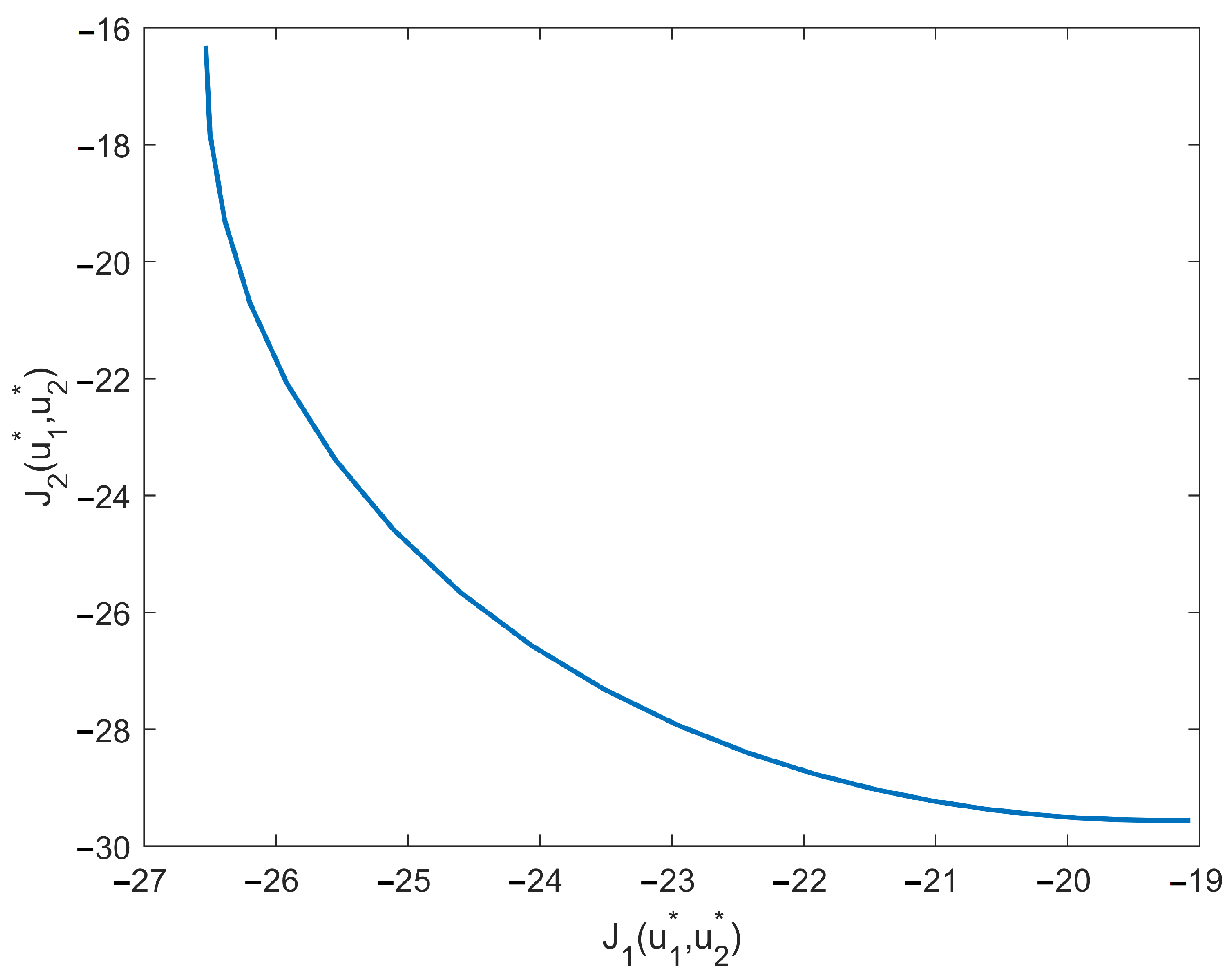
Remark 4.

Theorem 2 shows how to obtain the value of $J_i(u^{*},v^{*},x_0),i=1,2,\dots ,N$ for any controllers $u_i^{*}$. According to the definition of Pareto solutions, $J_i(u^{*},v^{*},x_0)$ is not uniquely determined. When $\alpha \in \mathbb{A}$ changes, $J_i(u^{*},v^{*},x_0)$ will also change, and the set of all Pareto solutions constitutes the Pareto frontier.

Remark 5.

Because of the existence of ${\tilde{\mathcal{A}}}_k$, ${\tilde{\mathcal{D}}}_k$, ${\widehat{\mathcal{A}}}_k$ and ${\widehat{\mathcal{D}}}_k$ in Equations (21) and (23), ${\mathcal{K}}_{\gamma }^k$ and ${\mathcal{K}}_p^k$ are coupled. To avoid overly complex solutions, the system (1) is reduced to a system with only state-dependent noise:

$$\left\{\begin{array}{c}{x}_{k+1}={\mathcal{A}}_k{x}_k+\sum _{i=1}^N{\mathcal{B}}_{i,k}{u}_{i,k}+{\mathcal{C}}_k{v}_k+{\mathcal{D}}_k{x}_k{w}_k,\hfill \\ z_k=\left[\begin{array}{c}{\mathcal{W}}_k{x}_k\\ {\mathcal{G}}_k{u}_k\end{array}\right],x_0\in {\mathcal{R}}^n,k\in {\mathcal{N}}_T.\hfill \end{array}\right.$$

(34)

Equations (21) and (23) can be rewritten as the follwing two coupled equations:

$${\mathcal{K}}_{\gamma }^k=-{\left({\gamma }^2{\mathcal{I}}_l+{\mathcal{C}}_k^{\prime }{\mathcal{P}}_v^{k+1}{\mathcal{C}}_k\right)}^{-1}{\mathcal{C}}_k^{\prime }{\left({\mathcal{P}}_v^{k+1}\right)}^{\prime }\left({\mathcal{A}}_k+{\mathcal{B}}_k{\mathcal{K}}_p^k\right),$$

(35)

$${\mathcal{K}}_p^k=-{\left({\mathcal{R}}_{\alpha }+{\mathcal{B}}_k^{\prime }{\mathcal{P}}_u^{k+1}{\mathcal{B}}_k\right)}^{†}{\mathcal{B}}_k^{\prime }{\mathcal{P}}_u^{k+1}\left({\mathcal{A}}_k+{\mathcal{C}}_k{\mathcal{K}}_{\gamma }^k\right).$$

(36)

Substituting $K_p^k$ into the Equation (35), after calculations, ${\mathcal{K}}_{\gamma }^k$ is as follows:

$$\begin{array}{cc}\hfill {\mathcal{K}}_{\gamma }^k=& \left[{({\gamma }^2{\mathcal{I}}_l+{\mathcal{C}}_k^{\prime }{\mathcal{P}}_v^{k+1}{\mathcal{C}}_k)}^{-1}{\mathcal{C}}_k^{\prime }{\left({\mathcal{P}}_v^{k+1}\right)}^{\prime }{\mathcal{B}}_k{({\mathcal{R}}_{\alpha }+{\mathcal{B}}_k^{\prime }{\mathcal{P}}_u^{k+1}{\mathcal{B}}_k)}^{†}{\mathcal{B}}_k^{\prime }{\mathcal{P}}_u^{k+1}{\mathcal{C}}_k-{\mathcal{I}}_l\right]\hfill \\ \hfill & \times {({\gamma }^2{\mathcal{I}}_l+{\mathcal{C}}_k^{\prime }{\mathcal{P}}_v^{k+1}{\mathcal{C}}_k)}^{-1}\left[{\mathcal{C}}_k^{\prime }{\left({\mathcal{P}}_v^{k+1}\right)}^{\prime }{\mathcal{A}}_k-{\mathcal{C}}_k^{\prime }{\left({\mathcal{P}}_v^{k+1}\right)}^{\prime }{\mathcal{B}}_k{({\mathcal{R}}_{\alpha }+{\mathcal{B}}_k{\mathcal{P}}_u^{k+1}{\mathcal{B}}_k)}^{†}{\mathcal{B}}_k^{\prime }{\mathcal{P}}_u^{k+1}{\mathcal{A}}_k\right].\hfill \end{array}$$

(37)

4. Example

In this section, we give a numerical example to show more details of calculating the Pareto optimal control with $H_{\infty }$ constraints.

Example 1.

Consider system (34) with $\mathcal{N}=2$, and the corresponding coefficients are given in

Table 1. Coefficients of dynamic system (34).

${\mathcal{A}}_{\mathit{k}}$	${\mathcal{B}}_{1,\mathit{k}}$	${\mathcal{B}}_{2,\mathit{k}}$	${\mathcal{C}}_{\mathit{k}}$	${\mathcal{D}}_{\mathit{k}}$	${\mathcal{W}}_{\mathit{k}}$	${\mathcal{G}}_{\mathit{k}}$
$\left[\begin{array}{cc}-1.2& 0\\ 0& 0.2\end{array}\right]$	$\left[\begin{array}{c}1.8\\ 1.1\end{array}\right]$	$\left[\begin{array}{c}1.5\\ 0.53\end{array}\right]$	$\left[\begin{array}{c}-0.05\\ -0.2\end{array}\right]$	$\left[\begin{array}{cc}-0.2& 0.5cos k\\ 0& 0.4tanh k\end{array}\right]$	$\left[\begin{array}{cc}-0.5& 0\\ 0& -0.5\end{array}\right]$	$\left[\begin{array}{cc}1.6& 0\\ 0& 0.4\end{array}\right]$

. The cost functionals of two players are

$$\begin{array}{c}\hfill {\mathcal{J}}_i=\sum _{k=0}^T\mathbb{E}\left(-0.5x_k^{\prime }{x}_k+2u_{i,k}^{\prime }{u}_{i,k}\right),i=1,2.\end{array}$$

The corresponding weighted sum cost functional is

$$\begin{array}{c}\hfill {\mathcal{J}}_{\alpha }(u,v,x_0)=\sum _{k=0}^T\mathbb{E}\left[-0.5x_k^{\prime }{x}_k+u_k^{\prime }\left[\begin{array}{cc}2{\alpha }_1& 0\\ 0& 2(1-{\alpha }_1)\end{array}\right]u_k\right].\end{array}$$

And the the robust cost functional ${\mathcal{J}}_v\left(u,v,x_0\right)$ is given as (13). Set the initial temperature $x_0={[-2-3]}^{\prime }$, ${\alpha }_1=0.8$, the disturbance attenuation $\gamma =0.8$, T = 10, $\mathcal{S}=I.$

The first step to get the solution of this Pareto game is to calculate ${\mathcal{K}}_{\gamma }^{10}$ and ${\mathcal{K}}_p^{10}$ by solving Equations (37) and (36) with ${\mathcal{P}}_v^{11}=0$ and ${\mathcal{P}}_u^{11}=0$. Then by solving the Equations (20) and (22), we get ${\mathcal{P}}_v^{10}$ and ${\mathcal{P}}_u^{10}$. Calculate like this until k=0, we get evolutions of ${\mathcal{P}}_v^k=\left[\begin{array}{cc}{\mathcal{P}}_{v11}& {\mathcal{P}}_{v12}\\ {\mathcal{P}}_{v12}& {\mathcal{P}}_{v22}\end{array}\right],$${\mathcal{P}}_u^k=\left[\begin{array}{cc}{\mathcal{P}}_{u11}& {\mathcal{P}}_{u12}\\ {\mathcal{P}}_{u12}& {\mathcal{P}}_{u22}\end{array}\right],$${\mathcal{K}}_{\gamma }^k$ and ${\mathcal{K}}_p^k$ shown in Figure 1 and Figure 2, respectively, which show the convergence of the solutions of coupled GDREs (20)–(23). From Figure 3 and Figure 4, we can konw that the constraints ${\mathcal{P}}_v^k\le 0$ and ${\mathcal{P}}_v^0+{\gamma }^2\mathcal{S}>0$ are satisfied, which means that the obtained ${\mathcal{P}}_v^k$ and ${\mathcal{P}}_u^k$ are valid.

According to the obtained ${\mathcal{K}}_{\gamma }^k$ and ${\mathcal{K}}_p^k$, we can get the Pareto efficient strategy $u_k^{*}={\mathcal{K}}_p^k{x}_k$ under the worst-case disturbance $v_k^{*}={\mathcal{K}}_{\gamma }^k{x}_k$ and the corresponding $x_k^{*}$, as shown in Figure 5 and Figure 6. It can be seen from Figure 6 that the system state is stable after $k=5$. Therefore, the control input $u_k^{*}$ obtained by Theorem 1 can achieve rapid convergence of the system state, even when external disturbance exists. Next, let $v=\overline{v}=0.8^{k}sin\left(k\right)$, we get the corresponding values of ${\sum }_{k=0}^{10}\mathbb{E}\left({\overline{z}}_k^{\prime }{\overline{z}}_k\right)$ and ${\sum }_{k=0}^{10}\mathbb{E}\left({\gamma }^2{\overline{v}}_k^{\prime }{\overline{v}}_k\right)+{\gamma }^2{x}_0^{\prime }\mathcal{S}{x}_0$ as shown in Figure 7. As a comparison, we apply the same disturbance to the algorithm without considering the $H_{\infty }$ constraint in [25], and obtain the corresponding ${\sum }_{k=0}^{10}\mathbb{E}\left({\widehat{z}}_k^{\prime }{\widehat{z}}_k\right)$ as shown by the dotted line in Figure 7. Obviously, for the same disturbance, the system output under the control input obtained in this paper has a smaller sum, and is less affected by the disturbance. In Figure 7, ${\sum }_{k=0}^{10}\mathbb{E}\left({\overline{z}}_k^{\prime }{\overline{z}}_k\right)$ is always smaller than ${\sum }_{k=0}^{10}\mathbb{E}\left({\gamma }^2{\overline{v}}_k^{\prime }{\overline{v}}_k\right)+{\gamma }^2{x}_0^{\prime }\mathcal{S}{x}_0$, which demonstrates $∥{\mathcal{L}}_T∥<\gamma$, that is, the influence of disturbance on the system output is controlled within the set range. According to Definition 2, we can say that $u^{*}$ satisfies the $H_{\infty }$ constraint. Finally, let α vary on [0, 1]. By solving Equation (31), we can get different Pareto solutions, which constitutes the Pareto frontier as shown in Figure 8. It can be seen from Figure 8 that on the Pareto front if $J_1(u_1^{*},u_2^{*},v^{*},x_0)$ gets better $J_2(u_1^{*},u_2^{*},v^{*},x_0)$ will get worse, as every set of solutions on the Pareto frontier satisfies Definition 1. It also shows that the methods proposed in this paper are effective in obtaining Pareto solutions and Pareto frontier. Each of the Pareto solutions on the Pareto frontier satisfies that it cannot be improved by all the players simultaneously. Therefore, we can make tradeoffs on the Pareto frontier to determine desired $J_1(u_1^{*},u_2^{*},v^{*},x_0)$ and $J_2(u_1^{*},u_2^{*},v^{*},x_0)$.

5. Conclusions

This paper has studied the Pareto optimal strategy under $H_{\infty }$ constraint for finite horizon discrete-time stochastic systems, where the SBRL with nonzero initial value has been obtained. By means of four coupled GDREs, the necessary and sufficient conditions for the existence of Pareto optimal strategy under worst-case disturbance have been given. The Pareto solutions of each player corresponding to the optimal strategy have been studied. Simulation results of a numerical example have shown the effectiveness of the main results. In the future, we can extend the obtained Pareto optimal strategy under $H_{\infty }$ constraint to the infinite horizon case [13] or apply it to the mean-field stochastic system [23] and time-delay system [33]. We can also explore model-free Pareto optimal control under $H_{\infty }$ constraint through reinforcement learning methods [34].

References

1. Cui, Y.; Geng, Z.; Zhu, Q.; Han, Y. Review: Multi-objective optimization methods and application in energy saving. Energy 2017, 125, 681–704. [Google Scholar] [CrossRef]
2. Basar, T.; Olsder, G.J. Dynamic Noncooperative Game Theory, 2nd ed.; SIAM: Philadelphia, PA, USA, 1999. [Google Scholar]
3. Yeung, D.W.K.; Petrosyan, L.A. Cooperative Stochastic Differential Games; Springer: New York, NY, USA, 2006. [Google Scholar]
4. Gromova, E.V.; Petrosyan, L.A. On an approach to constructing a characteristic function in cooperative differential games. Autom. Remote Control 2017, 78, 1680–1692. [Google Scholar] [CrossRef]
5. Mukaidani, H.; Xu, H. Robust SOF Stackelberg game for stochastic LPV systems. Sci. China Inf. Sci. 2021, 64, 200202. [Google Scholar] [CrossRef]
6. Acemoglu, D. Introduction to economic growth. J. Econ. Theory 2012, 147, 545–550. [Google Scholar] [CrossRef]
7. Dockner, E.J.; Jorgensen, S.; Van Long, N.; Sorger, G. Differential Games in Economics and Management Science; Cambridge University Press: Cambridge, UK, 2000. [Google Scholar]
8. Lavin, A. A Pareto front-based multiobjective path planning algorithm. arXiv 2015, arXiv:1505.05947. [Google Scholar]
9. Hou, Y.; Wu, N.; Zhou, M.; Li, Z. Pareto-optimization for scheduling of crude oil operations in refinery via genetic algorithm. IEEE Trans. Syst. Man Cybern. Syst. 2015, 47, 517–530. [Google Scholar] [CrossRef]
10. Wang, S.; Zhao, Y.; Xu, J.; Yuan, J.; Hsu, C.H. Edge server placement in mobile edge computing. J. Parallel Distrib. Comput. 2019, 127, 160–168. [Google Scholar] [CrossRef]
11. Engwerda, J.C. Linear-Quadratic Dynamic Optimization and Differential Games; Wiley: Chichester, UK, 2005. [Google Scholar]
12. Engwerda, J.C. The regular convex cooperative linear quadratic control problem. Automatica 2008, 44, 2453–2457. [Google Scholar] [CrossRef]
13. Reddy, P.V.; Engwerda, J.C. Pareto optimality in infinite horizon linear quadratic differential games. Automatica 2013, 49, 1705–1714. [Google Scholar] [CrossRef]
14. Lin, Y.; Jiang, X.; Zhang, W. Necessary and sufficient conditions for Pareto optimality of the stochastic systems in finite horizon. Automatica 2018, 94, 341–348. [Google Scholar] [CrossRef]
15. Zhu, H.; Zhang, C. Finite horizon linear quadratic dynamic games for discrete-time stochastic systems with N-players. Oper. Res. Lett. 2016, 44, 307–312. [Google Scholar] [CrossRef]
16. Peng, C.; Zhang, W.; Ma, L. Infinite horizon multiobjective optimal control of stochastic cooperative linear-quadratic dynamic difference games. J. Frankl. Inst. 2021, 358, 8288–8307. [Google Scholar] [CrossRef]
17. Peng, C.; Zhang, W. Multiobjective dynamic optimization of cooperative difference games in infinite horizon. IEEE Trans. Syst. Man, Cybern. Syst. 2021, 51, 6669–6680. [Google Scholar] [CrossRef]
18. Ahmed, M.; Mukaidani, H.; Shima, T. H constraint Pareto optimal strategy for stochastic LPV systems. Int. Game Theory Rev. 2018, 20, 1750031. [Google Scholar] [CrossRef] [Green Version]
19. Jiang, X.; Tian, S.; Zhang, T.; Zhang, W. Pareto optimal strategy for linear stochastic systems with H constraint in finite horizon. Inf. Sci. 2020, 512, 1103–1117. [Google Scholar] [CrossRef]
20. Wonham, W.M. On a matrix Riccati equation of stochastic control. SIAM J. Control 1968, 6, 681–697. [Google Scholar] [CrossRef]
21. Li, Z.; Fu, M.; Zhang, H.; Wu, Z. Mean field stochastic linear quadratic games for continuum-parameterized multi-agent systems. J. Frankl. Inst. 2018, 355, 5240–5255. [Google Scholar] [CrossRef]
22. Iourtchenko, D.V. Solution to a class of stochastic LQ problems with bounded control. Automatica 2009, 45, 1439–1442. [Google Scholar] [CrossRef]
23. Zhang, W.; Peng, C. Indefinite mean-field stochastic cooperative linear-quadratic dynamic difference game with its application to the network security model. IEEE Trans. Cybern. 2021, 1–14. [Google Scholar] [CrossRef]
24. Chen, S.; Li, X.; Zhou, X. Stochastic linear quadratic regulators with indefinite control weight costs. SIAM J. Control Optim. 1998, 36, 1685–1702. [Google Scholar] [CrossRef]
25. Ait Rami, M.; Chen, X.; Zhou, X. Discrete-time indefinite LQ control with state and control dependent noises. J. Glob. Optim. 2002, 23, 245–265. [Google Scholar] [CrossRef]
26. Limebeer, D.J.N.; Anderson, B.D.O.; Hendel, B. A Nash game approach to mixed H2/H control. IEEE Trans. Autom. Control 1994, 39, 69–82. [Google Scholar] [CrossRef]
27. Zhang, W.; Xie, L.; Chen, B. Stochastic H2/H Control: A Nash Game Approach; CRC Press: Boca Raton, FL, USA, 2017. [Google Scholar]
28. Zhang, T.; Deng, F.; Sun, Y.; Shi, P. Fault estimation and fault-tolerant control for linear discrete time-varying stochastic systems. Sci. China Inf. Sci. 2021, 64, 200201. [Google Scholar] [CrossRef]
29. Jiang, X.; Tian, S.; Zhang, W. pth moment exponential stability of general nonlinear discrete-time stochastic systems. Sci. China Inf. Sci. 2021, 64, 209204. [Google Scholar] [CrossRef]
30. Leitmann, G. Cooperative and Noncooperative Many Player Differential Games; Springer: New York, NY, USA, 1974. [Google Scholar]
31. Zhang, W.; Huang, Y.; Zhang, H. Stochastic H2/H control for discrete-time systems with state and disturbance dependent noise. Automatica 2007, 43, 513–521. [Google Scholar] [CrossRef]
32. Ait Rami, M.; Moore, J.B.; Zhou, X. Indefinite stochastic linear quadratic control and generalized differential Riccati equation. SIAM J. Control Optim. 2001, 40, 1296–1311. [Google Scholar] [CrossRef] [Green Version]
33. Yan, H.; Zhou, X.; Zhang, H.; Yang, F.; Wu, Z. A novel sliding mode estimation for microgrid control with communication time delays. IEEE Trans. Smart Grid 2019, 10, 1509–1520. [Google Scholar] [CrossRef]
34. Kiumarsi, B.; Lewis, F.L.; Modares, H.; Karimpour, A.; Bagher, M.; Sistani, N. Reinforcement Q-learning for optimal tracking control of linear discrete-time systems with unknown dynamics. Automatica 2014, 50, 1167–1175. [Google Scholar] [CrossRef]
Figure 1. Convergence of P v k and P u k .
Processes 10 01344 g001
Figure 2. Convergence of K γ k and K p k .
Processes 10 01344 g002
Figure 3. The maximum eigenvalue of P v k .
Processes 10 01344 g003
Figure 4. The minimum eigenvalue of P v k + γ 2 S .
Processes 10 01344 g004
Figure 5. Pareto optimal strategies u 1 , k * and u 2 , k * .
Processes 10 01344 g005
Figure 6. Optimal state x k * .
Processes 10 01344 g006
Figure 7. H performance analysis with v = 0 . 8 k s i n ( k ) .
Processes 10 01344 g007
Figure 8. Pareto frontier.
Processes 10 01344 g008