
Critical Procedure Identification Method Considering the Key Quality Characteristics of the Product Manufacturing Process


Abstract
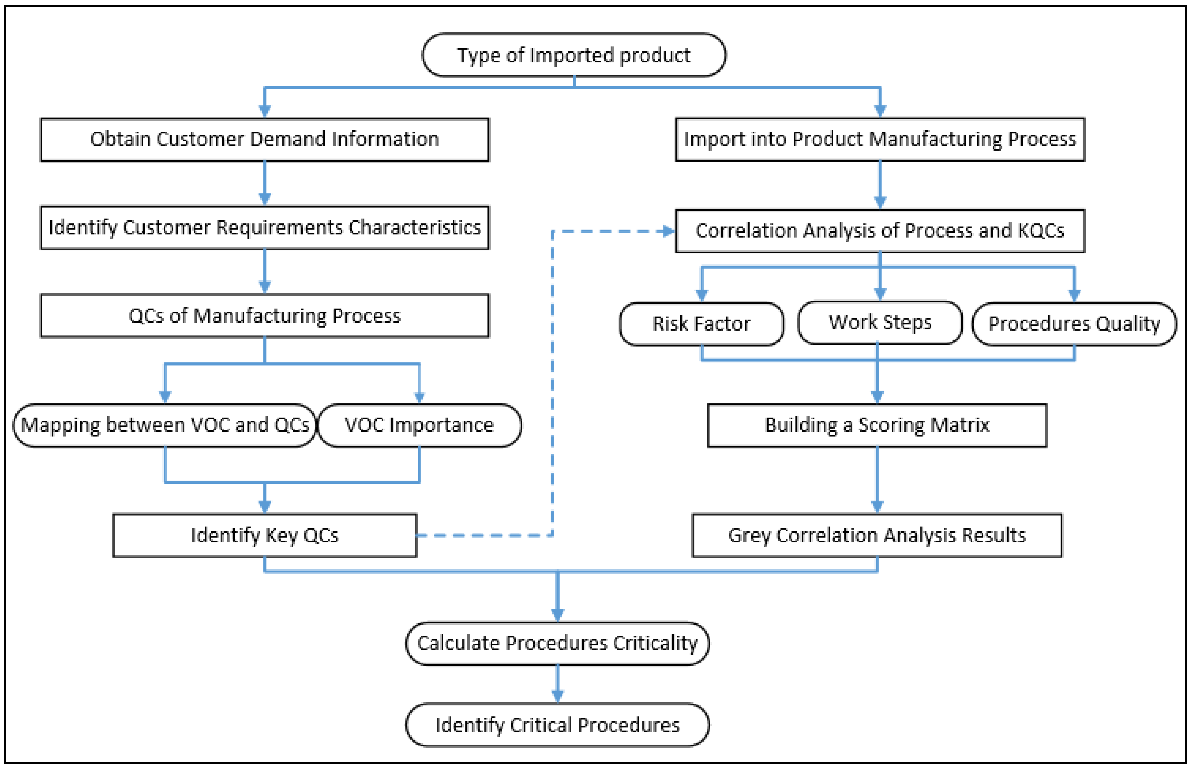
:1. Introduction
2. Obtain KQCs with Genetic BP Neural Network
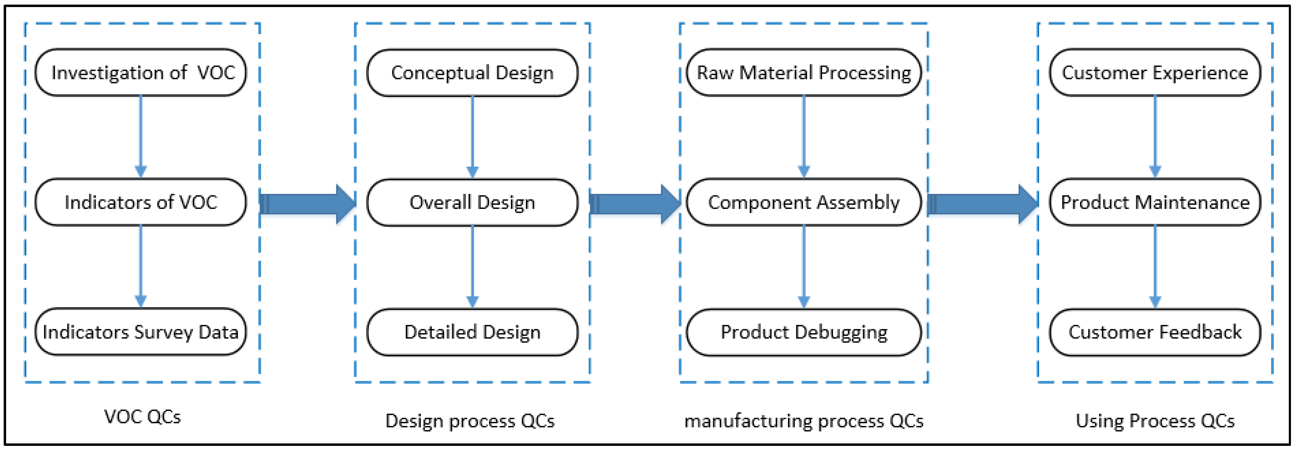
2.1. Mapping Process of Product QCs
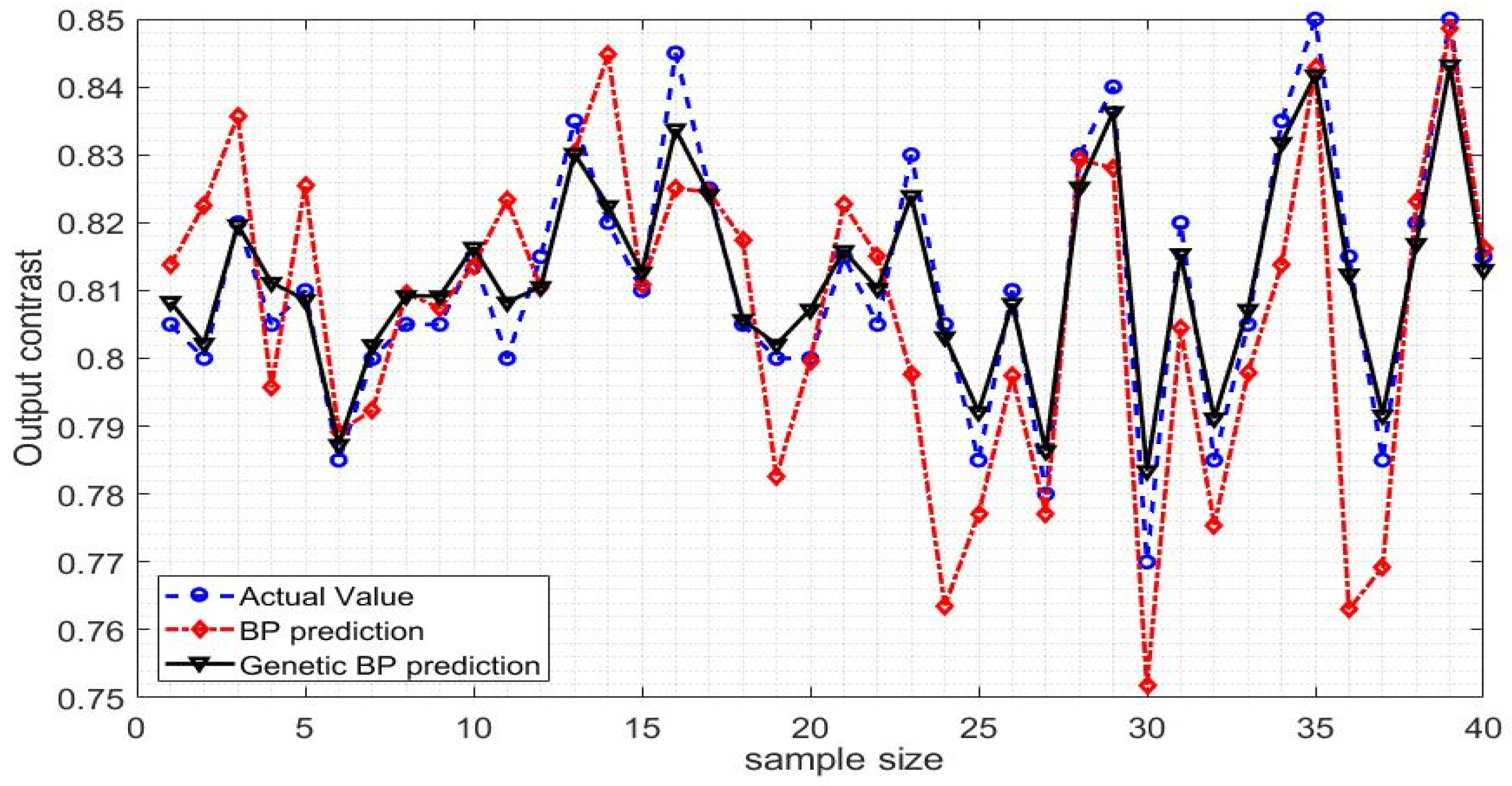
2.2. The Genetic BP Neural Network Theory
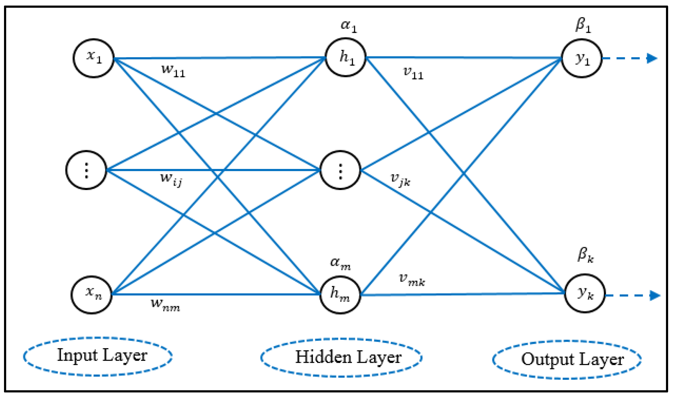
2.2.1. BP Neural Network
2.2.2. Design of Genetic BP Neural Network
- Set up BP neural network: Two main parameters (weight and threshold) of the BP neural network are adjusted by a genetic algorithm. The hidden layer activation function is set as an S-type transfer function, as shown in the equation , the output layer activation function is set to a linear transport function, as shown in the equation , and take the mean square error as the loss function, as shown in the equation .
- Initial population: The weights and thresholds of the BP neural network are encoded by actual number coding. The population size is 80 and the evolutionary generation is 100 generations.
- Fitness function of a genetic algorithm: Genetic algorithm takes the individual with the most prominent fitness value as the optimal individual. Therefore, the reciprocal of the mean square error is selected as the fitness function, as shown in Equation (1).
- Genetic operators: Use the most common genetic operators, namely roulette selection, simulated binary crossover, and polynomial mutation operators, using an elite retention strategy. Set crossover probability to 0.8 and mutation probability to 0.1.
2.3. KQCs in the Product Manufacturing Process
2.3.1. Calculate Customer Requirements Indicator’s Importance
2.3.2. Determination of Mapping Degree
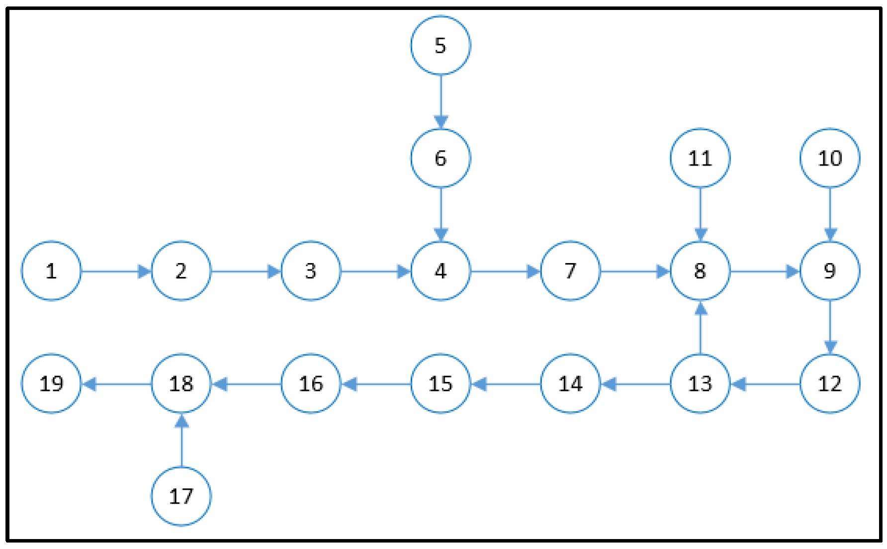
3. Identify Critical Procedure in the Manufacturing Process
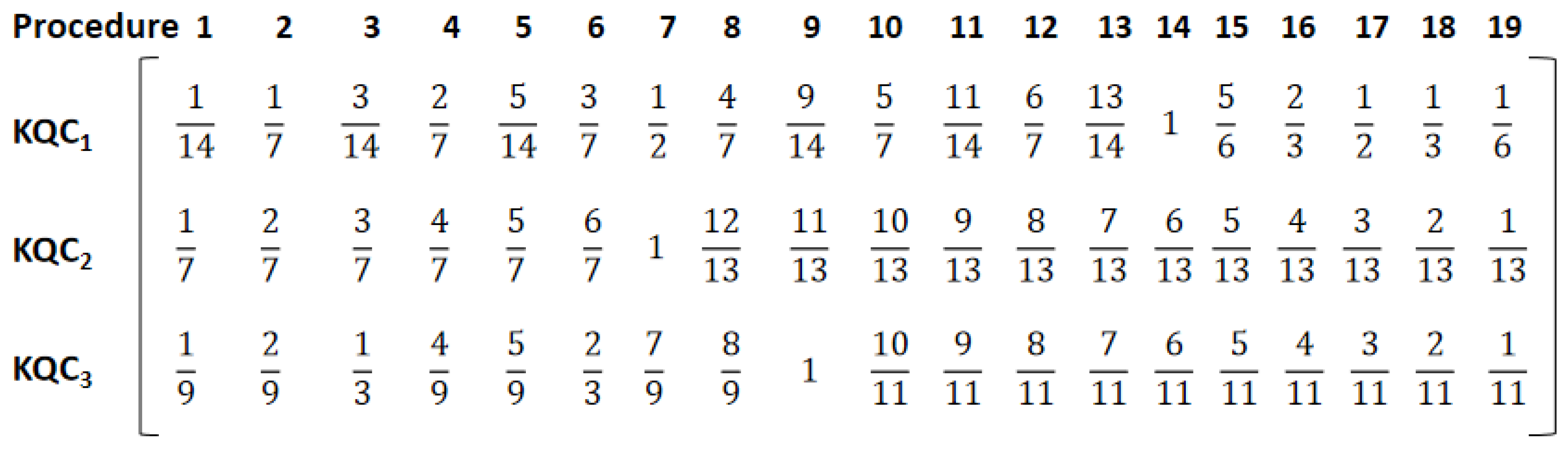
3.1. Determine the Correlation Degree Scoring Matrix
3.2. Grey Correlation Degree Calculation
3.2.1. Determine the Analysis Sequence
3.2.2. Dimensionless Processing of Data
3.2.3. Calculated Correlation Degree
3.3. Calculated Procedures Criticality
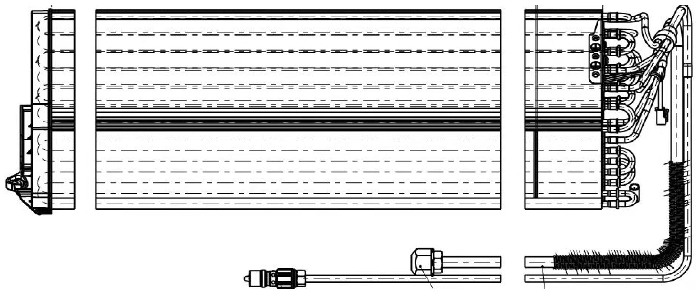
4. Case Study
4.1. Obtaining KQCs and Their Importance
4.2. Grey Relational Analysis Identifies Key Procedure
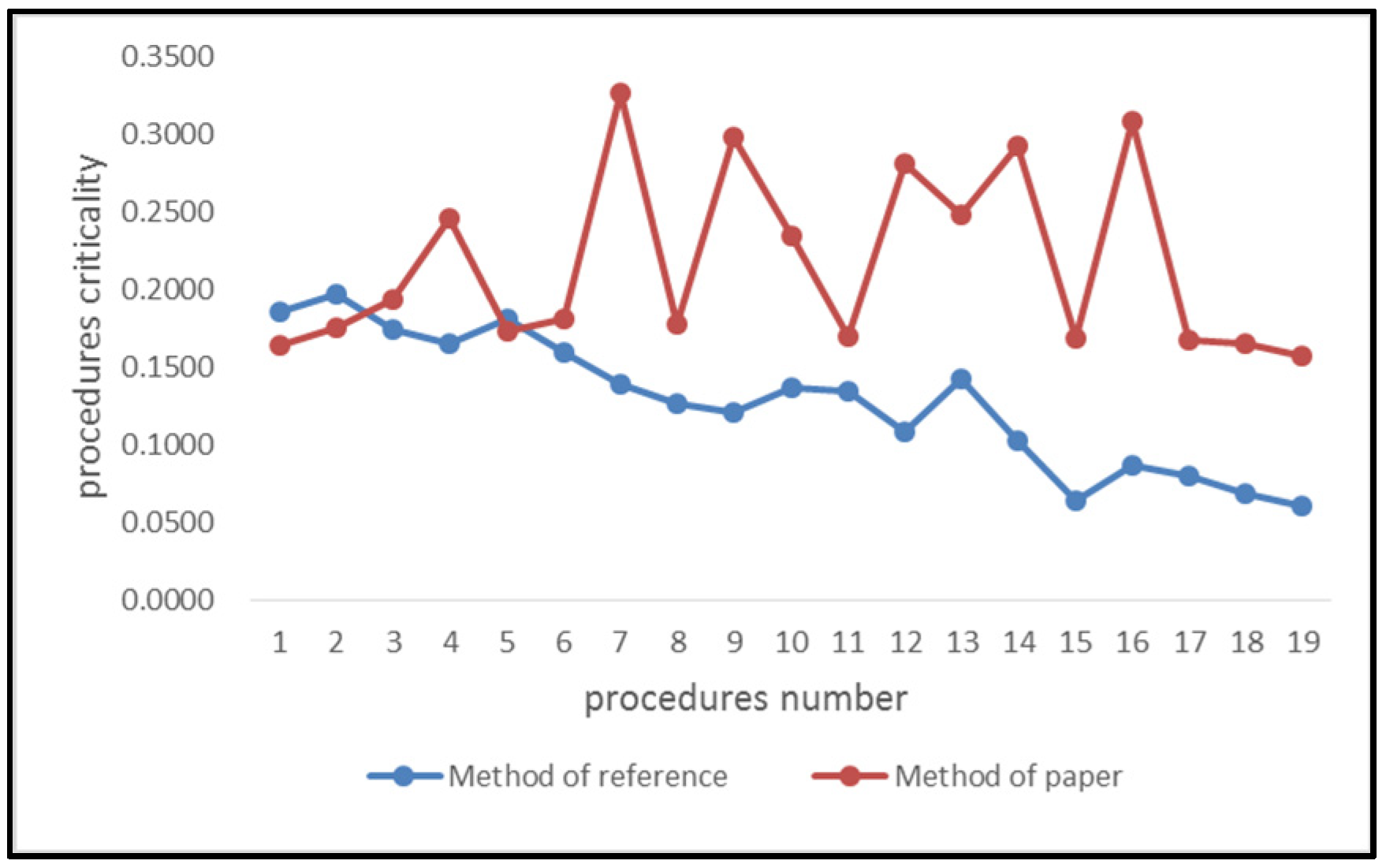
4.3. Comparison Study
5. Conclusions
Author Contributions
Funding
Data Availability Statement
Acknowledgments
Conflicts of Interest
Appendix A

| Evaluation Value | QC1 | QC2 | QC3 | QC4 | QC5 | QC6 | QC7 | QC8 | QC9 | QC10 | QC11 | QC12 |
|---|---|---|---|---|---|---|---|---|---|---|---|---|
| Sample: 1 | 0.081 | 0.047 | 0.033 | 0.031 | 0.180 | 0.048 | 0.106 | 0.157 | 0.210 | 0.025 | 0.062 | 0.023 |
| 2 | 0.091 | 0.033 | 0.023 | 0.031 | 0.151 | 0.047 | 0.131 | 0.214 | 0.125 | 0.030 | 0.060 | 0.066 |
| 3 | 0.087 | 0.039 | 0.023 | 0.037 | 0.160 | 0.049 | 0.104 | 0.217 | 0.158 | 0.036 | 0.065 | 0.026 |
| 4 | 0.091 | 0.040 | 0.026 | 0.029 | 0.150 | 0.046 | 0.116 | 0.163 | 0.214 | 0.024 | 0.064 | 0.038 |
| 5 | 0.039 | 0.020 | 0.027 | 0.060 | 0.153 | 0.064 | 0.198 | 0.104 | 0.188 | 0.040 | 0.086 | 0.022 |
| 6 | 0.038 | 0.022 | 0.032 | 0.053 | 0.155 | 0.064 | 0.200 | 0.101 | 0.183 | 0.042 | 0.086 | 0.024 |
| 7 | 0.037 | 0.021 | 0.032 | 0.057 | 0.137 | 0.068 | 0.209 | 0.112 | 0.179 | 0.041 | 0.085 | 0.023 |
| 8 | 0.030 | 0.042 | 0.022 | 0.054 | 0.089 | 0.101 | 0.165 | 0.198 | 0.171 | 0.046 | 0.065 | 0.017 |
| 9 | 0.030 | 0.042 | 0.025 | 0.054 | 0.090 | 0.103 | 0.148 | 0.202 | 0.176 | 0.048 | 0.068 | 0.016 |
| 10 | 0.030 | 0.042 | 0.024 | 0.051 | 0.090 | 0.112 | 0.140 | 0.219 | 0.164 | 0.047 | 0.065 | 0.017 |
| 11 | 0.031 | 0.038 | 0.021 | 0.051 | 0.096 | 0.105 | 0.140 | 0.215 | 0.166 | 0.046 | 0.076 | 0.017 |
| 12 | 0.038 | 0.034 | 0.022 | 0.057 | 0.096 | 0.115 | 0.131 | 0.210 | 0.155 | 0.052 | 0.072 | 0.018 |
| 13 | 0.033 | 0.043 | 0.021 | 0.053 | 0.101 | 0.100 | 0.148 | 0.201 | 0.155 | 0.052 | 0.074 | 0.019 |
| 14 | 0.091 | 0.044 | 0.022 | 0.025 | 0.158 | 0.053 | 0.117 | 0.159 | 0.209 | 0.027 | 0.061 | 0.034 |
| 15 | 0.077 | 0.043 | 0.022 | 0.028 | 0.161 | 0.050 | 0.125 | 0.159 | 0.210 | 0.027 | 0.061 | 0.038 |
| 16 | 0.078 | 0.043 | 0.021 | 0.027 | 0.159 | 0.053 | 0.121 | 0.155 | 0.220 | 0.028 | 0.060 | 0.035 |
| 17 | 0.076 | 0.044 | 0.018 | 0.028 | 0.177 | 0.056 | 0.116 | 0.133 | 0.198 | 0.029 | 0.062 | 0.064 |
| 18 | 0.078 | 0.042 | 0.020 | 0.022 | 0.179 | 0.057 | 0.122 | 0.130 | 0.194 | 0.029 | 0.057 | 0.071 |
| 19 | 0.061 | 0.041 | 0.047 | 0.080 | 0.112 | 0.071 | 0.146 | 0.120 | 0.171 | 0.037 | 0.095 | 0.020 |
| 20 | 0.054 | 0.044 | 0.048 | 0.079 | 0.112 | 0.069 | 0.145 | 0.121 | 0.178 | 0.031 | 0.087 | 0.034 |
| 21 | 0.084 | 0.048 | 0.030 | 0.025 | 0.168 | 0.060 | 0.106 | 0.196 | 0.158 | 0.025 | 0.068 | 0.034 |
| 22 | 0.068 | 0.041 | 0.029 | 0.030 | 0.170 | 0.066 | 0.116 | 0.178 | 0.173 | 0.025 | 0.077 | 0.028 |
| 23 | 0.065 | 0.047 | 0.031 | 0.024 | 0.169 | 0.063 | 0.112 | 0.178 | 0.183 | 0.024 | 0.075 | 0.029 |
| 24 | 0.061 | 0.046 | 0.031 | 0.024 | 0.177 | 0.064 | 0.111 | 0.179 | 0.176 | 0.025 | 0.075 | 0.032 |
| 25 | 0.075 | 0.044 | 0.027 | 0.028 | 0.170 | 0.063 | 0.100 | 0.183 | 0.171 | 0.025 | 0.077 | 0.038 |
| 26 | 0.030 | 0.039 | 0.022 | 0.065 | 0.074 | 0.091 | 0.167 | 0.159 | 0.200 | 0.048 | 0.084 | 0.023 |
| 27 | 0.038 | 0.037 | 0.021 | 0.066 | 0.072 | 0.086 | 0.166 | 0.159 | 0.205 | 0.042 | 0.080 | 0.029 |
| 28 | 0.043 | 0.026 | 0.019 | 0.053 | 0.076 | 0.085 | 0.163 | 0.169 | 0.204 | 0.045 | 0.084 | 0.033 |
| 29 | 0.051 | 0.031 | 0.019 | 0.060 | 0.069 | 0.096 | 0.154 | 0.160 | 0.209 | 0.049 | 0.079 | 0.025 |
| 30 | 0.043 | 0.028 | 0.025 | 0.056 | 0.057 | 0.101 | 0.149 | 0.172 | 0.218 | 0.055 | 0.064 | 0.034 |
| 31 | 0.043 | 0.021 | 0.024 | 0.067 | 0.181 | 0.060 | 0.146 | 0.115 | 0.150 | 0.044 | 0.124 | 0.025 |
| 32 | 0.039 | 0.025 | 0.019 | 0.060 | 0.147 | 0.062 | 0.146 | 0.122 | 0.163 | 0.046 | 0.152 | 0.021 |
| 33 | 0.038 | 0.019 | 0.021 | 0.059 | 0.165 | 0.063 | 0.133 | 0.141 | 0.156 | 0.045 | 0.135 | 0.026 |
| 34 | 0.039 | 0.023 | 0.019 | 0.060 | 0.155 | 0.066 | 0.142 | 0.149 | 0.153 | 0.043 | 0.117 | 0.035 |
| 35 | 0.073 | 0.024 | 0.020 | 0.051 | 0.132 | 0.070 | 0.131 | 0.158 | 0.156 | 0.034 | 0.118 | 0.033 |
| 36 | 0.066 | 0.040 | 0.022 | 0.024 | 0.157 | 0.050 | 0.118 | 0.202 | 0.182 | 0.031 | 0.074 | 0.036 |
| 37 | 0.061 | 0.039 | 0.020 | 0.024 | 0.149 | 0.051 | 0.120 | 0.211 | 0.182 | 0.031 | 0.079 | 0.034 |
| 38 | 0.063 | 0.042 | 0.020 | 0.023 | 0.153 | 0.063 | 0.113 | 0.190 | 0.184 | 0.035 | 0.083 | 0.031 |
| 39 | 0.060 | 0.038 | 0.026 | 0.026 | 0.147 | 0.064 | 0.110 | 0.215 | 0.180 | 0.029 | 0.074 | 0.033 |
| 40 | 0.064 | 0.036 | 0.032 | 0.035 | 0.148 | 0.064 | 0.111 | 0.198 | 0.174 | 0.031 | 0.075 | 0.033 |
| Procedure Number | 1 | 2 | 3 | 4 | 5 | 6 | 7 | 8 | 9 | 10 | 11 | 12 | 13 | 14 | 15 | 16 | 17 | 18 | 19 |
|---|---|---|---|---|---|---|---|---|---|---|---|---|---|---|---|---|---|---|---|
| S | 6 | 6 | 4 | 4 | 3 | 3 | 5 | 3 | 4 | 5 | 3 | 4 | 4 | 4 | 6 | 4 | 6 | 5 | 5 |
| O | 5 | 5 | 5 | 7 | 4 | 4 | 4 | 2 | 4 | 5 | 3 | 5 | 5 | 3 | 5 | 5 | 6 | 3 | 2 |
| D | 6 | 4 | 5 | 5 | 2 | 5 | 6 | 4 | 7 | 6 | 4 | 6 | 5 | 4 | 6 | 3 | 7 | 6 | 5 |
| VOC Indicators Survey | VOC1 | VOC2 | VOC3 | VOC4 | VOC5 | VOC6 | VOC7 | VOC8 | VOC9 | VOC10 |
|---|---|---|---|---|---|---|---|---|---|---|
| Sample: 1 | 0.85 | 1.00 | 0.90 | 0.85 | 0.90 | 0.75 | 0.60 | 0.70 | 0.85 | 0.65 |
| 2 | 1.00 | 1.00 | 0.85 | 0.80 | 0.75 | 0.70 | 0.65 | 0.75 | 0.75 | 0.75 |
| 3 | 0.90 | 0.95 | 0.95 | 0.90 | 0.95 | 0.65 | 0.75 | 0.80 | 0.70 | 0.65 |
| 4 | 0.85 | 0.95 | 0.90 | 0.85 | 0.85 | 0.65 | 0.70 | 0.85 | 0.85 | 0.60 |
| 5 | 0.80 | 0.95 | 0.90 | 0.85 | 0.80 | 0.70 | 0.60 | 0.85 | 0.80 | 0.85 |
| 6 | 0.85 | 0.90 | 0.90 | 0.80 | 0.85 | 0.70 | 0.55 | 0.75 | 0.75 | 0.80 |
| 7 | 0.80 | 0.85 | 0.85 | 0.80 | 0.80 | 0.75 | 0.75 | 0.85 | 0.85 | 0.70 |
| 8 | 0.75 | 1.00 | 1.00 | 0.75 | 0.95 | 0.65 | 0.60 | 0.90 | 0.70 | 0.75 |
| 9 | 0.90 | 1.00 | 0.95 | 0.80 | 0.90 | 0.65 | 0.65 | 0.85 | 0.70 | 0.65 |
| 10 | 0.85 | 1.00 | 0.85 | 0.85 | 1.00 | 0.70 | 0.65 | 0.90 | 0.75 | 0.60 |
| 11 | 0.85 | 1.00 | 0.85 | 0.90 | 0.95 | 0.70 | 0.70 | 0.75 | 0.75 | 0.55 |
| 12 | 1.00 | 0.90 | 0.90 | 1.00 | 0.85 | 0.75 | 0.65 | 0.70 | 0.80 | 0.60 |
| 13 | 0.80 | 0.95 | 0.90 | 0.85 | 0.90 | 0.60 | 0.70 | 1.00 | 0.85 | 0.80 |
| 14 | 0.75 | 0.95 | 0.95 | 0.95 | 0.75 | 0.75 | 0.70 | 0.85 | 0.80 | 0.75 |
| 15 | 0.85 | 0.95 | 1.00 | 0.90 | 0.85 | 0.80 | 0.65 | 0.75 | 0.75 | 0.60 |
| 16 | 0.90 | 0.90 | 0.85 | 0.85 | 0.85 | 0.85 | 0.75 | 0.80 | 1.00 | 0.70 |
| 17 | 0.95 | 1.00 | 0.85 | 0.85 | 0.80 | 0.75 | 0.70 | 0.85 | 0.85 | 0.65 |
| 18 | 0.90 | 0.95 | 0.80 | 0.80 | 0.80 | 0.70 | 0.70 | 0.90 | 0.75 | 0.75 |
| 19 | 0.80 | 0.90 | 0.95 | 0.95 | 0.85 | 0.70 | 0.55 | 0.85 | 0.80 | 0.65 |
| 20 | 0.80 | 0.95 | 0.95 | 0.90 | 0.90 | 0.65 | 0.65 | 0.80 | 0.80 | 0.60 |
| 21 | 0.85 | 0.95 | 0.90 | 0.90 | 0.95 | 0.65 | 0.70 | 0.85 | 0.75 | 0.65 |
| 22 | 0.75 | 1.00 | 0.85 | 0.80 | 1.00 | 0.60 | 0.65 | 0.95 | 0.75 | 0.70 |
| 23 | 1.00 | 1.00 | 0.90 | 0.80 | 0.85 | 0.75 | 0.60 | 0.90 | 0.85 | 0.65 |
| 24 | 0.90 | 0.85 | 0.95 | 1.00 | 0.80 | 0.70 | 0.55 | 0.85 | 0.85 | 0.60 |
| 25 | 0.85 | 0.95 | 0.85 | 0.75 | 0.85 | 0.75 | 0.60 | 0.80 | 0.80 | 0.65 |
| 26 | 0.90 | 0.95 | 1.00 | 0.85 | 0.85 | 0.65 | 0.55 | 0.75 | 0.85 | 0.75 |
| 27 | 0.90 | 0.90 | 0.95 | 0.80 | 0.90 | 0.60 | 0.60 | 0.70 | 0.75 | 0.70 |
| 28 | 0.90 | 0.90 | 1.00 | 0.95 | 0.95 | 0.65 | 0.75 | 0.85 | 0.70 | 0.65 |
| 29 | 0.85 | 0.95 | 0.90 | 1.00 | 0.90 | 0.60 | 0.70 | 0.85 | 1.00 | 0.65 |
| 30 | 0.75 | 0.85 | 0.85 | 0.80 | 0.90 | 0.65 | 0.65 | 0.80 | 0.85 | 0.60 |
| 31 | 0.85 | 0.90 | 0.95 | 0.85 | 0.85 | 0.70 | 0.65 | 0.90 | 0.80 | 0.75 |
| 32 | 0.80 | 0.90 | 1.00 | 0.75 | 0.85 | 0.75 | 0.60 | 0.75 | 0.75 | 0.70 |
| 33 | 0.85 | 0.95 | 0.85 | 0.70 | 0.80 | 0.70 | 0.70 | 0.95 | 0.80 | 0.75 |
| 34 | 0.85 | 0.95 | 0.90 | 0.90 | 0.90 | 0.65 | 0.70 | 1.00 | 0.85 | 0.65 |
| 35 | 0.90 | 1.00 | 0.90 | 0.85 | 1.00 | 0.70 | 0.75 | 0.85 | 0.90 | 0.65 |
| 36 | 1.00 | 0.95 | 0.85 | 0.80 | 0.85 | 0.65 | 0.60 | 1.00 | 0.85 | 0.60 |
| 37 | 0.95 | 0.90 | 0.85 | 0.85 | 0.80 | 0.75 | 0.65 | 0.80 | 0.75 | 0.55 |
| 38 | 0.80 | 0.95 | 0.90 | 1.00 | 0.85 | 0.80 | 0.55 | 0.80 | 0.85 | 0.70 |
| 39 | 0.85 | 1.00 | 1.00 | 0.95 | 0.90 | 0.75 | 0.70 | 0.90 | 0.80 | 0.65 |
| 40 | 0.85 | 0.95 | 0.95 | 0.80 | 0.85 | 0.75 | 0.65 | 0.85 | 0.75 | 0.75 |
| Output: VOC comprehensive evaluation | 0.800 | 0.815 | 0.835 | 0.820 | 0.810 | 0.845 | 0.825 | 0.805 | 0.800 | 0.800 |
References
- Shuai, Q.; Yao, X. A hybrid genetic algorithm for flexible job-shop scheduling problem. Ind. Eng. J. 2013, 16, 31–37. [Google Scholar]
- Li, Y.; Zhang, F.; Yan, Y. Multi-Source uncertainty considered assembly process quality control based on surrogate model and information entropy. Struct. Multidiscip. Optim. 2019, 59, 1685–1701. [Google Scholar] [CrossRef]
- Mao, W.; Liu, P. Strengthen the quality control of bus production process. Bus Coach. Technol. Res. 2009, 31, 59–61. [Google Scholar]
- Chen, K. Research on Intelligent Quality Control Method of Multi-Variety and Small-Batch Manufacturing Process. Master’s Dissertation, Shenyang University of Technology, Shenyang, China, 2021. [Google Scholar]
- Tang, W.; Yu, J.; Li, Y.; Tang, S. Application of quantitative identification and decomposition methods for product key characteristics. Comput. Integr. Manuf. Syst. 2011, 17, 2383–2388. [Google Scholar]
- Gabriela, E.; Dan, L.; Feng, J. Systematic continuous improvement model for variation management of key characteristics running with low capability. Int. J. Prod. Res. 2018, 56, 2370–2387. [Google Scholar]
- Tiuc, D.; Draghici, G.; Parvu, A.; Enache, B. Consideration about the determination and control of the key characteristics as part of planning quality of the product development process. Appl. Mech. Mater. 2015, 809, 1269–1274. [Google Scholar] [CrossRef]
- Zhang, W.; Zhang, G.; Li, Y.; Shao, Y.; Ran, Y. Key engineering characteristics extraction technology based on QFD. IEEE Access 2019, 7, 75105–75112. [Google Scholar] [CrossRef]
- Liu, H. Important effect in quality chain by grading essentiality of product quality character. Electron. Qual. 2007, 01, 45–47. [Google Scholar]
- Zhong, X. Research and Application of Key Procedure Recognition and Quality Control in Multi-Specification and Small-Batch Production. Master’s Dissertation, Chongqing University, Chongqing, China, 2017. [Google Scholar]
- Wang, N.; Yan, N.; Xu, Y.; Yang, J. Identification of key quality characteristics in complex multi-process manufacturing process. Stat. Decis. 2021, 37, 177–180. [Google Scholar]
- Jin, C.; Ran, Y.; Wang, Z.; Zhang, G. Prioritization of key quality characteristics with the three-dimensional HoQ model-based interval-valued spherical fuzzy-ORESTE method. Eng. Appl. Artif. Intell. 2021, 104, 104271. [Google Scholar] [CrossRef]
- Ma, L.; Mao, J.; Fan, H. Key Quality Characteristics Identification Method for Mechanical Product. Procedia CIRP 2016, 56, 50–54. [Google Scholar] [CrossRef] [Green Version]
- Wang, H.; Liang, L.; Niu, Z.; He, Z. Identification of CTQs for complex products based on mutual information and improved gravitational search algorithm. Math. Probl. Eng. 2015, 6, 765985. [Google Scholar] [CrossRef]
- Whitney, D.E. The role of key characteristics in the design of mechanical assemblies. Assem. Autom. 2006, 26, 315–322. [Google Scholar] [CrossRef]
- Chakhunashvili, A.; Johansson, P.M.; Bergman, B.L.S. Variation mode and effect analysis. Qual. Reliab. Eng. 2009, 25, 167–179. [Google Scholar]
- Zhang, M. Research on Quality Control Technology of Key Procedure for Small Batch Trial Process. Master’s Dissertation, Hangzhou Dianzi University, Hangzhou, China, 2013. [Google Scholar]
- Zheng, Y.; Zhang, Q.; Ma, H.; Zhang, L. A research on the quality control of wind turbine hub assembly process based on improved taguchi method. Ind. Eng. J. 2019, 22, 37–43. [Google Scholar]
- Xu, H.; Lan, K.; Ma, Y.; Zheng, Y. Segmentation workshop key process identification method and application facing to accuracy. Ship Eng. 2020, 42, 141–146. [Google Scholar]
- Latchomy, P.; Khader, P.S.A. Reliable job execution with process failure recovery in computational grid. Int. J. Inf. Commun. Technol. 2015, 7, 607–631. [Google Scholar] [CrossRef]
- Yuan, Q.W.; Shun, J.; Yuan, Q.H.; Li, Z.; Yin, X. Key process and quality characteristic identification for manufacturing systems using dynamic weighting function and D-S evidence theory. Int. J. Perform. Eng. 2018, 14, 1651–1665. [Google Scholar] [CrossRef] [Green Version]
- Yuan, Y.; Wu, X.; He, L.; Wang, X.; Wu, Q. Research on personalized product configuration network based on data mining. Manuf. Autom. 2021, 43, 77–81. [Google Scholar]
- Quan, Z.; Zhao, L.; Xu, B.; Fan, S. Application research of improved AEWMAQ control chart for mass customization. Mach. Tool Hydraul. 2021, 49, 8–12. [Google Scholar]
- Aslam, M.; Arif, O.H. Testing of grouped product for the weibull distribution using neutrosophic statistics. Symmetry 2018, 10, 403. [Google Scholar] [CrossRef] [Green Version]
- Aslam, M.; Khan, N.; Khan, M.Z. Monitoring the variability in the process using neutrosophic statistical interval method. Symmetry 2018, 10, 562. [Google Scholar] [CrossRef] [Green Version]
- Aslam, M.; Bantan, R.; Khan, N. Design of a new attribute control chart under neutrosophic statistics. Fuzzy Syst. 2019, 21, 433–440. [Google Scholar] [CrossRef]
- Aslam, M. Attribute control chart using the repetitive sampling under neutrosophic system. IEEE Access 2019, 7, 15367–15374. [Google Scholar] [CrossRef]
- Aslam, M. Analyzing wind power data using analysis of means under neutrosophic statistics. Soft Comput. 2021, 25, 7087–7093. [Google Scholar] [CrossRef]
- He, Y.; Tang, X.; Wang, M. Quality data management model in product design. Comput. Integr. Manuf. Syst. 2006, 12, 1161–1166. [Google Scholar]
- Zhang, G.; Ji, F.; Ren, X.; Ge, H.; Zhang, S. Key quality characteristics extraction model of complicated mechanical and electrical products. J. Chongqing Univ. 2010, 33, 8–14. [Google Scholar]
- Nik, M.A.; Fayazbakhsh, K.; Pasini, D.; Lessard, L. A comparative study of metamodeling methods for the design optimization of variable stiffness composites. Compos. Struct. 2014, 107, 494–501. [Google Scholar]
- Lanzi, L.; Giavotto, V. Post-Buckling optimization of composite stiffened panels: Computations and experiments. Compos. Struct. 2006, 73, 208–220. [Google Scholar] [CrossRef]
- Sun, S.; Yang, W.; Hu, Z. Multi-Objective optimization of sheet metal forming based on dynamic genetic neural network and grey relativity. Comput. Integr. Manuf. Syst. 2020, 26, 3309–3407. [Google Scholar]
- Cai, R.; Cui, Y.; Xue, P. Research on the methods of determining the number of hidden nodes in three-layer BP neural network. Comput. Inf. Technol. 2017, 25, 29–33. [Google Scholar]
- Qian, K.; Hou, Z.; Sun, D. Sound quality estimation of electric vehicles based on GA-BP artificial neural networks. Appl. Sci. 2020, 10, 5567. [Google Scholar] [CrossRef]
- Chen, K.; Liu, W.; Jiang, X.; Xu, S.; Wang, Y.; Liu, A. A method of key process identification and cluster analysis in multi-variety and small-batch manufacturing process. Comput. Integr. Manuf. Syst. 2022, 28, 812–825. [Google Scholar]
- Xiao, C.; Liu, W.; Zheng, H.; Chen, P.; Wang, N. Improved risk evaluation method in FMEA based on information axiom. J. Nanchang Univ. 2013, 35, 363–368. [Google Scholar]
- Jiao, B.; Ye, M. Determination of hidden unit number in a BP neural network. J. Shanghai Dianji Univ. 2013, 16, 113–116. [Google Scholar]
- Zhang, Y.; Zuo, Y.; Liu, J.; Jiang, L. Application and comparison of GA-BP and BP neural network in medical research. Chin. J. Health Stat. 2018, 35, 239–241. [Google Scholar]
- Tang, R.; Wang, G.; Tang, W.; Jia, S. Key process identification method for workshop quality management. J. Zhejiang Univ. 2012, 46, 1937–1942. [Google Scholar]


| KQCs | KQC 1 | KQC 2 | Procedures Criticality | ||
|---|---|---|---|---|---|
| Importance Degree | |||||
| Procedure 1 | |||||
| Procedure 2 | |||||
| Procedure k |
| QC1 | QC2 | QC3 | QC4 | QC5 | QC6 | QC7 | QC8 | QC9 | QC10 | QC11 | QC12 | ||
|---|---|---|---|---|---|---|---|---|---|---|---|---|---|
| 1 | 0.068 | 0.076 | 0.035 | 0.162 | 0.045 | 0.404 | 0.154 | 0.144 | 0.256 | 0.139 | 0.143 | 0.111 | 0.127 |
| 2 | 0.101 | 0.025 | 0.178 | 0.361 | 0.106 | 0.174 | 0.145 | 0.280 | 0.594 | 0.188 | 0.053 | 0.130 | 0.298 |
| 3 | 0.091 | 0.041 | 0.060 | 0.163 | 0.086 | 0.425 | 0.164 | 0.106 | 0.220 | 0.105 | 0.044 | 0.131 | 0.077 |
| 4 | 0.128 | 0.131 | 0.053 | 0.045 | 0.015 | 0.006 | 0.081 | 0.013 | 0.057 | 0.035 | 0.124 | 0.029 | 0.031 |
| 5 | 0.081 | 0.169 | 0.042 | 0.007 | 0.289 | 0.477 | 0.022 | 0.229 | 0.150 | 0.147 | 0.096 | 0.116 | 0.241 |
| 6 | 0.086 | 0.064 | 0.017 | 0.096 | 0.178 | 0.283 | 0.128 | 0.026 | 0.041 | 0.136 | 0.061 | 0.043 | 0.045 |
| 7 | 0.106 | 0.017 | 0.000 | 0.148 | 0.032 | 0.134 | 0.086 | 0.097 | 0.076 | 0.098 | 0.030 | 0.017 | 0.183 |
| 8 | 0.124 | 0.064 | 0.057 | 0.243 | 0.159 | 0.284 | 0.066 | 0.084 | 0.201 | 0.042 | 0.062 | 0.218 | 0.159 |
| 9 | 0.128 | 0.051 | 0.177 | 0.027 | 0.108 | 0.173 | 0.048 | 0.091 | 0.211 | 0.115 | 0.165 | 0.098 | 0.000 |
| 10 | 0.087 | 0.022 | 0.049 | 0.162 | 0.155 | 0.236 | 0.030 | 0.189 | 0.245 | 0.098 | 0.080 | 0.000 | 0.258 |
| 0.045 | 0.049 | 0.096 | 0.077 | 0.165 | 0.061 | 0.082 | 0.138 | 0.072 | 0.060 | 0.062 | 0.092 |
| Serial Number | Name | Cause of Quality | Procedure Quality | Work Step Quantity | Risk Coefficient |
|---|---|---|---|---|---|
| 1 | Aluminum foil fin online | Large-scale rewinding | 21 | 3 | 0.364 |
| 2 | Fixed aluminum foil fin | Copper tube defects | 33 | 2 | 0.306 |
| 3 | Install left bracket | Copper tube defects | 26 | 3 | 0.274 |
| 4 | Fill nitrogen | No nitrogen | 27 | 3 | 0.347 |
| 5 | Copper tube plastic | Copper tube twisted | 24 | 2 | 0.157 |
| 6 | Insert copper tube | Not insert | 18 | 2 | 0.225 |
| 7 | Welding | Welding leakage or blocking | 18 | 4 | 0.306 |
| 8 | Welding inspection | Unchecked | 17 | 2 | 0.177 |
| 9 | Check for fluency | Unchecked | 20 | 3 | 0.321 |
| 10 | Secure hoods | Install the dislocation | 23 | 2 | 0.332 |
| 11 | Tie the line | Omit | 16 | 1 | 0.306 |
| 12 | Charge high-pressure test | Unchecked | 19 | 4 | 0.306 |
| 13 | Test it with helium | Unchecked | 26 | 3 | 0.274 |
| 14 | Refrigerant injection | Miss filling refrigerant | 27 | 4 | 0.257 |
| 15 | Install PTC | Large installation error | 12 | 3 | 0.199 |
| 16 | A hot-melt adhesive | Plastic wire drawing | 30 | 4 | 0.364 |
| 17 | Tie the insulation pipe | Omit | 26 | 1 | 0.438 |
| 18 | Install insulation pipe | Not up to requirements | 26 | 2 | 0.284 |
| 19 | Products offline | Damaged | 27 | 2 | 0.232 |
| KQC1 | KQC2 | KQC3 | Procedure Criticality | |
|---|---|---|---|---|
| Weighted Value | 0.0960 | 0.1650 | 0.1380 | |
| 1 | 0.3333 | 0.4228 | 0.4512 | 0.1640 |
| 2 | 0.3437 | 0.4580 | 0.4819 | 0.1751 |
| 3 | 0.3589 | 0.5163 | 0.5310 | 0.1929 |
| 4 | 0.3945 | 0.6971 | 0.6700 | 0.2454 |
| 5 | 0.3421 | 0.4522 | 0.4769 | 0.1733 |
| 6 | 0.3488 | 0.4766 | 0.4978 | 0.1808 |
| 7 | 0.4315 | 1.0000 | 0.8661 | 0.3259 |
| 8 | 0.3486 | 0.4547 | 0.4969 | 0.1771 |
| 9 | 0.4508 | 0.7055 | 1.0000 | 0.2977 |
| 10 | 0.4300 | 0.5719 | 0.7188 | 0.2348 |
| 11 | 0.3522 | 0.4243 | 0.4739 | 0.1692 |
| 12 | 0.5993 | 0.6403 | 0.8541 | 0.2810 |
| 13 | 0.5970 | 0.5663 | 0.7083 | 0.2485 |
| 14 | 0.9097 | 0.5984 | 0.7693 | 0.2922 |
| 15 | 0.3725 | 0.4162 | 0.4620 | 0.1682 |
| 16 | 1.0000 | 0.6153 | 0.8028 | 0.3083 |
| 17 | 0.3697 | 0.4146 | 0.4596 | 0.1673 |
| 18 | 0.3622 | 0.4102 | 0.4533 | 0.1650 |
| 19 | 0.3370 | 0.3948 | 0.4313 | 0.1570 |
Publisher’s Note: MDPI stays neutral with regard to jurisdictional claims in published maps and institutional affiliations. |
© 2022 by the authors. Licensee MDPI, Basel, Switzerland. This article is an open access article distributed under the terms and conditions of the Creative Commons Attribution (CC BY) license (https://creativecommons.org/licenses/by/4.0/).
Share and Cite
Gao, Z.; Xu, F.; Zhou, C.; Zhang, H. Critical Procedure Identification Method Considering the Key Quality Characteristics of the Product Manufacturing Process. Processes 2022, 10, 1343. https://doi.org/10.3390/pr10071343
Gao Z, Xu F, Zhou C, Zhang H. Critical Procedure Identification Method Considering the Key Quality Characteristics of the Product Manufacturing Process. Processes. 2022; 10(7):1343. https://doi.org/10.3390/pr10071343
Chicago/Turabian StyleGao, Zhenhua, Fuqiang Xu, Chunliu Zhou, and Hongliang Zhang. 2022. "Critical Procedure Identification Method Considering the Key Quality Characteristics of the Product Manufacturing Process" Processes 10, no. 7: 1343. https://doi.org/10.3390/pr10071343