Computational Fluid Dynamics Study of a Pharmaceutical Full-Scale Hydrogenation Reactor

Abstract

The pharmaceutical industry has been quite successful in developing new hydrogenation processes, and the chemistry of hydrogenation is currently well understood. However, it is a complex process to scale and optimize due to its high exothermicity, use of expensive catalysts and solvents, and its mass transfer requirements. Therefore, the aim of this work is to develop a CFD model to be able to describe the mass transfer, hydrodynamics, and mixing with respect to changes in rotational speed for a full-scale pharmaceutical hydrogenation reactor. In the first stage, a simple CFD model is used to predict the development of the surface vortex, and it is validated against literature data. In the second stage, the CFD model is tested on a full-scale configuration equipped with a Rushton turbine and a bottom kicker to study the formation of the surface vortex. Simulation results show the ability to predict the development of the surface vortex. These results are used to estimate the liquid height and mixing time as a function of several rotational speeds, allowing us to propose novel process correlations for this particular configuration. Although modelling the complete hydrogenation process would be challenging, this work is seen as a first step towards developing models that demonstrate the use of CFD at such large reactor scales.

1. Introduction

In the pharmaceutical industry, hydrogenation reactions are usually performed in 10³ L-reactors that are particularly complex to design, operate and control [1]. Hydrogenations require the use of pressurised vessels, heat exchangers, solid catalysts, organic solvents, and agitation devices. Stirred tanks in hydrogenation reactors are usually used due to their ability to achieve effective liquid mixing, gas dispersion, a proper suspension of solids, and ease of temperature control among other reasons [2,3]. These systems traditionally require a scale-up methodology to ensure similar efficiencies (yield, selectivity, etc.) across scales and reactor geometries’ agitator designs. Decreases in reaction efficiency are usually attributed to process limitations that arise while scaling up, such as insufficient hydrogen supply due to poor gas–liquid (G-L) contact, insufficient heat removal, and suboptimal mixing to name a few. In liquid-phase systems, hydrogen transport, and availability at the catalyst surface are frequently cited as the rate-limiting phenomena [4]. Correctly identifying these limitations is important since they usually drive the selection of, for example, gas sparging rate/agitation rate, reactor dimensions, and heat exchange requirements. Although the study of different lab-scale reactor configurations can be of value for hydrogenations [5], it often involves several experimental batches across scales, additional resources, and does not necessarily account for all process limitations.

In this respect, CFD modelling has been identified as a useful engineering tool that can assist in model-based design and process understanding for many industrial applications, particularly in the pharmaceutical industry [6]. Although this industry has conventionally relied on data-driven approaches for process optimization and risk analysis, CFD offers an alternative workflow to minimise the number of experiments required and reduce the risk of failure during scale-up [7]. Traditionally, CFD has been used at a basic level to characterize mixing and energy dissipation efficiency. However, CFD offers the possibility of extending the range of applicability by integration of other processes such as kinetics, mass, and heat transfer. In this way, the effect of process variables such as changes in agitation rate, reaction volume, or surface liquid level can be linked to mass and heat transfer requirements. These studies are especially relevant for pharmaceutical engineering since they can provide the opportunity for process scale-up and optimization where conventional methodologies might fail to do so (e.g., when real data are unavailable or expensive to obtain). Therefore, CFD modelling can be used as a complementary tool for the development and process understanding of new and/or existing hydrogenation reaction systems.

Traditionally, academic research in mechanically stirred reactors has focused on studying fluid mechanics in L-scale reactors in detail [3]. While most of the research uses baffled configurations, there is an increasing interest in the research of unbaffled configurations. Unbaffled systems can offer advantages such as ease of solid dispersion and wetting [8] and gas entrainment [9] and can produce adequate flow fields for shear-sensitive applications such as crystallization [10] and animal cell cultures [11]. Additionally, they can achieve similar process performances while consuming much less power compared to baffled systems [12]. Historically, vortex formation was first studied in unbaffled tanks from an experimental and theoretical perspective (e.g., [13,14,15]). Since then, research has focused on analysing surface vortex formation under different unbaffled stirring tank configurations and using different experimental techniques. This includes measuring the free surface shape and vortex depth [16,17], the influence of flow regime on power consumption [12,18,19], the effect of impeller and shaft eccentricity [20,21], and its effect on mixing [22,23]. Numerically, one of the first CFD models for unbaffled systems was performed by [24]. Since then, an increasing number of researchers have used different CFD models to study the free surface [25,26,27,28], the effect of rotational speed and fluid [29,30,31], using different conventional 2-eq. turbulence models [32] and more advanced turbulence models such as RSM [33,34,35], DES [30], and LES [36,37,38]. Although more advanced turbulence models offer greater accuracies, 2-eq. turbulence models such as the $k-\omega$ SST model can still provide decent predictions for vortex size and velocity components [34,39].

Therefore, the key objectives of this work are (1) to advance the process understanding of an existing unbaffled cylindrical reactor with two vertically mounted impellers using CFD modelling, and (2) to demonstrate the potential of CFD modelling in an industrial environment to increase process knowledge.

2. CFD Model Development

Prior to simulating the full-scale reactor, an assessment of the predictive capabilities of the CFD model is first required. This was performed by comparing the model’s performance using a simple version of the industrial reactor that exhibits the most important flow physics using the same agitation device (RT, Rushton turbine). To keep the model complexity to a minimum, the surface vortex was chosen as the most important and representative flow feature for the simple model. Details and results of the simple agitation device are presented in Section 2.1 and Section 4.1, whereas Section 2.2 and Section 4.2 describe the results for the industrial reactor.

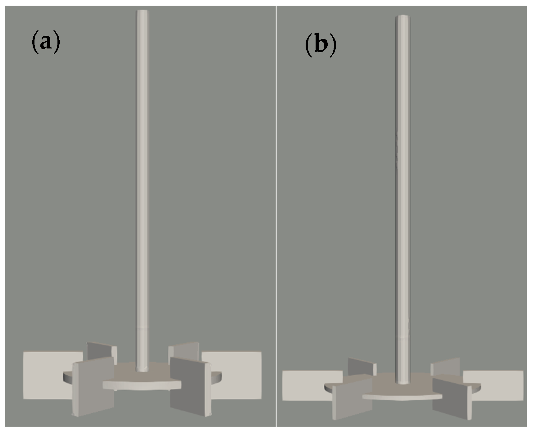
2.1. Model of a Simple Agitation Vessel

The system selected was a cylindrical unbaffled tank fitted with a RT. The geometry is obtained from [38], and some geometrical details are listed in

Table 1. Geometrical details of the CFD model of the simple agitation device.

Parameter	Value [m]
Diameter (D)	0.2286
Tank diameter (H)	0.46
Blade length (D/4)	0.05715
Blade length (D/8)	0.028575
Blade height (D/5)	0.04572
Blade thickness	0.00328
Shaft diameter (0.06D)	0.013716
Disk length (D/3)	0.0762
Disk thickness	0.00328
MRF length (4/3D)	0.3048
Clearance	0.15
Liquid height from RT	0.2286

and shown in Figure 1 for two CFD models using two blade lengths (additional details can be found in Supplementary Materials). The system involved the use of water and air as fluids with their properties obtained at room temperature (T = 20 °C; ${\rho }_{{\mathrm{H}}_2\mathrm{O}}$ ~ 1000 kg/m³; ${\mu }_{{\mathrm{H}}_2\mathrm{O}}$ ~ 0.001 $\mathrm{Pa}·\mathrm{s}$; ${\rho }_{air}$ ~ 1 kg/m³; ${\mu }_{air}$ ~ 1.48$·{10}^{-5}$ $\mathrm{Pa}·\mathrm{s}$, $P$ = 101,325 Pa), and its surface tension coefficient ($\sigma$) was taken as the standard literature value of 0.07 $\mathrm{N}·\mathrm{m}$.

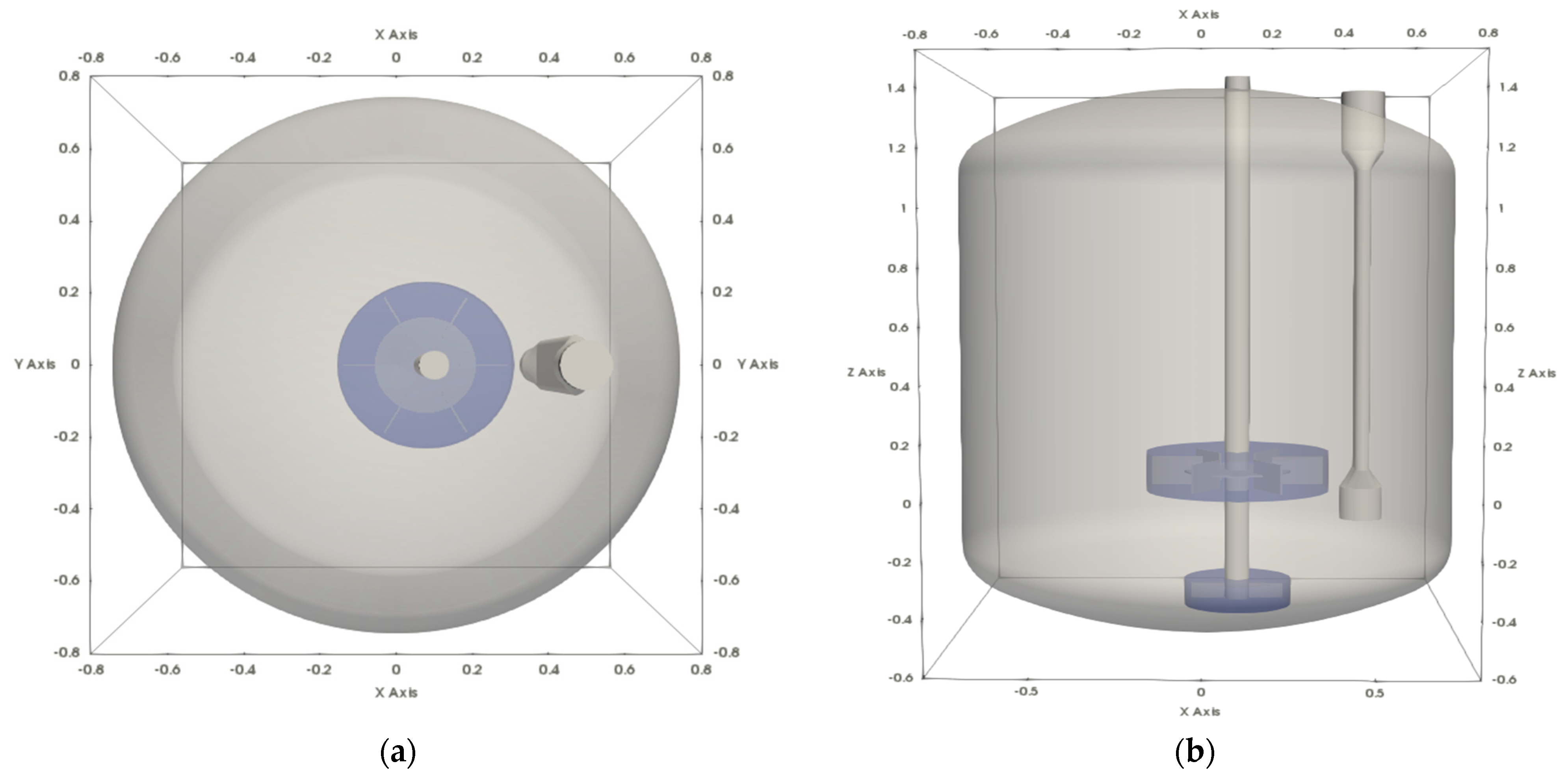
2.2. Model for the Industrial Reactor

The industrial reactor consists of a cylindrical vessel with two torispherical caps for the upper and bottom parts and is fitted with an eccentrically mounted agitation device consisting of a Rushton turbine and a bottom kicker impeller for solid resuspension. Additionally, it is equipped with a beaver-tail baffle parallel to the flow to avoid the disruption of the surface vortex. The hydrogenation reactor is operated in batch mode, involving the use of a solid-state suspended catalyst, and hydrogen is transferred continuously to the liquid phase by pressurising the reactor headspace. For a single batch, the hydrogenation reaction is performed in stages, in which the raw material is dosed and reacts in three portions. Therefore, the reaction volume increases with each portion added, and the impact of agitation rate on mass and heat transfer can vary significantly within a single batch. The system consists of methanol as solvent and hydrogen gas at the headspace. A volume of 1500 L was considered for the solvent (highest volume after the addition of the third portion of the raw material) with a constant temperature of 50 °C for both phases. The total hydrogen pressure was specified as 2.75 absolute bars. Methanol density and viscosity were specified as ${\rho }_{\mathrm{MeOH}}$ = $762$ kg/m³; ${\mu }_{\mathrm{MeOH}}$ = $3.9·{10}^{-4}$ $\mathrm{Pa}·\mathrm{s}$; hydrogen properties are specified as ${\rho }_{H_2}~0.209$ kg/m³; ${\mu }_{H_2}$ = $9.353·{10}^{-6}$ $\mathrm{Pa}·\mathrm{s}$ (Sutherland formula); and the rest of the thermophysical properties were assumed to be those of a perfect gas. The surface tension coefficient was taken from the Dortmund Data Bank [40] for air–methanol as ~0.02 $\mathrm{N}·\mathrm{m}$, and the bubble diameter was set to 5$·$10⁻⁴ m for the Schiller–Naumann drag force correlation.

In the first stage, the geometry of the industrial reactor was sketched from the design drawings and exported for mesh generation as shown in Figure 2. The main reactor dimensions for CFD modelling are summarised in

Table 2. Dimensions for the CFD model of the industrial reactor, where the centre of the reference axes is located at the bottom centre of the RT.

R101	(Dimensions in mm)
Diameter reactor (D)	1600
Height nozzle-to-nozzle	2039
Type of impeller	Rushton
$\mathrm{Diameter} \mathrm{impeller} ({\mathrm{D}}_{\mathrm{RT}}$)	560
Dimensions flat blade (Hb/Wb/thickness)	110/165/7.7 (0.06D)
RT flat plate (length/thickness)	173.55/22.4 (0.04D)
Distance from axis to internal part of blade	115
Number of flat blades	6
Distance from bottom	575
Shaft eccentricity	100 from centre reactor
Diameter shaft axis	80
Distance to top	1464
Distance to top hemispherical cap	1142
Distance to bottom hemispherical cap	269
MRF dimensions (diameter-height)	600–150
Type of impeller	Bottom kicker
Diameter impeller (Dkick)	300
Dimensions flat blade (height/thickness)	60 (Dkick/5)/4.6 (5Dkick/160)
Number of flat blades	2
Distance from bottom	70
Distance from RT	505
Shaft eccentricity	100 from centre reactor
MRF dimensions (diameter-height)	350–100
Type of baffle	Cylinder (C)-beavertail (B)-cylinder (C)
Distance from wall	295
Distance from RT centre	405
Lower part (length/width)	200/140 (C)
Middle part (length/width)	1150/180 (B)
Upper part (length/width)	300/140 (C)
Bottom connecting height (C to B)	75
Upper connecting height (B to C)	75

with an estimated total volume of 3.686 m³ and 3.659 m³ without internal elements.

In Figure 3, a cross-section of the mesh is shown with additional refinements close to the impellers and to the fluids’ interface (R3 in Table S2 in Supplementary Materials), where the top part of the reactor is excluded from the simulation by taking advantage of the total pressure boundary condition.

3. Mathematical Models

3.1. Modelling Approximations

A Eulerian 3D formulation of the phases was selected to properly resolve the interaction between phases and to predict the presence and size of the surface vortex as well as the bulk mixing. Thus, a higher cell density at the fluid interface was required to avoid large discontinuities and to compute accurately interfacial areas. Unsteady-state simulations were run at selected rotational speeds and time-averaged to obtain steady-state fields until monitored fields did not change with additional time stepping. Therefore, dynamic processes that occurred in the reactor (e.g., initial feed-sparging of hydrogen through the dip tube) were not considered. For the hydrogenation reactor, the solvent (methanol) and hydrogen were assumed to have constant properties during the simulation, where Newtonian properties were specified for both fluids and no thermal effects were considered. Two-equation Reynolds-averaged Navier–Stokes (RANS) turbulence models were selected. For comparison, the OpenFOAM (OF) implementation of the standard k-ε and the k-ω shear stress transport (SST) were used and assessed. Although more advanced turbulence models are available (e.g., LES or DES), these 2-eq. turbulence models are significantly computationally cheaper while being moderately accurate, which is sufficient for most industrial applications. Additionally, the multiple reference frame (MRF) approach was used to model the rotation of the impeller [16]. Using these assumptions, numerical simulations of the gas–liquid two-phase flow process were performed with OF v7 using the multiphaseEulerFoam solver, which combines the volume of fluid (VOF) approach with the classical Eulerian approach (see Supplementary Materials for a detailed description of the governing equations and model details).

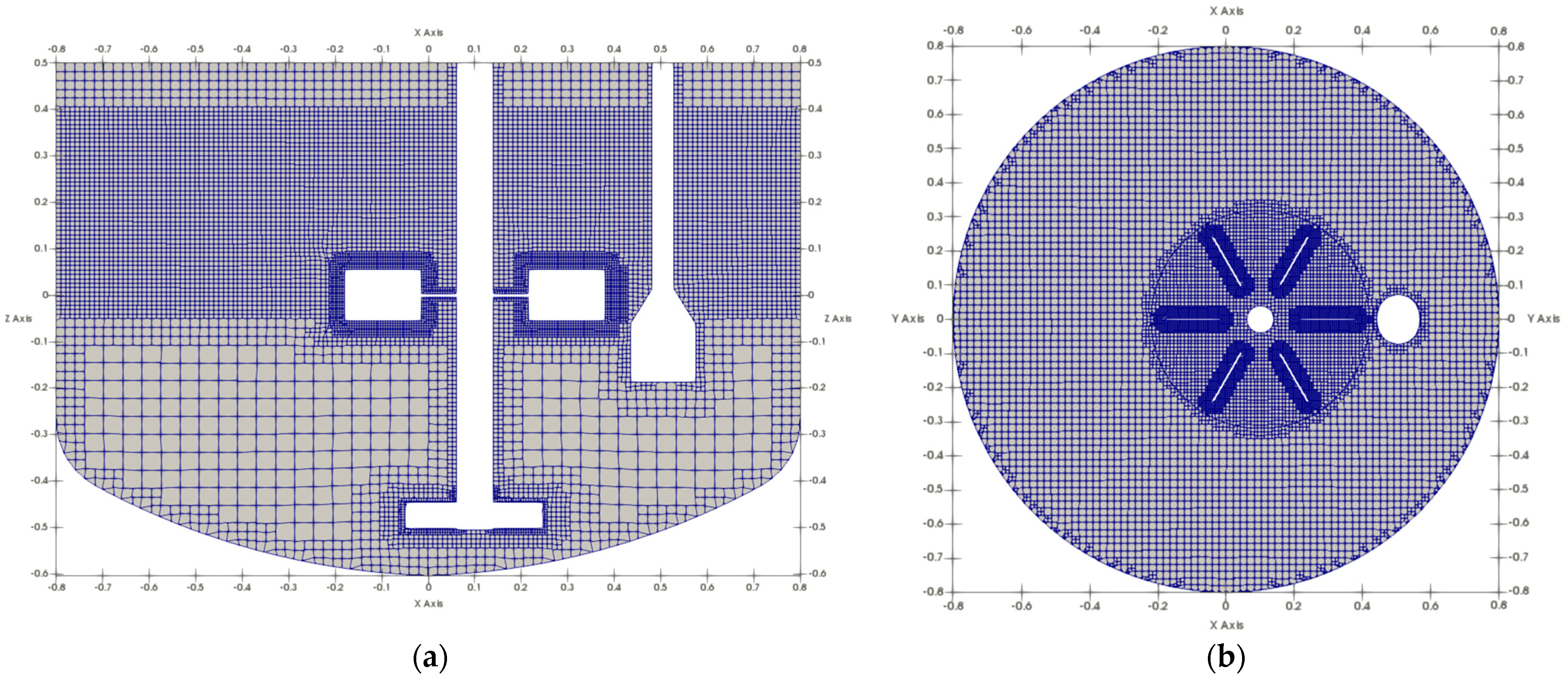
3.2. Solver Settings, Boundary Conditions, and Computational Resources

Some important solver settings for multiphaseEulerFoam are specified in

Table 3. Solver settings and models used.

Solver Name	multiphaseEulerFoam + MRF
Turbulence Models	$\mathrm{Standard} k-\epsilon$$\mathrm{and} k-\omega$ SST
Linear solvers	$\alpha$: Smoothsolver + Gauss-Seidel + MULES correction at interface Pressure: GAMG + Gauss-Seidel $\mathrm{U}/k/\epsilon /\omega$: Smoothsolver + GaussSeidel	Tolerances = 10−8 interfaceCompression = 1 Min.Iters = 3–5
Solver settings	PIMPLE solver	1 outer + 3 inner corrections + 1 non-orthogonal corrector
Discretisation schemes
Gradients	Default: Gauss linear	grad(U): cellMDLimited Gauss Linear 1
$\alpha$	Gauss vanLeer
Momentum	linearUpwindV grad(U)	Laplacian: Gauss linear limited 0.5
$k/\epsilon /\omega$	Gauss upwind	Laplacian: Gauss linear limited 0.5

. The numerical discretisation of momentum was second-order but bounded by limiters to avoid oscillations that would lead to divergence during the computation of the solution. Turbulent quantities were solved using first-order schemes since they are known to have a small effect on the mean velocity field. Correctors and limiters in Laplacian terms ensure the stability of the solver with unbounded solutions in high local cell nonorthogonality [41]. The initial $∆t$ was set to $5·{10}^{-6}$ s, but it was dynamically adjusted by the solver to ensure $\mathrm{Co}<1$ with a maximum allowed $∆t=0.01$ s.

Boundary conditions (BC) comprise all models that interact with the flow at the boundary limits of the system. For this system, the walls of the stirring tank were defined as the standard no-slip BC for all variables. For all turbulent variables, standard wall functions for both turbulence models were used. At the top patch of the stirring tank, a total pressure BC was specified ($P_{total}=250,000 \mathrm{Pa}$) to ensure a stable solution. The rest of the dynamic pressure boundary conditions were specified as fixedFluxPressure in all patches to ensure continuity at this location, as it automatically handles additional body forces such as gravity and surface tension at the walls. For α (volumetric cell phase fraction), a zero gradient was applied at the walls (equivalent to set alphaContactAngle 90° BC to ignore surface tension effects), and a uniform unity fraction value was specified at the top for pure hydrogen. Lastly, velocity BCs were specified as follows. A fluxCorrectedVelocity was applied to the top to recalculate velocity components to satisfy continuity based on the total specified dynamic pressure. The rest of the velocity BCs were zero-valued (including the MRF parts of the shaft and impeller). Outside of the MRF, the shaft has a constant rotatingWallVelocity clockwise rotational value equal to that of the rotational speed selected.

The calculations to carry out this work made use of the UGent Tier-2 cluster (1 node: 2 × 18-core Intel Xeon Gold 6140, Skylake @ 2.3 GHz). Approximately, the simulations required 1–3 nodes (aiming at ~20,000 cells/core) for 3–6 days depending on the simulation case and convergence requirements to establish the flow field and to collect meaningful statistics.

4. Results

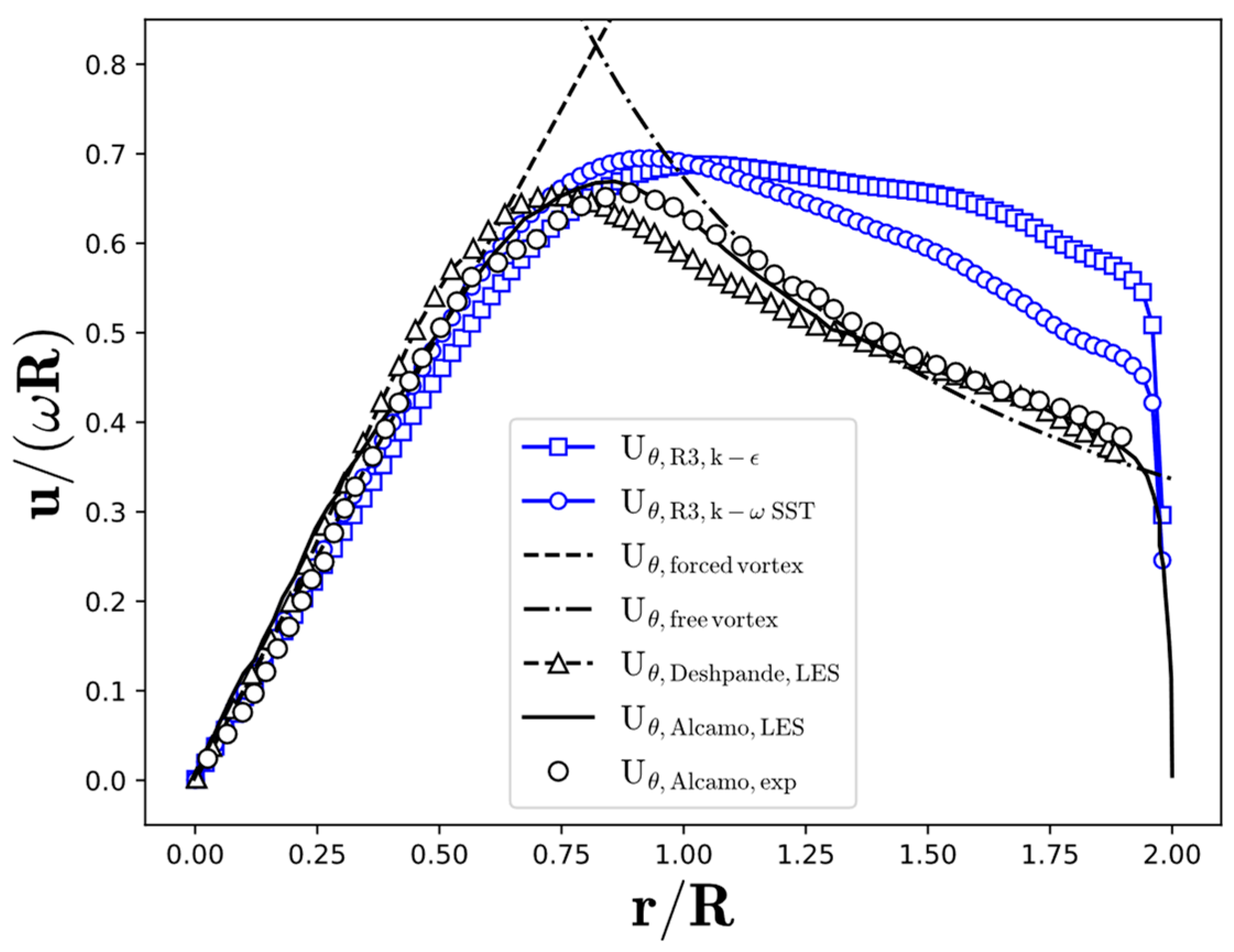
4.1. Simple Agitation Device

To assess the predictive capabilities of the industrial model, a comparison of the simple model performance is obtained for the air–water system. This is obtained using three quantities of interest (QOI): (1) impeller power consumption, (2) surface vortex depth, and (3) tangential velocity component radial profile. The results of the CFD model will be mainly compared with LES simulations from Deshpande’s et al. setup [38].

In stirred tanks, a useful quantity is the power number ($N_P$), which can be calculated as:

$$N_P=\frac{\mathrm{P}}{\rho N^3{D}_i{}^5}$$

(1)

where $\rho$ is the fluid density, $N$ is the impeller’s rotational speed, $D_i$ is the impeller diameter, and $\mathrm{P}=2\pi N\mathrm{T}$ is the power consumed by the impeller. In CFD, the torque ($\mathrm{T}$) can be obtained by the integration of all surface forces ($S$) in the rotational axis direction (pressure and viscous contributions).

$$\mathrm{T}={{\displaystyle \int }}_S^{}r\times \left[\rho \left(P-P_{ref}\right)·n+\rho \left(\upsilon +{\upsilon }_{turbulent}\right)\left(\nabla u+\nabla u^T\right)·n\right]dS$$

(2)

where $r$ and $n$ are the distance and surface normal cell vector, $P_{ref}$ is a reference pressure (defined kinematically), $\upsilon$ is the kinematic viscosity, and $\nabla u$ is the velocity gradient tensor. This integration is performed over all wall cells composing the impeller blades and shaft that contribute to the axial net torque. For each simulation, numerical convergence is assessed by running the simulation sufficiently long so that the mobile average reaches a sufficient steady-state value for the torque force and several velocities and pressure probes. Next, a mesh refinement study is performed, and two turbulence models are tested.

In Figure 4, it is observed that torque in R3 can be considered sufficiently refined. However, it is noted that the runs with the k-ε model tend to significantly overpredict the power required by the impeller compared to Deshpande’s value. In contrast, the $k-\omega$ SST model gives a more accurate prediction, but it is still not accurate enough (~20% difference). It is noted that in the work of [38] that the blades have a higher length with respect to the width. This affects the power drawn by the impeller since the cross-section of the blade is different, and it is known that the size and geometry of the impeller greatly affect the integration of forces [3]. A new run with the new blades (D/8) confirms that this is the case, achieving a more accurate value for the power number (~4%). The results of different CFD simulations are summarised in

Table 4. QOI for power number and vortex depth. Settings are $D$ =$Z_s$ (liquid height) = 0.2286 m, $N$ = 1.667 s⁻¹, $R{e}_D$ = 87,000, $F{r}_D$ = 0.065.

Refinement + Model	$N_p$	Rel. Diff. $N_p$[%](Deshpande)	Vortex Depth (${\delta }^{ *}/D$)	Rel. Diff. $\delta /D$[%]
[38]	0.55	-	0.35	-
[36] & $N_p=19.5R{e}^{-0.3}$ [12]	0.65	-	-	-
R1 + $k-\epsilon$ model	1.10	100%	0.34	2.18%
R2 + $k-\epsilon$ model	0.89	61.81%	0.37	6.19%
R3 + $k-\epsilon$ model	0.88	60%	0.38	9.56%
R3 +$k-\omega$ SST model	0.65	18.18%	0.388	11.06%
R3 D/8 blades + $k-\omega$ SST model	0.53	3.63%	0.399	14%

* δ: defined as the normalised distance between the highest and lowest point of the interface.

for the different QOIs.

The vortex depth constitutes an important QOI for model assessment, as it is directly related to the development of the surface vortex from the shaft. The vortex depth in Table 4 is obtained by performing an azimuthal average of the mean volumetric phase fraction (${\overline{\alpha }}_{r,solvent}=1/N_{cells}·{\displaystyle \sum }_{\theta =0}^{360}{\overline{\alpha }}_{r,\theta })$ in a radial (r)-axial (z) cross-section of the stirring tank. It is observed that the simulations successfully predict the development of the vortex and the shape of the vortex is in accordance with that reported by [38] (a partial hyperboloid shape). Since the phase fraction variable is a continuum field in CFD, the interface is obtained from the simulations as the phase’s boundary where there is the greatest transition ($\alpha$ ~ 0.5). An evaluation of the different runs presents an estimated relative difference of ~10% for the finer meshes, which is considered sufficient.

The surface vortex is the result of the equilibrium of fluid forces at both sides because of a solid body movement around the rotational axis. Results of the surface vortex are presented in Figure 5 by plotting the dynamic pressure field ($P_{rgh}=P-\rho gh$). As can be observed, a lower $P_{rgh}$ value around the shaft seems to drive the development of the surface vortex.

The theoretical description of a vortex depth in an unbaffled tank has been formulated by [13]. When viscous effects are not important and assuming a purely tangential flow, the radial profile of the tangential velocity component reads as:

$$\{\begin{array}{c}{u}_{\theta }=r·\omega ,\mathrm{for}<R_c:\mathrm{forced} \mathrm{vortex}\\ u_{\theta }=\frac{R_c{}^2·\omega }{r},\mathrm{for}<\frac{T}{2}:\mathrm{free} \mathrm{vortex}\end{array}$$

(3)

It consists of two regions. The first part is called “forced vortex”, where the fluid moves with constant angular velocity (so there is no mean shear). This section moves as a “solid body rotation” until a certain critical radius denoted as $R_c$. Beyond this radius, there is a second region called “free vortex”, where the fluid moves at constant angular momentum. As a result, the tangential component decays until it reaches the wall. It is worth noting that in these types of systems, the following applies: $u_{\theta }\gg u_r,u_z.$

To assess the validity of the simulations, data of the phase-averaged tangential velocity component along the radial profile are compared in Figure 6 with data from [36,38]. As expected, the data from the literature follow the theoretical model of Equation (11) very well, with an approximate $R_c/R$ = 0.75. The CFD simulations using RANS models predict very well the “forced vortex” region with a linear increase. However, both turbulence models overestimate the “free vortex” in a consistent manner and delay the switch from one region to the other (as seen by the highest tangential component location). The difference in performance between LES and RANS simulations is commonly attributed to an incorrect prediction of turbulent viscosity in the region of high swirl motion since these models are oblivious to streamline curvature and swirling motion effects (influencing the development of turbulence). This limitation has been confirmed and reported multiple times in literature, even for unbaffled stirred tanks (see [32]).

With these results, the CFD model used in this study is demonstrated to be capable of simulating the main flow physics for surface vortexing in unbaffled stirred tanks with RTs. Therefore, the multiphaseEulerFoam solver coupled with the MRF approach and the SST turbulence model will be used for the development of the industrial stirring tank model. The selection of the $k-\omega$ SST model is based on predicting more accurately the power consumption and the good agreements in terms of tangential velocity and surface vortex depth.

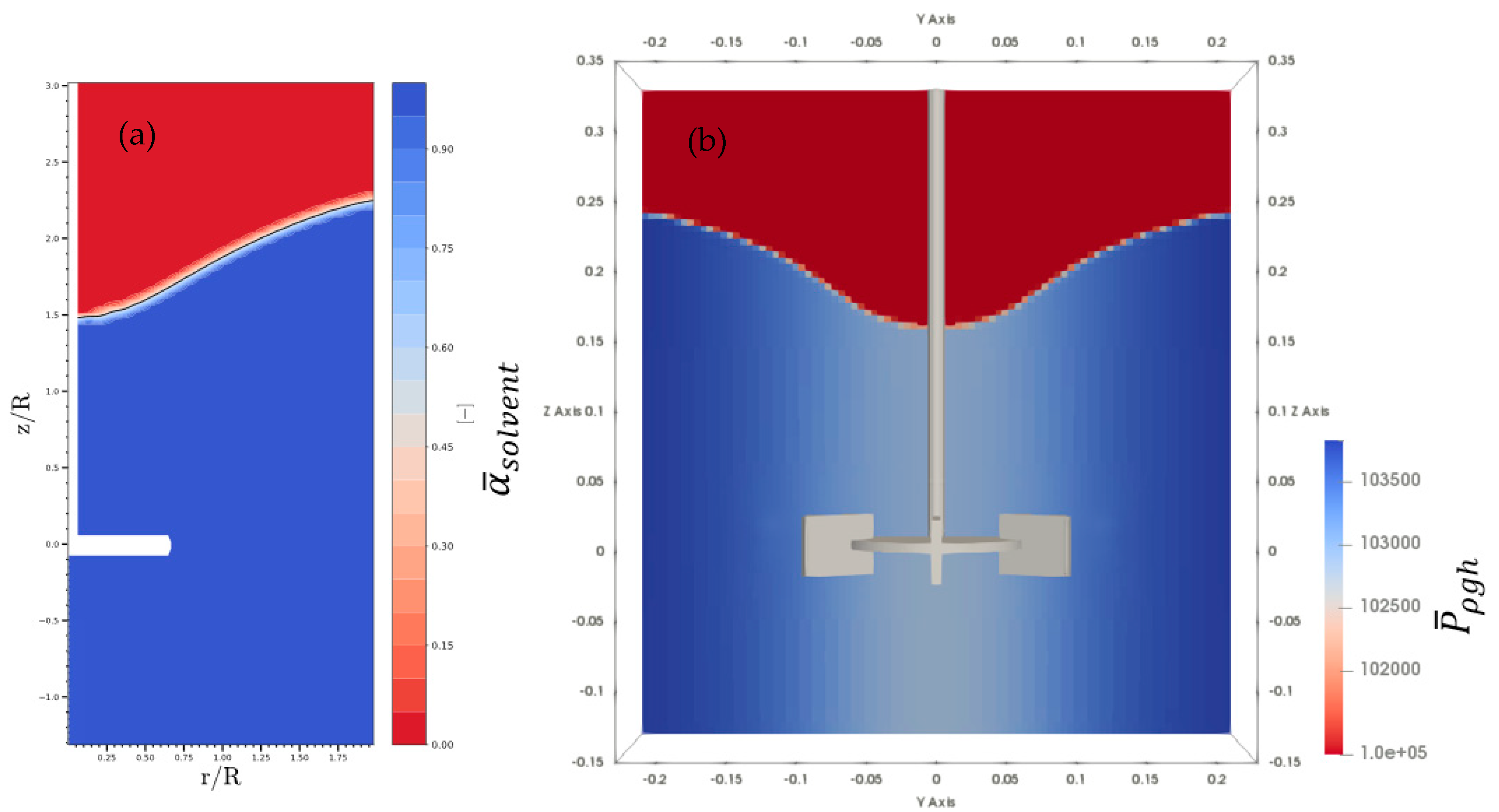
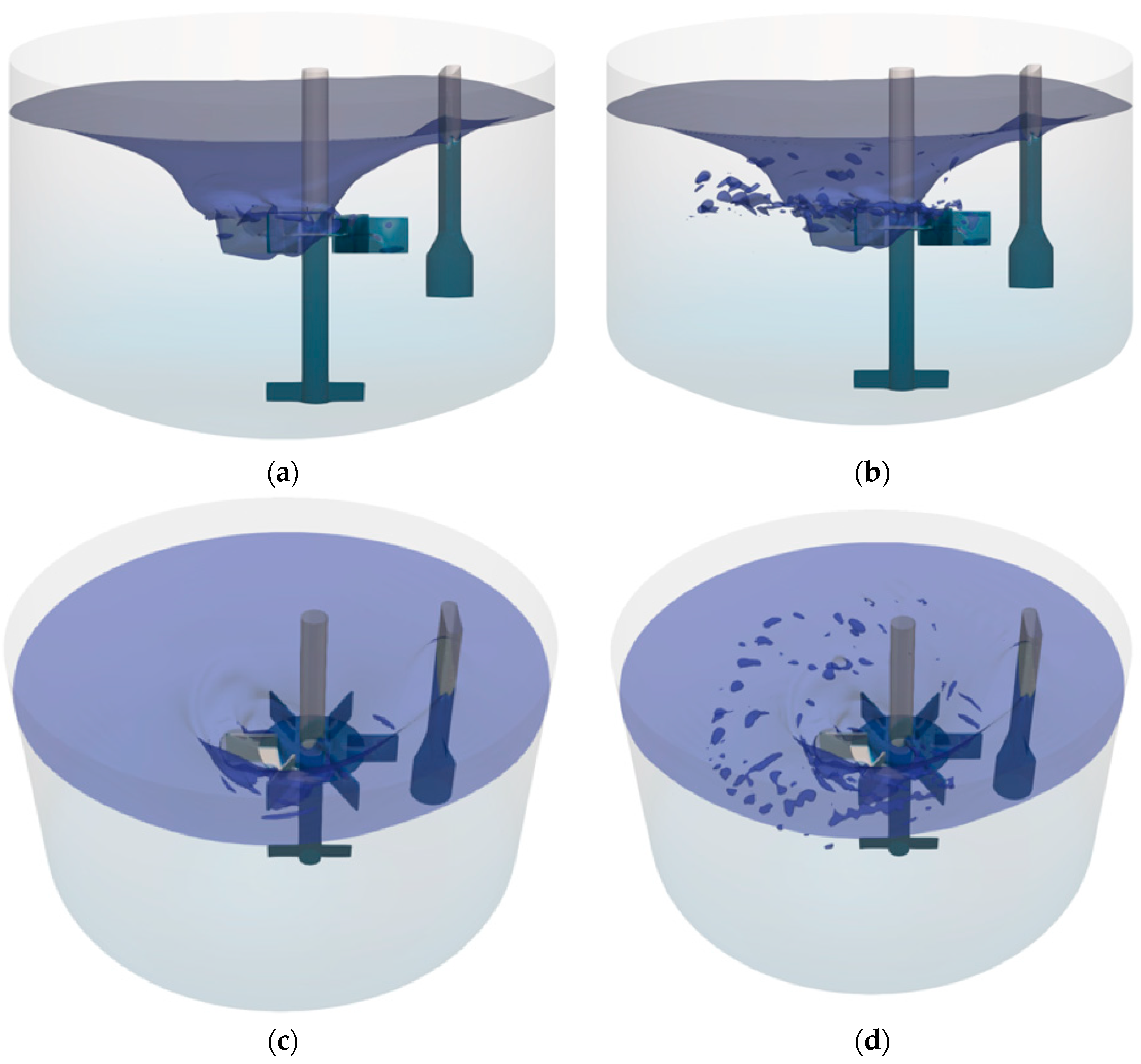
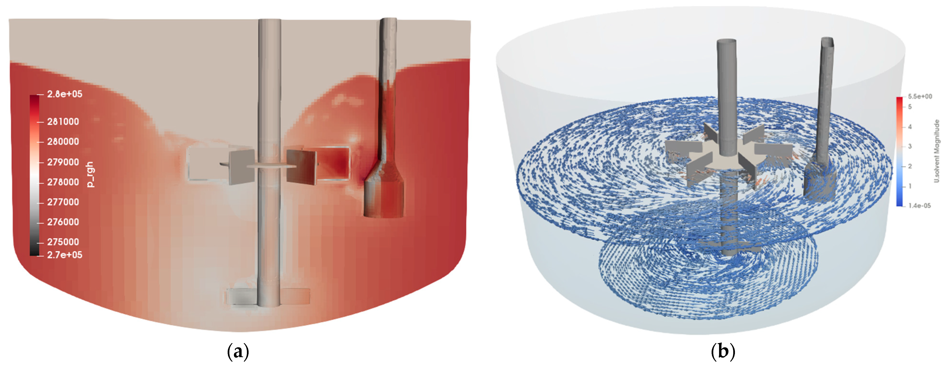
4.2. Industrial Reactor

A series of CFD simulations are performed to investigate mixing and mass transfer capabilities for the hydrogenation industrial reactor described in Section 2.2. Firstly, the main flow features of a reference CFD simulation are analysed. Secondly, a series of CFD runs is presented to obtain potential mass transfer surface areas as a function of different rotational speeds and solvent volumes. Finally, a series of tracer tests are presented for a mixing study.

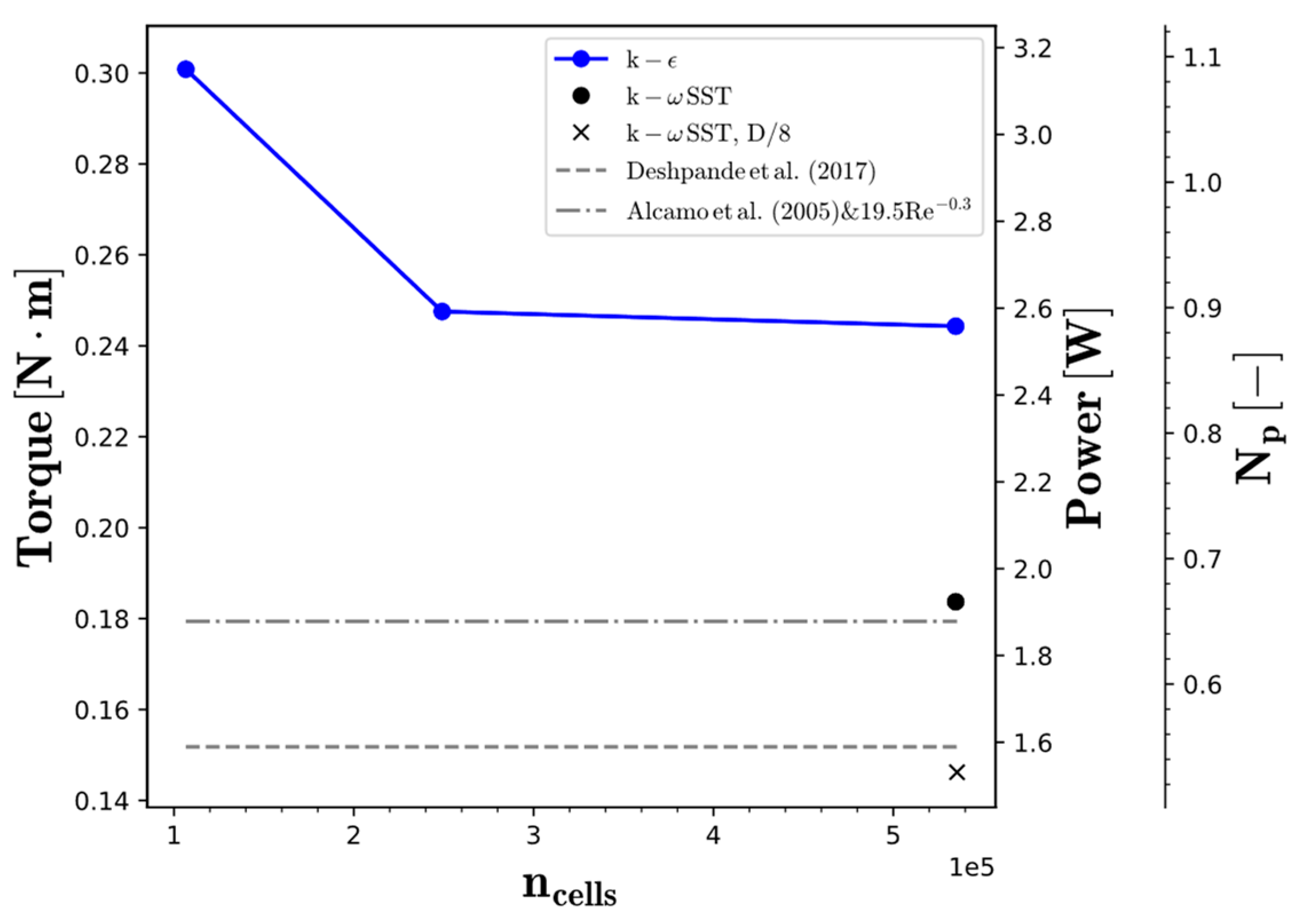
4.2.1. Mesh Independency Test

A mesh independence test is carried out to evaluate the appropriateness of the meshes used with respect to the errors in the spatial discretization involved in the simulation of the industrial tank. The mesh details are summarised in Table S2 (in Supplementary Materials), and the results of mesh refinement on two relevant QOI’s (time-averaged surface area and agitation power consumption) with four meshes are shown in Figure 7.

As can be seen in Figure 8, a mesh of $1.2·{10}^6$ cells (R3) can be considered suitable to be used for the simulations at the industrial scale of two relevant QOIs since it shows near-asymptotic behaviour. Since these simulations are transient, the use of R3 is selected for its balance between accuracy and computational resources needed. Although not shown, other cases operating at higher rpm are modified to increase their mesh density to ensure a sufficient mesh refinement at the surface and near the RT impeller.

4.2.2. Reference Case

A clockwise rotational speed of 100 rpm is fixed with the initial solvent surface being stationary and flat. Convergence is obtained for each simulation after monitoring torque, and several velocity and pressure probes to reach steady-state fields that no longer change with additional time steps.

Figure 8 visualises the surface of the solvent by plotting the contour levels of ${\alpha }_{solvent}=0.5$. After 90 s rotating at 100 rpm, the CFD simulation predicts that the surface vortex reaches the impeller and entrains the gas phase into the solvent. Gas bubbles are entrained and are radially dispersed by the RT. However, the gas bubbles seem to be confined within the impeller region due to the solid body rotation movement of the fluid. The presence of the internal baffle does not disrupt the development of the vortex, and its use is primarily associated with promoting bulk mixing.

In Figure 9, the pressure contours indicate the development of a lower pressure region near the axis of rotation, which induces the development of the surface vortex (resembling that of Figure 5). In Figure 9 (right), the velocity vectors at two different axial locations confirm the circular type of rotation in most of the tank. The main reason is that the two impellers consist of flat blades perpendicular to the flow, which both contribute to sustaining the circular motion observed as well as to providing local mixing in their vicinity.

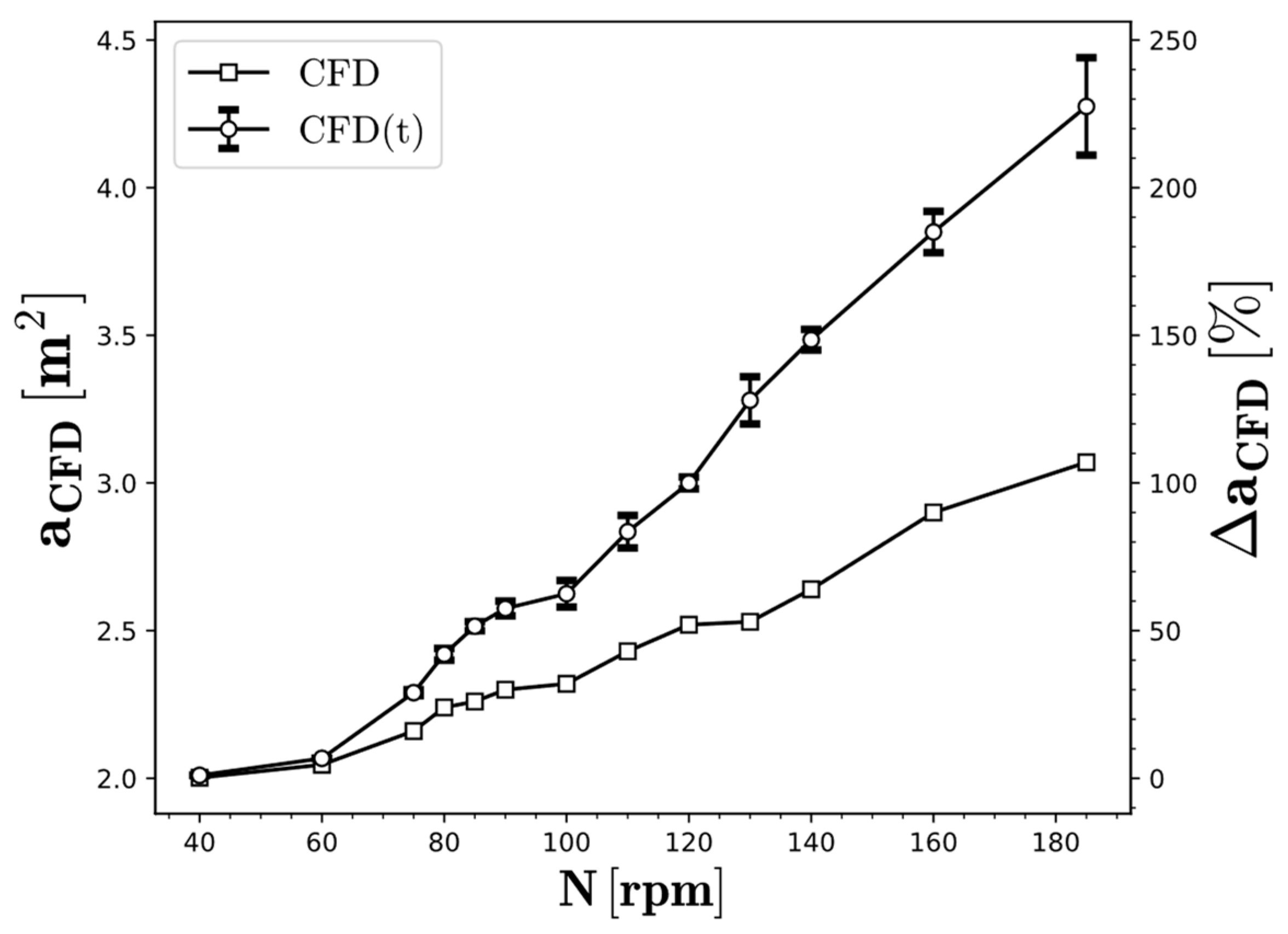
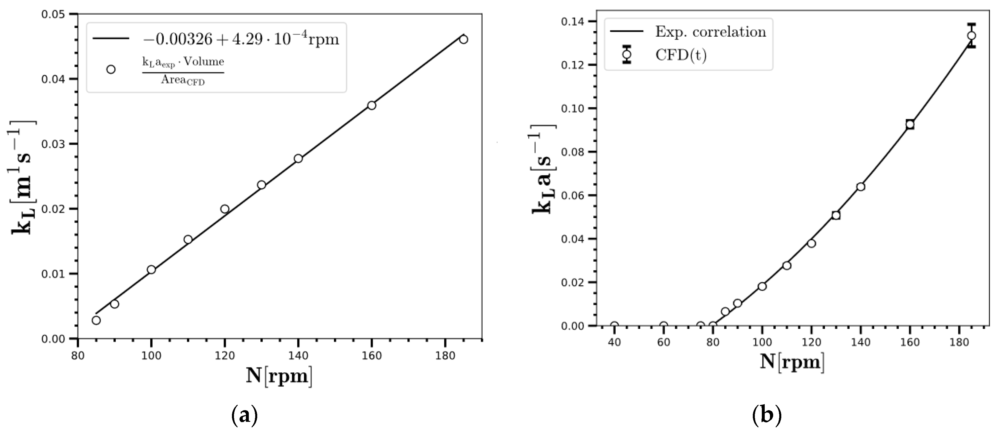
4.2.3. Mass Transfer Area vs. Rotational Speed

In hydrogenation, mass transfer of hydrogen from the headspace to the solvent bulk is one of the main limiting processes, as mentioned in Section 1. Directly modelling the mass transfer process would require a mass transfer model in CFD and tracking the hydrogen concentration in both phases to calculate hydrogen mass transfer fluxes. Although different modelling approaches are available, it was instead decided to focus on simply computing the surface contact area between phases (at ${\alpha }_{solvent}=0.5$). This area is expected to be potentially linked with mass transfer coefficients and offer a simpler and computationally cheaper option for the study of industrial reactors. Thus, different CFD runs were performed to obtain an estimation of the readily available mass transfer area at different rotational speeds. The results are shown in Figure 10.

Figure 10 shows that increasing the rotational speed of the agitation device leads to different increases in area with respect to a flat liquid surface. The onset for this difference is observed to appear between 60–75 rpm (with ~10%$·a_{CFD}$), where the RT starts to become flooded since the surface vortex reaches the impeller. The area computed from mean fields only considers the surface area from the vortex, whereas the areas computed from time-averaging instantaneous fields take into account entrained gas. As a result, a sudden increase in mass transfer area is obtained since the surface vortex reaches the RT, and gas is entrained and further dispersed into the bulk (achieving values as high as 220% $∆a_{CFD}$).

In order to relate areas with mass transfer coefficients, a correlation is necessary to compute the liquid mass transfer coefficient ($k_L$). For this volume, data for $k_{L}a$ values were experimentally available (Equation (12), for $80\le \mathrm{rpm}\le 185$) and are used to estimate $k_L$k_L values from Equation (13):

$$k_{L}a=A·{\mathrm{rpm}}^2+B·\mathrm{rpm}+C=4·{10}^{-6}{\mathrm{rpm}}^2+1.86·{10}^{-4}\mathrm{rpm}-0.04$$

(4)

$$k_L=k_L{a}_{exp.}·\frac{\mathrm{V}}{a_{CFD}}$$

(5)

From Figure 11, it can be observed that $k_L$ can be fitted linearly as a function of the impeller rotational speed. The calibration from Figure 11 does not readily imply that the real $k_L$ should be a linear function of the agitation rate. It is possible that inaccuracies in computing $a_{CFD}$ can be compensated by this linear fit (especially since high $k_L$ values are obtained [42]). However, it is still possible that $k_L$ should be a function of the agitation device. For instance, various $k_L$ correlations do not only depend on the diffusion coefficient, but they mostly include some dependencies with dissipated energy from the agitation device [43].

Nevertheless, from this calibration, it is estimated that very low values of $k_{L}a$ are achieved for rotational speeds below impeller flooding (<0.01 s⁻¹ for < 75–80 rpm). This is in partial accordance with the experimental correlation showing that at <75–80 rpm, the impeller is not yet flooded and cannot provide values of $k_{L}a>0.01$ s⁻¹ (since there is not yet gas entrainment, which is believed to be the main driving force for high mass transfer values in this reactor configuration). The range of relatively moderate $k_{L}a$ values achieved ([10⁻²–10⁻¹ s⁻¹] compared to other reactor configurations achieving [10⁻¹–1 s⁻¹]) suggests the use of this reactor configuration for highly exothermic or fast reactions [3]. Based on Figure 11, accurate control of the reaction exothermicity can then be performed by dynamically adjusting the rotational speed.

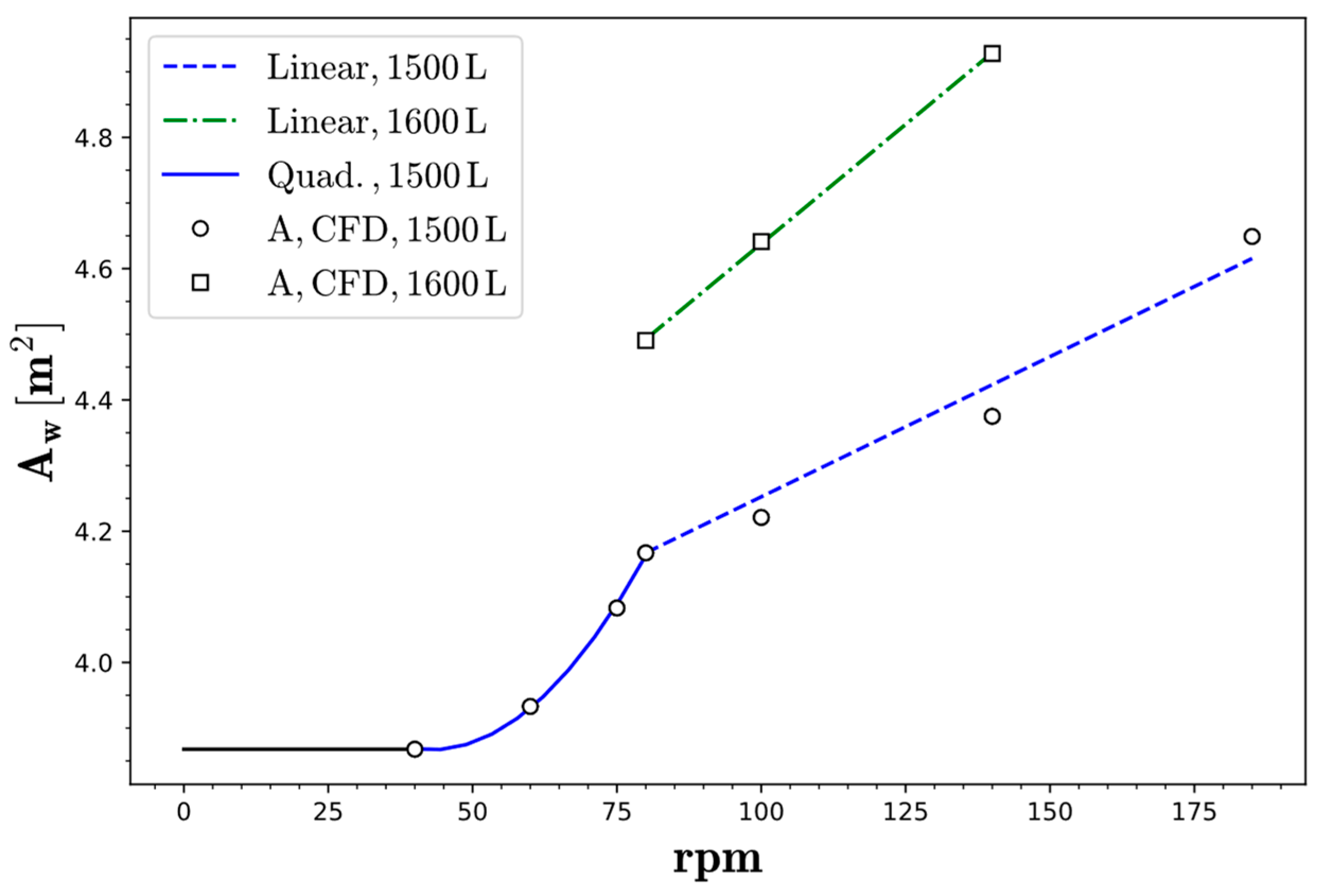
4.2.4. Wetting Area vs. Rotational Speed

In hydrogenation, the available area for direct exchange of heat transfer is an important variable when considering the design, control, and kinetic modelling of the system. For instance, the amount of heat that can be extracted from the system is directly proportional to the available heat exchange area ($Q_{heat}=UA\left(T_{wall}-T_{HE}\right)$). For this system, heat is removed with a jacketed vessel with half-pipe coil jackets around the reactor. Therefore, the total available area for heat transfer is obtained from the total wetting area of the liquid contained in the reactor (${\mathrm{A}}_{\mathrm{w}}$ = area of bottom toroid (0.987 m²) + area of cylinder). Since the wetting area is a function of the rotational speed, CFD is used to predict this dependence and to establish the appropriate correlations.

In Figure 12, for V = 1500 L, two different regions are observed. At low rpm, there is a high increase in area as a consequence of the development start of the surface vortex (which can be modelled quadratically). Once the surface vortex is established, a linear relation is observed within the rpms considered. The linear relation is also predicted for a higher liquid volume in the tank (V = 1600 L), and it is also observed to have a higher slope compared to V = 1500 L.

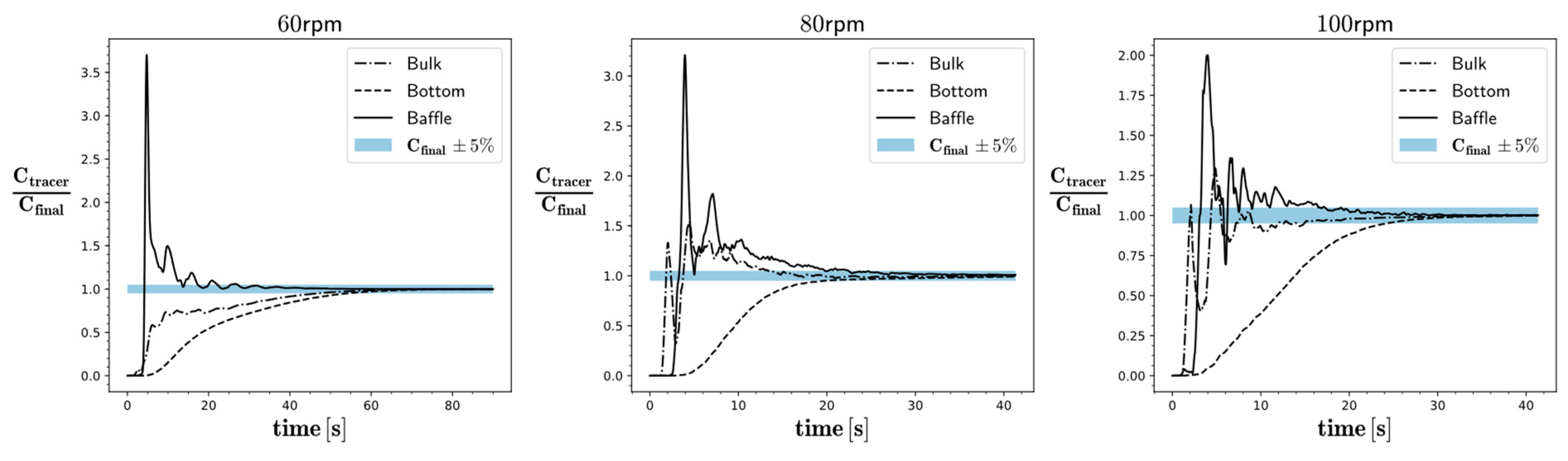
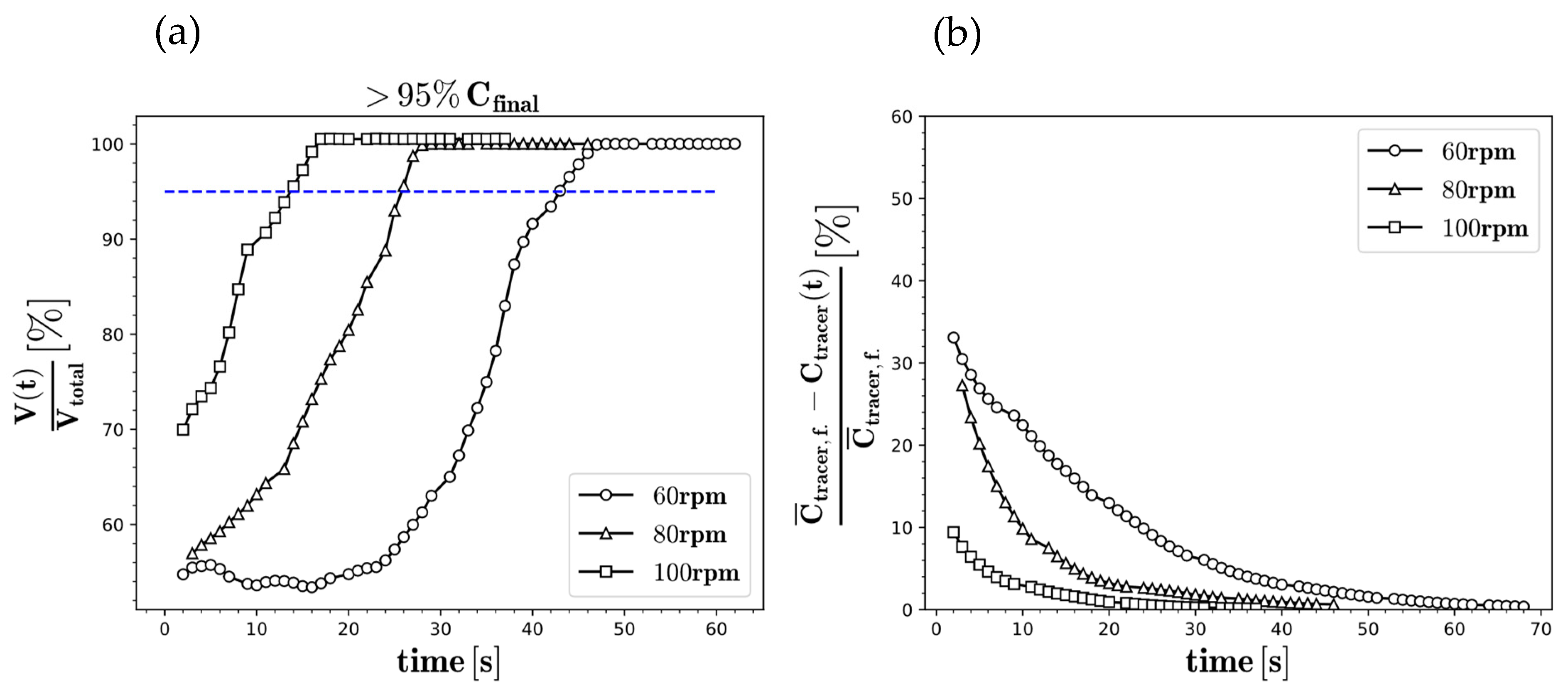
4.2.5. Blend Time Analysis

Mixing time is an important variable in hydrogenation as it is necessary to minimise the degree of nonuniformity of species and temperature to avoid gradients that could negatively impact process performance. Although several definitions are available, in this study, the mixing time (${\theta }_{95\%}$) will be defined as the time required for a tracer to reach 95% homogenisation.

In CFD, the mixing time (${\theta }_{95\%}$) can be estimated by solving over time the transport equation of an added passive tracer (Equation (6)).

$$\frac{\partial \rho {\alpha }_l\varphi }{\partial t}+\nabla \rho {\alpha }_{l}U\varphi =\nabla \rho {\alpha }_l\Gamma \nabla \varphi$$

(6)

where $\rho$ is the fluid density, ${\alpha }_l$ is the solvent phase-fraction, $\varphi$ is the scalar tracer, and $\Gamma =\left({\Gamma }_{mol.}+{\Gamma }_{t.}\right)$ is the general diffusion coefficient which can be modelled in CFD by decomposing it into a molecular and a turbulent eddy component:

$$\Gamma =\frac{1}{S{c}_{mol.}}+\frac{1}{S{c}_{t.}}=\frac{\mu }{\rho D_{mol.}}+\frac{1}{S{c}_{t.}}$$

(7)

where $S{c}_{mol.}$ and $S{c}_{t.}$ are the molecular and turbulent Schmidt numbers respectively, and $D_{mol.}$ is the diffusion of the tracer in the fluid. In absence of information, it is assumed that standard literature values of $D_{mol.}={10}^{-9} \left[{\mathrm{m} \mathrm{s}}^{-2}\right]$ and $S{c}_{t.}=0.7$ apply to specify the behaviour of the virtual tracer [44].

First, the time-evolution of tracer concentration is plotted in Figure 13 at three different spatial locations considering V = 1500 L. The first probe is representative of the bulk concentration of the reactor (x, y, z = −0.5, 0, −0.25); the second is located at the bottom, close to the kicker (0, 0, −0.55); and the third is located between the baffle and the tank wall (0.65, 0, 0). A small initial pocket of tracer is placed close to the impeller tip, and then the simulation advances in time, solving Equation (6) until the tracer fully dilutes into the fluid solvent. The location of the tracer is selected near the RT impeller since it is expected to behave similarly to a pocket of hydrogen that has been recently entrained at the vortex tip.

In Figure 13, the higher the rotational speed, the lower the time needed for these concentration profiles to achieve their final concentration value as expected. Between these rotational speeds, the concentration profiles at the same locations also show similar behaviour, indicating that the bottom part of the reactor takes longer to homogenise the tracer injection. This is directly shown in Figure 13, as the bottom part always requires a longer time to reach 95% of the value of the final concentration. Since the mixing time obtained from Figure 13 would depend on the location of the probe, we decided that we would also perform a volume integration of the tracer concentration. The integration monitors all cells that contain at least ≥95% of the final tracer concentration as a function of time, as is shown in Figure 14.

From Figure 14, ${\theta }_{95\%}$ can be determined as 47, 26, and 16 s for 60, 80, and 100 rpm, respectively, as indicated by the data surpassing the 95% volume occupancy. For these cases, the relative differences at ${\theta }_{95\%}$ were 1.76, 1.61, and 1.31%, respectively, suggesting that the contents can be considered sufficiently homogeneous for mixing applications.

Based on the results of Figure 13 and Figure 14, it is observed that proper mixing in this configuration can be achieved when there is sufficiently vertical homogenisation. This is expected, as the surface vortex and the use of the RT promote circular and radial dispersion, but not as much for axial dispersion. This suggests the use of other types of impellers that could promote axial mixing (if sufficiently high-mass transfer values can be ensured at reasonable power consumptions). However, it is also noted that H₂ entrainment would no longer occur from the surface vortex, but from a wavy solvent surface, which would be more challenging to model.

5. Conclusions and Perspectives

In this work, a CFD model has been developed to simulate an industrial hydrogenation reactor. The results show that the model is able to predict, as a function of rotational speed, the development of a surface vortex around the impeller’s shaft. The model was used to test new scenarios, with lower effort and resources, that would otherwise not be possible due to process constraints or safety regulations. By performing these types of simulations, important quantities for hydrogenation were virtually evaluated to aid in the operation and process control as well as to explore new designs and test optimization strategies. More specifically, the reactor’s capabilities to transfer hydrogen from the headspace to the solvent are shown to be a function of the size of the surface vortex, as it provides the available interfacial area for mass transfer. The results of these simulations were then used to develop novel process correlations to estimate variables, such as interfacial area for mass transfer and liquid height for heat exchange calculations, and to estimate mixing bulk times.

Despite already being a mature modelling framework that can bring a great deal of value, in order for CFD to become even more widely adopted and accepted in the pharmaceutical industry, further efforts could be made to assess the accuracy of the different CFD submodels and provide even higher trust. This can be achieved by performing dedicated measuring campaigns to facilitate sampling by smart reactor design and online Process Analytical Tools (PAT) to monitor evolving concentrations and properties. As previously discussed, the CFD model can also be improved by introducing more modelling complexity or modelling scenarios of interest. Additional complexity can be achieved by explicitly modelling H₂ mass transfer coupled with kinetics and heat release, simulating agitation by the sliding mesh (SM) approach, including population balance models (PBM), or by performing LES simulations to obtain more accurate fields. Other useful scenarios could be tested such as to study the influence of substrate/catalyst dosing or using CFD models to build reduced order models (ROM).

To conclude, CFD should not be viewed as a replacement of existing and well-established methodologies, but rather as a complementary tool that will prove in the future to be more useful in the pharmaceutical industry by bringing additional knowledge and allowing researchers to make the current methodologies more accurate.

References

1. Machado, R.M. Fundamentals of Mass Transfer and Kinetics for the Hydrogenation of Nitrobenzene to Aniline. ALR Appl. Note 2007, 1, 1–14. [Google Scholar]
2. Lee, S.-Y.; Tsui, Y.P. Succeed at Gas/Liquid Contacting. Chem. Eng. Prog. 1999, 95, 23–49. [Google Scholar]
3. Paul, E.L.; Atiemo-Obeng, V.A.; Kresta, S.M. Handbook of Industrial Mixing: Science and Practise; Wiley: Hoboken, NJ, USA, 2004. [Google Scholar]
4. Rylander, P.N. Hydrogenation and Dehydrogenation. In Ullmann’s Encyclopedia of Industrial Chemistry; Wiley: New York, NY, USA. [CrossRef]
5. Cho, H.B.; Park, Y.H. The effects of impeller characteristics in the hydrogenation of aniline on Ru/C catalyst. Korean J. Chem. Eng. 2003, 20, 262–267. [Google Scholar] [CrossRef]
6. Babnik, S.; Erklavec-Zajec, V.; Oblak, B.; Likozar, B.; Pohar, A. A Review of Computational Fluid Dynamics (CFD) Simulations of Mixing in the Pharmaceutical Industry. Biomed. J. Sci. Tech. Res. 2020, 27, 20732–20736. [Google Scholar]
7. Horner, M.; Joshi, S.; Waghmare, Y. Process Modeling in the Biopharmaceutical Industry; Elsevier Ltd.: Amsterdam, The Netherlands, 2017; Volume d. [Google Scholar]
8. Ramírez-Muñoz, J.; Martínez-de-Jesús, G.; Soria, A.; Alonso, A.; Torres, L.G. Assessment of the effective viscous dissipation for deagglomeration processes induced by a high shear impeller in a stirred tank. Adv. Powder Technol. 2016, 27, 1885–1897. [Google Scholar] [CrossRef]
9. Wu, H. An issue on applications of a disk turbine for gas-liquid mass transfer. Chem. Eng. Sci. 1995, 50, 2801–2811. [Google Scholar] [CrossRef]
10. Penicot, P.; Muhr, H.; Plasari, E.; Villermaux, J. Influence of the Internal Crystallizer Geometry and the Operational Conditions on the Solid Product Quality. Chem. Eng. Technol. 1998, 21, 507–514. [Google Scholar] [CrossRef]
11. Scargiali, F.; Busciglio, A.; Grisafi, F.; Brucato, A. Oxygen transfer performance of unbaffled stirred vessels in view of their use as biochemical reactors for animal cell growth. Chem. Eng. Trans. 2012, 27, 205–210. [Google Scholar]
12. Scargiali, F.; Busciglio, A.; Grisafi, F.; Tamburini, A.; Micale, G.; Brucato, A. Power consumption in uncovered unbaffled stirred tanks: Influence of the viscosity and flow regime. Ind. Eng. Chem. Res. 2013, 52, 14998–15005. [Google Scholar] [CrossRef]
13. Nagata, S. Mixing: Principles and Applications; Halstead-John Wiley: New York, NY, USA, 1975. [Google Scholar]
14. Rieger, F.; Ditl, P.; Novak, V. Vortex Depth in Mixed Unbaffled vessels. Chem. Eng. Sci. 1978, 34, 397–403. [Google Scholar] [CrossRef]
15. Markopoulos, J.; Kontogeorgaki, E. Vortex depth in unbaffled single and multiple impeller agitated vessels. Chem. Eng. Technol. 1995, 18, 68–74. [Google Scholar] [CrossRef]
16. Torré, J.P.; Fletcher, D.F.; Lasuye, T.; Xuereb, C. An experimental and computational study of the vortex shape in a partially baffled agitated vessel. Chem. Eng. Sci. 2007, 62, 1915–1926. [Google Scholar] [CrossRef]
17. Busciglio, A.; Caputo, G.; Scargiali, F. Free-surface shape in unbaffled stirred vessels: Experimental study via digital image analysis. Chem. Eng. Sci. 2013, 104, 868–880. [Google Scholar] [CrossRef]
18. Rao, A.R.; Kumar, B.; Patel, A.K. Vortex behaviour of an unbaffled surface aerator. Sci. Asia 2009, 35, 183–188. [Google Scholar]
19. Scargiali, F.; Tamburini, A.; Caputo, G.; Micale, G. On the assessment of power consumption and critical impeller speed in vortexing unbaffled stirred tanks. Chem. Eng. Res. Des. 2017, 123, 99–110. [Google Scholar] [CrossRef]
20. Galletti, C.; Pintus, S.; Brunazzi, E. Effect of shaft eccentricity and impeller blade thickness on the vortices features in an unbaffled vessel. Chem. Eng. Res. Des. 2009, 87, 391–400. [Google Scholar] [CrossRef]
21. Yoshida, M.; Wakura, Y.; Yamagiwa, K.; Ohkawa, A.; Tezura, S. Liquid flow circulating within an unbaffled vessel agitated with an unsteady forward-reverse rotating impeller. J. Chem. Technol. Biotechnol. 2010, 85, 1017–1022. [Google Scholar] [CrossRef]
22. Galletti, C.; Brunazzi, E. On the main flow features and instabilities in an unbaffled vessel agitated with an eccentrically located impeller. Chem. Eng. Sci. 2008, 63, 4494–4505. [Google Scholar] [CrossRef]
23. Assirelli, M.; Bujalski, W.; Eaglesham, A.; Nienow, A.W. Macro- and micromixing studies in an unbaffled vessel agitated by a Rushton turbine. Chem. Eng. Sci. 2008, 63, 35–46. [Google Scholar] [CrossRef]
24. Ciofalo, M.; Brucato, A.; Grisafi, F.; Torraca, N. Turbulent flow in closed and free-surface unbaffled tanks stirred by radial impellers. Chem. Eng. Sci. 1996, 51, 3557–3573. [Google Scholar] [CrossRef]
25. Serra, A.; Campolo, M.; Soldati, A. Time-dependent finite-volume simulation of the turbulent flow in a free-surface CSTR. Chem. Eng. Sci. 2001, 56, 2715–2720. [Google Scholar] [CrossRef]
26. Glover, G.M.C.; Fitzpatrick, J.J. Modelling vortex formation in an unbaffled stirred tank reactors. Chem. Eng. J. 2007, 127, 11–22. [Google Scholar] [CrossRef]
27. Jahoda, M.; Moštěk, M.; Fořt, I.; Hasal, P. CFD simulation of free liquid surface motion in a pilot plant stirred tank. Can. J. Chem. Eng. 2011, 89, 717–724. [Google Scholar] [CrossRef]
28. Yamamoto, T.; Fang, Y.; Komarov, S.V. Surface vortex formation and free surface deformation in an unbaffled vessel stirred by on-axis and eccentric impellers. Chem. Eng. J. 2019, 367, 25–36. [Google Scholar] [CrossRef]
29. Rajavathsavai, D.; Khapre, A.; Munshi, B. Numerical Study of Vortex Formation inside a Stirred Tank. Int. J. Chem. Mol. Nucl. Mater. Metall. Eng. 2014, 8, 1470–1475. [Google Scholar]
30. Yang, F.L.; Zhou, S.J. Effect of gravity on the hydrodynamics in an unbaffled stirred vessel. Chem. Eng. Technol. 2015, 38, 819–826. [Google Scholar] [CrossRef]
31. Li, L.; Xu, B. Numerical simulation of hydrodynamics in an uncovered unbaffled stirred tank. Chem. Pap. 2017, 71, 1863–1875. [Google Scholar] [CrossRef]
32. Haque, J.N.; Mahmud, T.; Roberts, K.J.; Rhodes, D. Modeling turbulent flows with free-surface in unbaffled agitated vessels. Ind. Eng. Chem. Res. 2006, 45, 2881–2891. [Google Scholar] [CrossRef]
33. Armenante, P.M.; Luo, C.; Chou, C.-C.; Fořt, I.; Medek, J. Velocity profiles in a closed, unbaflled vessel: Comparison between experimental LDV data and numerical CFD predictions. Chem. Eng. Sci. Sci. 1997, 52, 3483–3492. [Google Scholar] [CrossRef]
34. Haque, J.N.; Mahmud, T.; Roberts, K.J.; Liang, J.K.; White, G.; Wilkinson, D.; Rhodes, D. Free-surface turbulent flow induced by a Rushton turbine in an unbaffled dish-bottom stirred tank reactor: LDV measurements and CFD simulations. Can. J. Chem. Eng. 2011, 89, 745–753. [Google Scholar] [CrossRef]
35. Prakash, B.; Bhatelia, T.; Wadnerkar, D.; Shah, M.T.; Pareek, V.K.; Utikar, R.P. Vortex shape and gas-liquid hydrodynamics in unbaffled stirred tank. Can. J. Chem. Eng. 2019, 97, 1913–1920. [Google Scholar] [CrossRef]
36. Alcamo, R.; Micale, G.; Grisafi, F.; Brucato, A.; Ciofalo, M. Large-eddy simulation of turbulent flow in an unbaffled stirred tank driven by a Rushton turbine. Chem. Eng. Sci. 2005, 60, 2303–2316. [Google Scholar] [CrossRef]
37. Lamarque, N.; Zoppé, B.; Lebaigue, O.; Dolias, Y.; Bertrand, M.; Ducros, F. Large-eddy simulation of the turbulent free-surface flow in an unbaffled stirred tank reactor. Chem. Eng. Sci. 2010, 65, 4307–4322. [Google Scholar] [CrossRef]
38. Deshpande, S.S.; Kar, K.K.; Walker, J.; Pressler, J.; Su, W. An experimental and computational investigation of vortex formation in an unbaffled stirred tank. Chem. Eng. Sci. 2017, 168, 495–506. [Google Scholar] [CrossRef]
39. Mahmud, T.; Haque, J.N.; Roberts, K.J.; Rhodes, D.; Wilkinson, D. Measurements and modelling of free-surface turbulent flows induced by a magnetic stirrer in an unbaffled stirred tank reactor. Chem. Eng. Sci. 2009, 64, 4197–4209. [Google Scholar] [CrossRef]
40. Dortmund Data Bank. 2021. Available online: www.ddbst.com (accessed on 1 May 2020).
41. Greenshields, C.; Weller, H. Notes on Computational Fluid Dynamics: General Principles; CFD Direct Ltd.: Reading, UK, 2022. [Google Scholar]
42. Garcia-Ochoa, F.; Gomez, E. Theoretical prediction of gas-liquid mass transfer coefficient, specific area and hold-up in sparged stirred tanks. Chem. Eng. Sci. 2004, 59, 2489–2501. [Google Scholar] [CrossRef]
43. Garcia-Ochoa, F.; Gomez, E. Bioreactor scale-up and oxygen transfer rate in microbial processes: An overview. Biotechnol. Adv. 2009, 27, 153–176. [Google Scholar] [CrossRef]
44. Tominaga, Y.; Stathopoulos, T. Turbulent Schmidt numbers for CFD analysis with various types of flowfield. Atmos. Environ. 2007, 41, 8091–8099. [Google Scholar] [CrossRef]
45. Wardle, K.E.; Weller, H.G. Hybrid multiphase CFD solver for coupled dispersed/segregated flows in liquid-liquid extraction. Int. J. Chem. Eng. 2013, 2013, 1–13. [Google Scholar] [CrossRef]
46. Schiller, L.; Naumann, L. A drag coefficient correlation. Z. Ver. Deutch. Ing. 1935, 77, 318–320. [Google Scholar]
47. Weller, H.G. A New Approach to VOF-Based Interface Capturing Methods for Incompressible and Compressible Flow; OpenCFD: Bracknell, UK, 2008. [Google Scholar]
48. Casey, M.; Wintergerste, T. Best Practice Guidelines-ERCOFTAC Special Interest Group on ‘Quality and Trust in Industrial CFD’; ERCOFTAC: 2000. Available online: https://www.ercoftac.org/downloads/watermarks/not_in_use/bpg_spf_version_1.pdf (accessed on 1 May 2022).
Figure 1. Impeller drawings for the Rushton turbine considering blade height ((a) D/4 and (b) D/8).
Processes 10 01163 g001
Figure 2. CAD model of the reactor showing the side view (a) and upper view (b).
Processes 10 01163 g002
Figure 3. Cross–sectional views of the side (a) and top (b) at Y = 0 and Z = 0.
Processes 10 01163 g003
Figure 4. Mesh refinement effect for the unbaffled stirring tank with a Rushton turbine.
Processes 10 01163 g004
Figure 5. (a) Development of surface vortex ( α s o l v e n t ) and (b) dynamic pressure field ( P r g h ) of a cross-section of the stirring tank.
Processes 10 01163 g005
Figure 6. Normalised phase-averaged tangential velocity component along the dimensionless radial profile using the k ε and k ω SST model compared with LES simulation of [1,5].
Processes 10 01163 g006
Figure 7. Mesh refinement effect for the industrial scale stirring tank at V = 1500 L and 100 rpm.
Processes 10 01163 g007
Figure 8. Surface flow visualisations (100 rpm, t = 90 s) using the time-averaged (a,c) and instantaneous (b,d) fields of the solvent’s phase fraction ( α s o l v e n t = 0.5 ).
Processes 10 01163 g008
Figure 9. Visualisation of dynamic pressure levels (a) in a cross-section of the tank at Y = 0, and solvent velocity vectors (b) at horizontal cross-sections at Z = −0.5 m and Z = 0 m at t = 90 s.
Processes 10 01163 g009
Figure 10. CFD mass transfer areas computed as a function of rotational speed. Squares represent areas obtained from mean fields, and dots represent areas obtained from time-averaging instantaneous fields over 1 s. The right axis represents the % increase in area with respect to a flat surface.
Processes 10 01163 g010
Figure 11. Estimation of the liquid mass transfer coefficient ( k L ) as a function of the rotational speed (a) and comparison of k L a values from the correlation using experiments (b) with CFD.
Processes 10 01163 g011
Figure 12. Wetting area ( A w ) as a function of the rotational speed for two different liquid volumes. V = 1500 L: 2.130 · 10 4   rpm 2 0.018   rpm + 4.256 ( 40 rpm 80 ) and 4.27 · 10 3   rpm + 3.825   ( 80 rpm 180 ). V = 1600 L: 7.217 · 10 3   rpm + 3.911 ( 80 rpm 140 ). Note that the linear fitting for V = 1500 L is forced to pass through the first point.
Processes 10 01163 g012
Figure 13. Normalised tracer concentration profiles at three rotational speeds probed at three different locations.
Processes 10 01163 g013
Figure 14. Percentage of total volume occupied with at least 95% of the final tracer concentration (a) and the average relative difference in mean tracer concentration within those volumes (b) for 60, 80, and 100 rpm. The blue dashed line locates a 95% volume occupation.
Processes 10 01163 g014