Article

CFD Modelling of Calcination in a Rotary Lime Kiln

1
Department of Mechanical & Industrial Engineering, University of Toronto, Toronto, ON M5S 3G8, Canada
2
Department of Chemical Engineering & Applied Chemistry, University of Toronto, Toronto, ON M5S 3E5, Canada
*
Author to whom correspondence should be addressed.
Processes 2022, 10(8), 1516; https://doi.org/10.3390/pr10081516
Submission received: 1 July 2022 / Revised: 25 July 2022 / Accepted: 27 July 2022 / Published: 1 August 2022
(This article belongs to the Special Issue Chemical Process Modelling and Simulation)

Abstract

:
A 2D axisymmetric computational fluid dynamics (CFD) model, coupled to a 1D bed model, has been developed to capture the key processes that occur within rotary lime kilns. The model simulates the calcination reaction using a shrinking core model, and predicts the start of calcination and the degree of calcination at the end of the kiln. The model simulates heat transfer due to radiation, convection and conduction between the gas, wall, chains, and bed. The 2D gas and 1D bed models are coupled by mass and heat sinks to simulate heat transfer, evaporation, and the calcination reaction. The model is used to simulate two industrial kilns, one wet and one dry. The steady-state simulation results are compared to mill data, and good agreement is found. A sensitivity analysis is also presented, to obtain insight on how operating conditions and model variables impact the calcination location and degree of calcination.

1. Introduction

Rotary kilns are a type of industrial heat exchanger and are widely used in the pulp and paper and chemical industries for processing of granular materials [1]. The majority of rotary kilns are straight, cylindrical vessels that typically operate at 2–5° from the horizontal and rotate at 1–5 rpm [2,3]. Typically, kilns utilize direct contact heat transfer between the gas phase and the bed material in a counter-current flow configuration (see Figure 1) [2]. Raw granular material enters on the elevated side of the kiln and travels through the vessel due to gravity as well as tumbling due to rotation. The main function of a lime kiln is to calcine lime mud (CaCO3) to lime (CaO) by driving off CO2 through the transfer of heat from the hot combustion gases to the solid bed material. Rotary lime kilns can either be wet kilns, where the bed material enters with moisture, or dry kilns, where an external mud dryer is used to dry and preheat the bed material before entering the kiln.
While rotary kilns allow for long residence time of the material (greater than one hour) to assist in achieving good product quality, operators still face problems in trying to obtain a uniform product [2]. These issues include: ringing which impedes bed flow, flame stability for maintaining a steady temperature profile, poor nodule formation which impacts product quality, and dusting, which impacts both the heat transfer and product quality [2,4,5,6,7]. The focus of this paper is on mid-kiln ringing, which is thought to be due to fluctuations of the start of the calcination zone, which in turn is a function of the axial temperature profile of the bed. If mid-kiln rings grow too large, production can be halted and an unscheduled shutdown of the kiln can occur. Depending on the severity of the problem, ringing can also cause damage to the kiln, such as warping and shell cracking [7]. Therefore, there is clear importance in being able to maintain a steady axial bed temperature profile in the kiln to avoid ring growth. Due to the harsh environment, obtaining direct temperature measurements within a kiln is difficult and makes the control of product quality complicated [8]. In general, the industrial data that kilns collect include: output residual carbonates, input and output bed and gas temperatures, percent excess O2 in the flue gas, fuel and primary air flow rates, rotation speed, shell temperature data, and occasionally, additional gas temperature measurements from within the kiln [3,9,10,11].
While a kiln operator will strive to maintain steady-state conditions in the kiln, changes in production are inevitable. Due to the high gas temperatures and moving bed present within kilns, direct measurement of internal conditions is impractical, making control dependent on inlet and outlet measurements. This motivates the study of the transient behaviour of lime kilns, to better understand how to control the product material.
Different types of models have been developed to study the various processes that occur within rotary kilns [1,3,10,11,12,13,14,15,16,17,18,19,20,21,22,23,24,25,26,27,28,29,30,31,32,33]. However, only a few of these models consider wet lime kilns [27], or study the dynamics of a kiln [30,34]. Due to the large difference between the residence time of the gas and bed, being able to model dynamic changes in the bed is vital for trying to keep temperature profiles, and therefore internal processes, constant. Therefore, the objective of this work is to develop a detailed heat transfer model of both dry and wet rotary lime kilns, including the modelling of the calcination reaction, to determine where calcination starts in the kiln, as well as the degree of calcination of the output lime. The model is used to simulate both steady-state and quasi-steady-state conditions, to look at the impact of changing operating conditions on the calcination reaction. The results of the model are compared to industrial data, to validate the model. This paper will also present a sensitivity analysis of the model, to determine which operating conditions have the largest impact on calcination in the kiln.
While previous models have been developed for rotary lime kilns, the difference between those and the current work is that this model focuses on the start of calcination in the kiln to correlate that location with mid-kiln ringing, includes a unique combination of equations to describe the decomposition reaction, a new treatment of the heat transfer in the chain section, and, finally, compares the simulation output to measured data from two operating kilns, one wet and one dry. That data includes: dry loading, fuel flow rate, primary air flow rate, secondary air flow rate, percent excess O2, rotation speed, residual carbonates, moisture content, outlet gas temperature, and outer shell temperature measurements; and for the wet kiln only, the outlet bed temperature. The model then predicts values that the mill does not measure, such as: the temperature profiles within the gas, wall and bed throughout the kiln, the location of calcination in the kiln, and the lime availability throughout the kiln.

2. Material and Methods

2.1. Gas Model

The gas model is based on the following assumptions:
  • The kiln is 2D axisymmetric around the kiln centerline, and so the effects of gravity and buoyancy are neglected;
  • There is no physical bed in the model; instead mass and heat sinks are implemented to account for the effects of the bed;
  • The burner is symmetric and concentric with the kiln;
  • Rotational velocity components of the fuel and air flow are negligible.
The computational fluid dynamics (CFD) model is generated in ANSYS Fluent version 19.2, and consists of a 2D CFD axisymmetric gas model combined with a 1D mathematical bed model. The CFD mesh and model is taken from the work conducted by Gareau [35] and dimensions of the geometry are modified to meet the dimensions of the dry and wet kiln. A mesh independence study was performed by Gareau [35], where increasing the mesh size beyond 50,000 cells was not required to obtain a more accurate solution within range of the study. In this study, 55,000 cells are used for both the dry and wet kiln using a 2D quadrilateral mesh. As stated by Gareau [35], care was taken to increase the mesh density near the burner and the walls to capture the higher velocity flow and boundary effects of the wall, respectively. An enlarged view of the mesh near the burner can be observed in Figure 2.
The full model solves partial differential equations for continuity, axial momentum, radial momentum, turbulence kinetic energy, rate of dissipation of turbulence kinetic energy, enthalpy, species transport, and discrete ordinates intensities. The realizable k ϵ turbulence model is implemented over the standard k ϵ model due to its improved capability for simulating round jets as well as flows with recirculation [36], both of which are important in the burner section of the kiln. The standard wall functions are utilized, as they have often been used for industrial flows and work well for a variety of wall-bounded flows [36]. A pressure-based, steady-state solver is used, and the Coupled pressure-velocity coupling scheme is implemented. The PRESTO! spatial discretization scheme is used for the pressure and the second-order upwind spatial discretization scheme is used for each governing equation. The default values for the momentum, k, and ϵ are used; however, the values for energy, species, discrete ordinates, and density are lowered to 0.9, 0.9, 0.8, and 0.5, respectively, to ensure a stable solution. The convergence criteria in this study ensured that all residuals have dropped below 10 6 .
While the industrial lime kilns being modelled use natural gas as a fuel source, methane gas is modelled for simplicity. A mixture of methane-air is specified in ANSYS Fluent. While non-premixed combustion is the ideal choice for combustion modelling due to fast computation time, it does not allow for modelling a mass source for individual species. This is an issue, as CO2 from the bed is released to the gas phase during the calcination reaction. Therefore, combustion is modelled using finite rate chemistry. Radiation is modelled using the Discrete Ordinates (DO) model, which is more computationally expensive than the P1 radiation model, but the P1 model may overpredict radiation in localized heat sources [36]. Since this CFD model includes the combustion of methane, the DO model was determined to be the best choice.
Since the gas mixture contains both H2O and CO2, and these real gases absorb radiation in distinct bands, the use of a gray-gas approximation will not be accurate. Therefore, the weighted-sum-of-gray-gases model (WSGGM) is used in ANSYS Fluent. Since the height of the bed is small compared to the kiln diameter, the path length chosen for the WSGGM is the diameter of the kiln.
The burner consists of fuel, primary air and secondary air inlets on the hot end of the kiln. The fuel inlet is centred in the middle of the kiln, with the primary air inlet surrounding the fuel inlet; the secondary air inlet spans from the outer edge of the burner to the refractory wall (see Figure 3).
The fuel and primary air flow rates are often measured by kiln operators. Secondary air flow rate can then be calculated considering the measured excess O2 in the flue gas, as well as the fuel rate, primary air flow rate, and CO2 resulting from calcination. The temperature of the fuel is assumed constant at 25 °C. The temperature of the primary air is assumed to be equal to the measured ambient air temperature. In lime kilns, the outlet lime is often used to preheat the secondary air coming into the kiln, and so the temperature of the secondary air coming in can be determined from the predicted outlet bed temperature, as well as an assumed final cooled temperature T b , c o o l e d of 370 °C (Manning, personal communication, 2020), and by assuming 80% efficiency in the heat transfer from the bed to the air to output a secondary air temperature between 200–400 °C [37]:
T s a = 0.8 m ˙ b , o u t C p , b , o u t ( T b , o u t T b , c o o l e d ) m ˙ s a C p , s a + T a
A 2D axisymmetric model around the kiln centerline was chosen over a full 3D model for computational efficiency. However, a comparison between a 2D axisymmetric model with a 3D model determined that there is excellent agreement in the centerline temperature profiles down the kiln [26]. For the heat flux comparison, there is some deviation near the burner, due to the effects of buoyancy and gravity; however, downstream of the burner and for the rest of the length of the kiln, there is less radial variation in the heat flux and the two models agree well. Therefore, it was determined that a 2D axisymmetric model is able to provide reasonable accuracy in temperature profiles, while being much more computationally efficient than a 3D model.

2.2. Bed Model

The bed model is based on the following assumptions:
  • The inlet bed material is 100% calcium carbonate (CaCO3);
  • Calcination occurs as a shrinking core reaction;
  • Bed particles are assumed to be mono-sized and spherical.

2.2.1. Mass Balance

The mass balance of the bed at an axial position of ( z + Δ z ) is:
m ˙ b , z + Δ z = m ˙ b , z m ˙ H 2 O , z m ˙ C O 2 , z
where m ˙ H 2 O , z and m ˙ C O 2 , z are the amounts of H2O and CO2 that are released at an axial position z.
The height and volumetric flow rate of the bed is determined using Kramer’s equation [38]. The volumetric flow rate through a cross-section is determined as follows [39]:
Q = R i 3 sin 3 ϕ C A R i sin ϕ d ϕ d z + C B
Rearranging the equation gives a non-linear first order ordinary differential equation (ODE) with constant coefficients for the half angle of the bed:
d ϕ d z = C A Q R i 4 sin 4 ϕ C B R i sin ϕ
In Equation (4), C A and C B are constant coefficients given as:
C A = 3 tan γ 4 π n
C B = tan β tan γ
The single boundary condition required for the solution is obtained from the assumption that the bed height at the discharge end is equal to the discharge dam height, given as 0.14 m for both the dry and wet kiln.

2.2.2. Energy Balance

An energy balance for the bed at an axial position of ( z + Δ z ) is given by:
m ˙ b , z + Δ z C p , b T b , z + Δ z = T b , z ( m ˙ b C p , b m ˙ H 2 O , z C p , H 2 O m ˙ C O 2 , z C p , C O 2 ) + Q ˙ b e d , z Q ˙ l a t , z Q ˙ d e c , z
Q ˙ b e d , z is the total amount of heat that is transferred to the bed at axial position z and can be calculated as:
Q ˙ b e d , z = Q ˙ g e b , z r + Q ˙ e w e b , z r + Q ˙ g e b , z c v + Q ˙ c w c b , z c d + Q ˙ c h b , z c d

2.2.3. Feed Temperature

In wet kilns, the bed often enters the kiln near ambient temperature; for the wet kiln simulations, the bed is assumed to enter at 25 °C. In dry kilns however, the bed is dried and preheated through direct contact with the combustion gas in external dryers and thus enters at an elevated temperature. Since this bed feed temperature is not usually measured, the following formula is used to estimate the dry kiln feed temperature:
T f e e d = { ϕ L m ˙ g C p , g ( T g , o u t T g , e s p ) m ˙ H 2 O [ C p , H 2 O ( 100 25 ) + L H 2 O + C p , H 2 O ( T g , e s p 100 ) ] } / ( m ˙ b C p , b ) + 25
In Equation (9), ϕ L is an estimated heat loss coefficient chosen to be 0.9. This equation performs an energy balance over the external dryer, accounting for heat and evaporation of the water, as well as heat loss, to determine the bed temperature entering the kiln. The electrostatic precipitator and gas outlet temperature, as well as the mass of the bed and water, must be obtained from the industrial data in order to determine the feed temperature.

2.3. Heat Transfer

2.3.1. Radiation

Radiation from the gas to the bed is calculated using the equation developed by Hottel and Sarofim [40]:
Q ˙ g e b , z r = A e b , z σ ( ϵ e b + 1 ) 2 ( ϵ g T g , z 4 α g T b , z 4 )
This equation is derived from an expression for radiative heat transfer from the gas to a black surface, which is then multiplied by a correction factor to account for the emissivity of the surface. Hottel and Sarofim [40] determined that using this equation to account for radiative heat transfer from the gas to the surrounding surfaces results in a maximum error of 10%, as long as the emissivity of the bed and wall are above 0.8. However, in the hot end of the kiln, both the bed and wall emissivity are estimated to drop below 0.8. Nevertheless, due to the lack of further equations to estimate the radiative heat transfer, the equation developed by Hottel and Sarofim [40] is used in the simulation.
The emissivity of the wall is estimated as [41]:
ϵ w = 6.3841 × 10 10 T 3 1.1651 × 10 6 T 2 + 1.5562 × 10 4 T + 8.9917 × 10 1
for 200 °C < T < 1200 °C and 0.5 < ϵ w < 0.9. When the wall is above 1200 °C, the emissivity is estimated as:
ϵ w = 1.4835 × 10 4 T + 6.7712 × 10 1
The emissivity of the bed is estimated using the logarithmic equation below, where T is in Celsius [42]:
ϵ b = 0.271 ln ( T ) + 2.2396
for 0.35 < ϵ b < 0.9.
While the gas phase implements the WSGGM, ANSYS Fluent does not allow the user to access the emissivity and absorptivity values. Therefore, a different model was used to estimate the emissivity and absorptivity for heat transfer in the bed model. Barr et al. [16] develops equations to estimate the emissivity and absorptivity of the gas in lime kilns. The emissivity of the gas is calculated as:
ϵ g = n = 0 N e n 1 exp ( K n p L p )
In the equation above, N denotes the number of hypothetical gray gas components being used. Barr [17] then used the equation below to calculate the absorptivity of the gas:
α g = n = 0 N a n 1 exp ( K n p L p ) = T g T b 0.55 ϵ g
Dusting often occurs in rotary kilns where bed material becomes entrained in the gas phase, which impacts the emissivity and absorptivity. Mujumdar and Ranade [10] allowed the percent of solid entrainment in the gas phase to be an adjustable parameter in their simulation. The effective emissivity and thermal conductivity of the gas is determined by the following, respectively:
ϵ e f f = ϵ b Φ b + ( 1 Φ b ) ϵ g
k e f f = k b Φ b + ( 1 Φ b ) k g
The dust loss out of the feed end can range between 5% to 20% of the dry lime mud feed rate [6]. The solid entrainment percent was chosen to be 5% for the modelled kilns. The impact of the solid entrainment is investigated in the Sensitivity Analysis section.
Finally, radiation between the exposed wall and exposed bed is determined by the following equation [6]:
Q ˙ e w e b , z r = σ A e b , z ϵ w ϵ b Ω T w , z 4 T b , z 4
Ω is the form factor for radiation, which is calculated as:
Ω = L e b , z 2 π ϕ 0 R i

2.3.2. Conduction

The conductive heat transfer from the covered wall to the covered bed is calculated as follows:
Q ˙ c w c b , z c d = A c b , z h c w c b , z T w , z T b , z
where the heat transfer coefficient is that of Tscheng and Watkinson [32]:
h c w c b = 11.6 k b A c w ω R i 2 ϕ 0 α t h , b

2.3.3. Convection

The convective heat transfer to the bed is calculated as follows:
Q ˙ g e b , z c v = A e b , z h g e b , z c v T g , z T b , z
where from Tscheng and Watkinson [32]:
h g e b c v = k g D e 0.46 R e g 0.535 R e ω 0.104 f 0.341
and R e g and R e ω are defined as:
R e g = V g D e ν
R e ω = D e 2 ω ν
for 1600 < R e g < 7800 and 20 < R e ω < 800. However, in large kilns, R e g can easily be greater than 7800. Nevertheless, due to the lack of other equations to estimate the convective heat transfer, the equation from Tscheng and Watkinson [32] is used in the simulation.

2.3.4. Chains

The heat transfer from the gas to the chains (or chains to the bed) is determined with the following formula:
Q ˙ g c h , z c v = ϕ c h h g e w , z c v A c h , z T g , z T w , z
It is very difficult to estimate the heat transfer coefficient from chains to the solids without modelling the physical chains. Therefore, the heat transfer coefficient for gas to the wall is used instead, where from Tscheng and Watkinson [32]:
h g e w c v = k g D e 1.54 R e g 0.575 R e ω 0.292
Since there are no physical chains and therefore no chain temperature available, the wall temperature is used for the calculation for heat transfer from the gas to the chains. Since the wall will not be the same temperature as the chains due to the different material used, an adjustable parameter ϕ c h is used to account for this difference. This parameter is adjusted to ensure most of the evaporation occurs within the chain section, as kilns often strive for around 85% to 90% of all evaporation to occur in the chain section. For the parameters chosen in this model, a chain value ϕ c h of 25 is found to give reasonable results in the drying section of the kiln. It is also assumed that all the heat that is transferred from the gas to the chains at an axial position z is equal to the heat transfer from the chains to the bed.

2.3.5. Evaporation

Q ˙ l a t , z is the heat that goes towards evaporating any moisture in the bed as it enters the kiln. This only occurs when the bed reaches 100 °C, when all the heat is then used to evaporate the water rather than raise the bed temperature. Therefore, the amount of H2O released at an axial position z can be calculated as:
m ˙ H 2 O , z = Q ˙ l a t , z L H 2 O = Q ˙ b e d , z L H 2 O

2.3.6. Decomposition

The decomposition or calcination reaction is simulated using a shrinking core model. Unlike evaporation, the bed temperature is free to increase while decomposition is occurring, as the reaction rate is proportional to the area of the reaction front, the difference between the CO2 concentration at the reaction front and in the gas, the diffusion resistance, and the boundary layer resistance. The rate of reaction is given by [43]:
m ˙ C a C O 3 , z = 4 π r p , z 2 N p , z M C a C O 3 C C O 2 , s 1 , z C C O 2 , , z R 1 , c + R 2 , c
The following paragraphs will go into detail on the equations and values used in Equation (29).
In Equation (29), the CO2 concentration at the reaction front is determined by the equilibrium partial pressure as well as the temperature of the bed [43]:
C C O 2 , s 1 , z = P C O 2 , e q , z R T b , z
and equilibrium pressure is estimated as [44]:
P C O 2 , e q , z = 4.137 × 10 12 exp 20,474 T b , z
The reaction starts when the equilibrium concentration of CO2 in the bed exceeds the CO2 concentration in the gas phase, which begins around 800 °C depending on the amount of CO2 in the gas phase.
Returning to Equation (29), R 1 , c is the diffusion resistance, which becomes larger as the reaction front moves into the particle, and heat must then penetrate an outer CaO layer. The equation for the diffusion resistance is [43]:
R 1 , c = r p , 0 r p , 0 r p , z r p , z D C O 2 e f f
where the Knudsen diffusivity D C O 2 e f f is determined by:
D C O 2 e f f = ε C a O τ 2 1 D b i n + 1 D k n , C O 2 1
and the Knudsen diffusion coefficient D k n , C O 2 is defined as:
D k n , C O 2 = 2 3 r ¯ p o r e 8 R T b π M C O 2
The mean pore radius r ¯ p o r e is a function of the specific surface area of CaO, S C a O , and is determined by:
r ¯ p o r e = 2 ε C a O S C a O ρ C a O
where S C a O is estimated as, assuming zero heat treatment [42]:
S C a O = 1.6751 × 10 5 exp 4.5225 × 10 3 T b
The binary diffusion coefficient D b i n is determined by [45]:
D b i n = 0.00266 T b , z 1.5 P M a b 0.5 σ a b 2 Ω D
M a b is the molecular weight of components a and b in a binary mixture. Since N2 is the highest concentration in the flue gas, CO2 and N2 are chosen as the binary mixture. M a b is therefore calculated as [45]:
M a b = 2 1 M C O 2 + 1 M N 2 1
where σ a b is the characteristic length, estimated to be 3.8695 m for a binary mixture of CO2 and N2. Finally, Ω D is the dimensionless diffusion collision integral, which is calculated using the following formula [45]:
Ω D = 1.06036 ( T * ) 0.1561 + 0.193 exp ( 0.47635 T * ) + 1.03587 exp ( 1.52996 T * ) + 1.76474 exp ( 3.89411 T * )
where:
T * = T b , z 118
Again returning to Equation (29), R 2 , c is the resistance due to the boundary layer between the particle and the gas phase, and is determined by [43]:
R 2 , c = ( 2 r p , 0 ) 2 Sh 2 r p , z D C O 2 , g
where the Sherwood number Sh is estimated from relations for a sphere within laminar and turbulent flow:
Sh = 2 + Sh l a m 2 + Sh t u r b 2 0.5
where:
Sh l a m = 0.644 R e p 0.5 Sc 1 / 3
Sh t u r b = 0.037 R e p 0.8 Sc 1 + 2.443 R e p 0.1 Sc 2 / 3 1
R e p is the Reynolds number for the particle and the Schmidt number Sc is defined as:
Sc = ν D C O 2 , g
where the mass diffusivity D C O 2 , g is determined by [45]:
D C O 2 , g = 0.000161 T b , z 1100 1.75
At the start of calcination, a partial pressure distribution through the height of the bed is imposed to account for the concentration of CO2 in the bed, following Georgallis [18]. The variable ϕ a ( z ) is chosen to represent the fraction of the area of the bed in which the calcination temperature has been reached due to the partial pressure distribution, and ranges between 0 and 1 between the calcination start temperature and 900 °C. After 900 °C, ϕ a is set to 1 and the whole bed is assumed to be undergoing the calcination reaction.
The amount of CO2 released at an axial position z is thus calculated as:
m ˙ C O 2 , z = ϕ a m ˙ C a C O 3 , z M C O 2 M C a C O 3
and the heat required for decomposition Q ˙ d e c can be determined as:
Q ˙ d e c , z = m ˙ C a C O 3 , z Δ h
where the reaction enthalpy Δ h is specified as 1630 kJ/kg CaCO3 [42].
The percent calcination (or lime availability) at the end of the kiln can be calculated based on the remaining CaCO3 in the bed with the following formula:
P C = 1 r p , z 3 r p , 0 3
where the radius of the CaCO3 remaining in the particle at axial position z can be determined as:
r p , z = r p , 0 3 1 m ˙ C O 2 , t o t a l M C O 2 M C a C O 3 m ˙ C a C O 3 , 0 1 / 3
While the model can predict the final percent calcination, industrial mills only measure residual carbonates (or unreacted CaCO3) in the output product. Since a kiln will have impurities in the bed product, a direct comparison between the percent calcination and residual carbonates is difficult. However, it is expected that percent calcination will be higher for smaller residual carbonates, where kilns often strive for between 1.5% to 2.5% residual carbonates, which often correlates to 95% to 85% lime availability, respectively [6].

2.3.7. Heat Loss from the Shell

Heat loss from the outer shell to the ambient environment can occur by both convection and radiation. The total heat loss from the shell to the ambient environment can then be determined as:
Q ˙ l o s s , z = A s h , z h s h a , z c v T s h , z T a + A s h , z σ ϵ s h T s h , z 4 T a 4
The following equation is used to calculate the convective heat transfer coefficient [24]:
h s h a c v = 0.11 k a P r 0.36 D s h 0.5 R e w 2 + R e a 2 + G r 0.35
where R e w , R e a and G r are the Reynolds number of rotation, gas Reynolds number and Grashof number for the ambient environment, respectively. The emissivity of the steel outer shell is assumed to be constant at 0.79, which is true for aluminized steel between 50 °C to 500 °C [46].

2.3.8. Coupling of the Bed and Gas Models

Finally, in order to simulate the bed in the CFD model, the mass and energy equations must be coupled. Therefore, the CFD model includes two mass sources as well as one energy source. The H2O and CO2 mass sources at an axial position z are given as:
S m , H 2 O , z = m ˙ H 2 O , z π R i 2 Δ z
S m , C O 2 , z = m ˙ C O 2 , z π R i 2 Δ z
and the energy source:
S e , z = Q ˙ b e d , z + Q ˙ H 2 O , z + Q ˙ C O 2 , z π R i 2 Δ z
Q ˙ H 2 O , z and Q ˙ C O 2 , z represent the energy added to the gas phase by the addition of mass. In Fluent, mass sources enter the domain with no momentum or thermal heat, and so these energy sources are required in order to add the mass to the gas domain at the proper temperature. It is assumed that when H2O and CO2 enter the gas phase, they are simultaneously transferred to the total area at an axial position z. The energy source equations for Q ˙ H 2 O , z , and Q ˙ C O 2 , z are:
Q ˙ H 2 O , z = m ˙ H 2 O , z H H 2 O , T b e d , z H H 2 O , T r e f
Q ˙ C O 2 , z = m ˙ C O 2 , z H C O 2 , T b e d , z H C O 2 , T r e f
where the reference temperature T r e f is defined in Fluent as 298.15 K. The mass and energy source terms are volumetric, so they are divided by the internal volume of the kiln at an axial position z. During each iteration, the 1D model is solved and the heat and mass sinks are updated accordingly.

3. Results and Discussion

3.1. Input Parameters

Dimensions and input parameters for the dry and wet kiln are provided by two separate mills, where the dimensions of the two mills can be observed in Table 1.
The thermal conductivity of the refractory and shell is assumed to be temperature dependent and modelled using second-order equations [47,48]. Both the dry and wet kilns have a double layer refractory wall, but implement different refractory material down the axial length of the kiln. To account for the different refractory materials, the thermal conductivity of the wall is dependent on the location in the kiln to reflect the different materials used. Boundary conditions are set on the outer shell, assuming that both convection and radiation occur to the ambient environment.

3.2. Steady-State Simulations

Table 2 displays the input values that are specified for the steady-state simulation of the dry and wet kilns. The lime mud flow rate, fuel flow rate, primary air flow rate, excess O2, and rotation speed are provided by the mills. The secondary air temperature is estimated using Equation (1). The ambient temperature and wind speed is determined based on weather conditions, taken from Weather Underground [49]. The lime mud feed temperature is estimated using Equation (9). Finally, the particle radius is estimated based on the average output lime size provided by the mills.
Table 3 presents simulation results as well as measured values from the industrial data for both the dry and wet kiln. For the dry kiln, the simulation exactly predicts the outlet gas temperature of 750 °C. The measured residual carbonates from the dry kiln is 1.0%, while the simulation estimates the lime availability to be about 90.9%, which is consistent. For example, if the kiln has 5% impurities in the lime mud and the measured residual carbonates from the kiln is 1.0%, this would result in 91.4% lime availability. For the wet kiln, the simulated and measured outlet gas temperatures of 252 °C and 250 °C, respectively, also agree very well. The simulated outlet bed temperature of 932°C agrees well with the measured value of 905 °C, especially since the outlet bed temperature is measured using a thermal camera, which is sensitive to dusting and other factors. The measured residual carbonates from the wet kiln is 3.0%, while the simulation estimates the lime availability to be about 85.0%, which is again consistent.
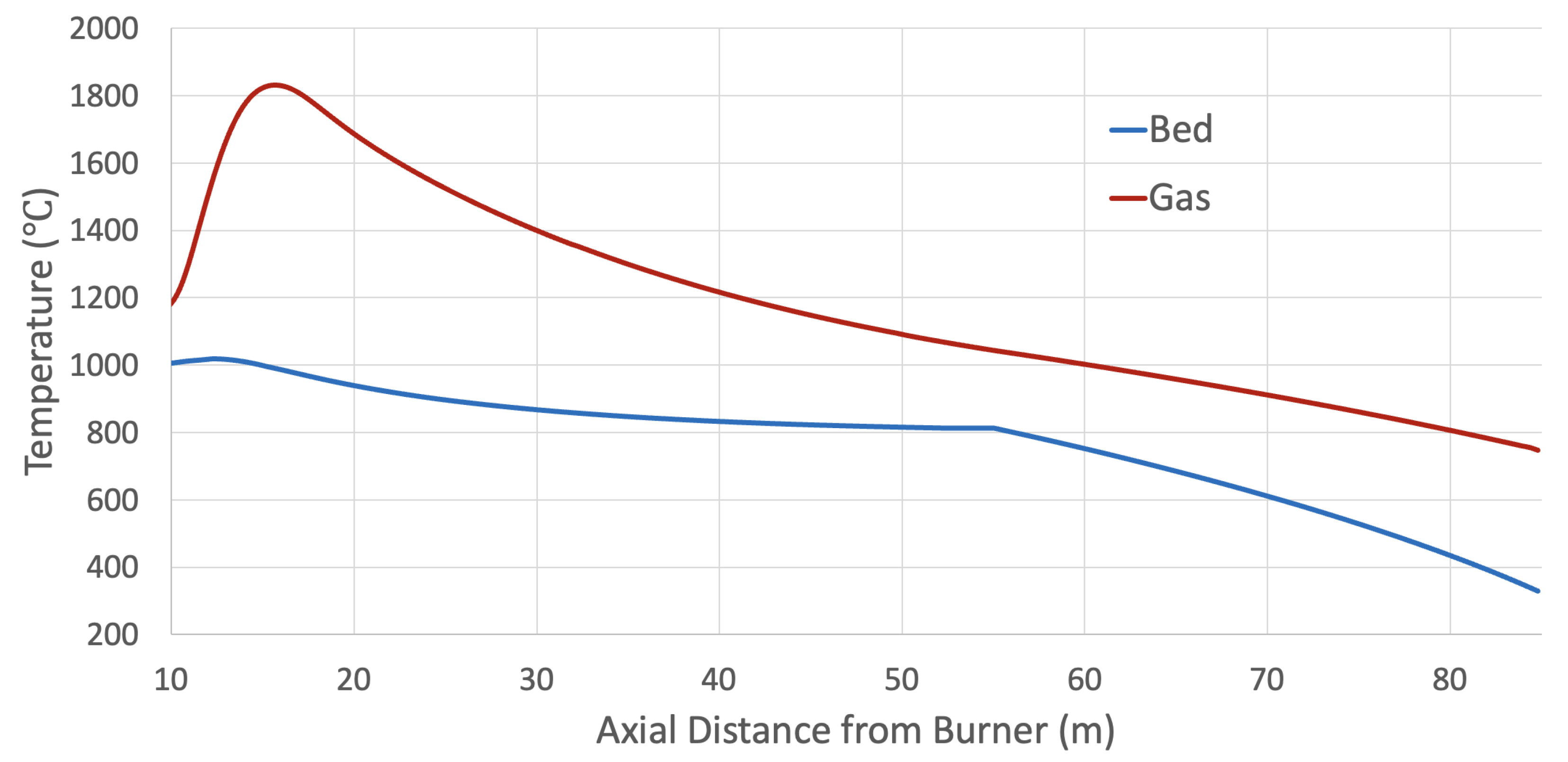
Figure 4 shows the bed and average axial gas temperatures along the dry kiln. A volume average at each cross-section is used to determine the axial gas temperature. The simulated peak average gas temperature is slightly above 1800 °C, which agrees well with previous literature on gas temperatures in rotary lime kilns [50,51]. In addition, since the adiabatic flame temperature of methane is around 2000 °C [52], a peak average gas temperature slightly above 1800 °C is reasonable. Going from left to right, the gas temperature first rises when combustion occurs, reaches a peak 16 m into the kiln (or 10 m from the tip of the burner), then slowly decreases during the rest of the length of the kiln, as heat is transferred from the hot gas to the bed. Going from right to left, the bed enters at 328.5 °C and the temperature increases almost linearly until calcination begins at 57.2 m, where the slope changes due to the calcination reaction, as heat is now absorbed by the reaction instead of heating the bed. The product bed temperature is around 1000 °C, which agrees with other model outputs ranging between 900 °C to 1100 °C [12,17,19,53], which depend on the kiln, the calcination model used, and whether calcination is assumed to be fully complete or not.
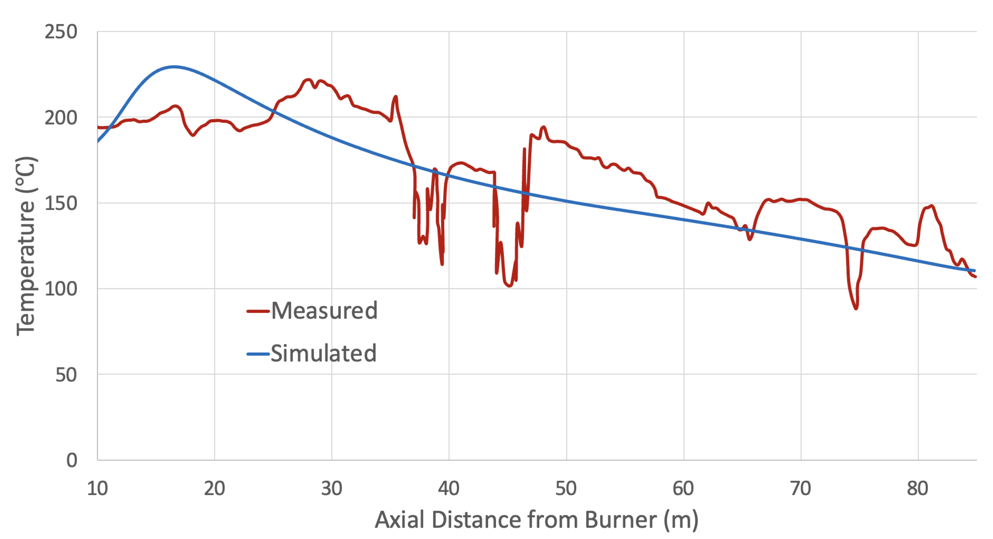
Figure 5 shows the measured and simulated outer shell temperatures along the length of the dry kiln. The shell temperature was measured using a thermal camera and data points were taken at the top of the outer shell. Overall, there is good agreement, which serves to validate the heat loss calculation in the dry kiln model. There is some variability in the measured outer shell temperature, which is due to bearings and other components on the kiln, since the temperature is measured by thermal cameras. In addition, the measured data is also rough and the accuracy of the data is difficult to determine. However, without access to more accurate data, conclusions are drawn with the data available.
Figure 6 shows the bed and average axial gas temperatures along the wet kiln. Comparing Figure 6 to Figure 4, there are some clear differences between the dry and wet kiln. First, the outlet gas temperature for the wet kiln is much lower, 252 °C compared to 750 °C for the dry kiln. There is also a large difference in bed temperature profile, as the wet bed in Figure 6 enters at 25 °C and stays constant at 100 °C while evaporation occurs. In addition, the calcination start location is much closer to the burner in the wet kiln: 43.9 m from the burner instead of 57.2 m in the dry kiln.
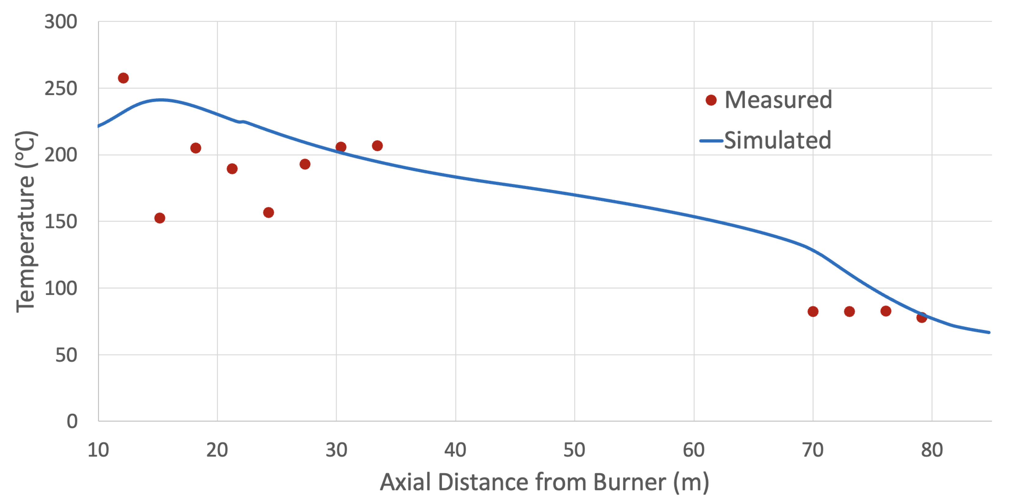
Figure 7 shows the measured and simulated outer shell temperature along the length of the wet kiln. The shell temperature was measured using a thermal camera and data points were taken at the top of the outer shell. The chain section in the kiln is on the far right where the outer shell temperature has a steeper slope. In addition, a slight change in refractory brick can be seen in the simulated data at 23 m from the burner, with a slight drop in temperature in the shell. Otherwise, the good agreement between the simulated and measured outer shell temperature profiles confirm the heat loss calculation in the model.
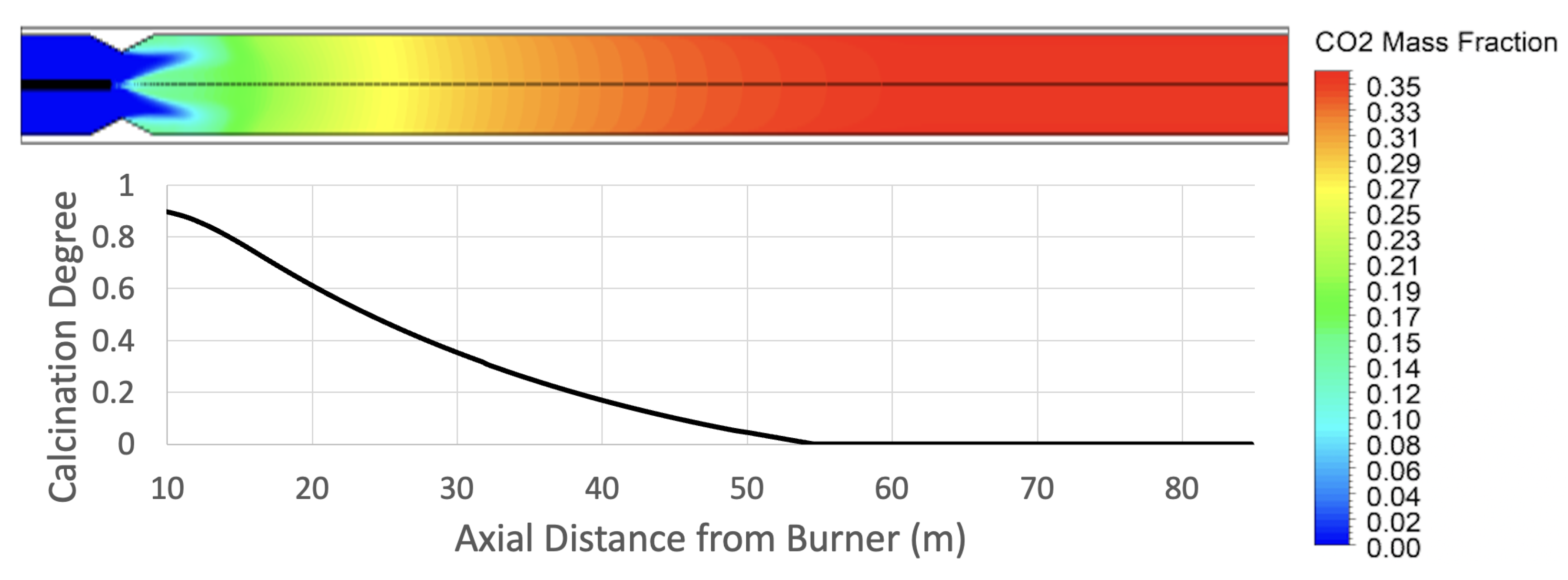
Figure 8 shows the CO2 mass fraction in the dry kiln as well as the degree of calcination along the length of the kiln. The start of calcination occurs at 57.2 m from the burner and continues until the burner. Therefore, the mass fraction of CO2 is at the maximum from the cold end until the start of calcination, and then begins to slowly decrease as the degree of calcination increases. As observed in Equation (29), the difference between the CO2 concentration at the reaction front and in the gas is the driving force in the calcination reaction. Therefore, the mass source of CO2 into the gas from the bed during the calcination reaction, as well as the CO2 gas resulting from combustion, is vital for determining where calcination begins in the kiln.
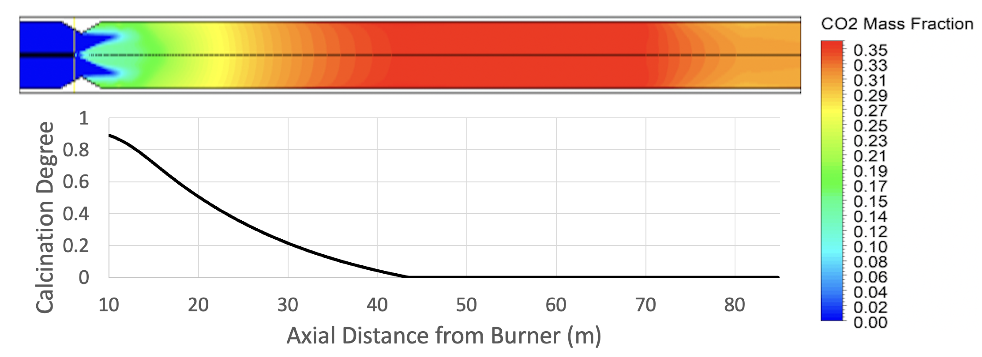
Figure 9 shows the corresponding figure for the wet kiln. The start of calcination in the wet kiln occurs much later, at 43.9 m from the burner, and continues until the burner. However, unlike in the dry kiln, evaporation also occurs in the wet kiln and therefore, the CO2 mass fraction is at the maximum before calcination occurs but decreases in the cold end due to the evaporation of water.
Comparing the dry and wet kiln CO2 mass fractions, both the dry and wet kilns have a maximum CO2 mass fraction of around 0.35. As observed in Figure 8 and Figure 9, CO2 mass and energy transfer from the bed to the gas start at the hot end of the kiln, and this gas is then carried all the way back to the cold end. The amount of CO2 in the gas phase impacts both the properties and temperature of the gas, as well as the heat transfer occurring from the gas to the bed. Therefore, it is clear that proper coupling between the bed and gas for CO2 mass and energy transfer is vital in determining the temperature profiles down the kiln.

3.3. Sensitivity Analysis

A sensitivity analysis was performed to determine the impact that different variables have on the calcination degree and calcination location. From the dry kiln industrial data, Table 4 shows the baseline values that are used for both a regular loading of around 423 t/d of lime and low loading of around 342 t/d of lime. The regular loading had only 0.73% excess O2 in the outlet flue gas, while the low loading had a larger excess O2 of 1.79%, due to the fact that excess air is often increased during lower loading operation to maintain a certain flame shape in the kiln. The other operating conditions or baseline values are roughly the same between the regular and low loading cases.
Table 5 shows the baseline values, which are used for both a regular loading of around 640 t/d of lime mud and low loading of around 377 t/d of lime mud in the wet kiln. The regular loading had a moisture content of 22% whereas the low loading had a moisture content of 19%. The other operating conditions or baseline values are roughly the same between the regular and low loading cases.
Table 6 and Table 7 demonstrate how different variables impact the calcination location and degree for both regular and low loading cases for the dry and wet kilns, respectively. A baseline simulation is first run, and then variables are changed independently by a fixed increment while keeping other variables constant, to determine how the calcination location and degree change compared to the baseline case. The step value of the increment/value column is decided based on a couple of factors. The fuel, excess O2, rotation speed, moisture content, ambient temperature, and particle radius are all based on ranges that are common during operation of the industrial kilns. Feed temperature increment for the dry kiln is estimated based on Equation (9), where −50 °C to −100 °C is chosen. For the wet kiln, since the feed temperature is often around or slightly above room temperature, values around these temperatures are chosen. For the dusting factor, as indicated earlier, dust loss can range between 5% to 20% of the dry lime mud feed rate [6], and so 10% and 20% are chosen to determine the impact of the extent of dusting on the heat transfer results. The chain factor value of 25 is chosen based on the drying length, so an arbitrary increment of ±10 is chosen. The reaction enthalpy for calcination has been reported to range anywhere between 1570 to 1690 kJ/kg [42], while multiple models utilize 1794 kJ/kg [3,10,27,28]. Therefore, the minimum and maximum reported values are chosen as the increment values. Finally, values for the bed emissivity in the literature and previous models have ranged from 0.35 [42,54] to 0.9 [3,10,12,23,28]. In the model, Equation (13) is used to estimate the bed emissivity that depends on temperature, whereas for the increment values, the minimum and maximum values of 0.35 and 0.9 are chosen for comparison.
We define a positive increase in the calcination location to mean that the calcination zone is lengthening and moving towards the cold end of the kiln, and vice versa. Moving forward, any change in calcination location by 1 m or more will be deemed a large impact. A positive percentage increase in the degree of calcination means there is more lime available in the outlet product. The percentage change in degree of calcination is absolute, rather than relative to the baseline value. Moving forward, any change in degree of calcination of 2% or more will be considered a large impact. A positive correlation will refer to an increase in a variable that results in an increase in the length of the calcination zone and degree of calcination, and vice versa.
Of the variables examined in the sensitivity analysis, excess O2, rotation speed, ambient temperature, particle radius, and reaction enthalpy had the smallest impact on the calcination location. Regarding the degree of calcination, excess O2, rotation speed, ambient temperature, and particle radius had the smallest impact. Unlike the calcination location, the reaction enthalpy had a much larger impact on the degree of calcination. It is clearly important to choose the proper reaction enthalpy value for the calcination reaction model. Surprisingly, particle radius has little impact on both the calcination location and degree of calcination. However, the incremental value for the particle radius of ±20% may be lower than what occurs in real kilns during operation, so care should be taken when choosing a proper particle size for calcination.
Of the controllable operating conditions (fuel, excess O2, rotation speed, and moisture content/feed temperature), the fuel rate and the moisture content in the wet kiln, or feed temperature in the dry kiln, have the largest impact on both the calcination location and degree of calcination in the kiln. The increase of 10% in the fuel for the wet kiln results in a larger change to both the calcination location and degree of calcination than the dry kiln; however, this is presumably due to the difference in wall material and heat loss in the two kilns. Feed temperature for the dry kiln and moisture content for the wet kiln also have a large impact on the calcination location and degree of calcination, where the calcination location is impacted more than the degree of calcination. While the feed temperature increment for the wet kiln is small, there is still a relatively large impact on both calcination location and degree, with values ranging from 0.73% to 2.1% change in the length of the calcination zone and 0.22% to 0.79% change in the degree of calcination.
Regarding variables that are not easily controlled by the kiln operator, the dusting factor, chain factor, and bed emissivity also have a large impact on both the calcination location and degree of calcination in the kiln. The values chosen for dusting are based on the possible range of dust loss in the kiln, so 10% and 20% dusting is examined. The dusting factor correlates positively with both the calcination location and degree, as the increase in dusting ultimately increases the thermal conductivity and emissivity of the gas and increases heat transfer to the bed. The dusting factor in the wet kiln has a larger impact on both the calcination location and degree compared to the dry kiln; however, this is likely due to the fact that the dry kiln utilizes more air flow per unit of bed material. Therefore, an increase in dusting in the wet kiln will be a larger total percentage in the gas phase, ultimately having a larger impact on the conductivity and emissivity and increasing the heat transfer to the bed. This model assumes dusting occurs evenly throughout the kiln at a fixed rate; however, in real kilns dusting is a much more complex process, dependent on: particle size, gas velocity, loading rate, and degree of agglomeration [4]. More sophisticated dusting models may be required to determine the impact on the calcination location and degree.
The values chosen for the chain factor are arbitrary, since the chain factor is chosen to obtain a reasonable drying length in the kiln. The chain factor has a positive correlation with both the calcination location and degree, as the chain factor is directly involved with heat transfer to the bed. The chain factor has a slightly larger impact on the regular loading case, likely due to the fact that the gas flow rate in regular loading is higher, which means there is more heat that can be taken from the gas to the bed. The chain factor has a small impact on the degree of calcination, but has a large impact on the calcination location. A more sophisticated model for the chain section may be required to accurately determine the impact of the chain section on the calcination location.
Finally, the values chosen for the bed emissivity are also the minimum and maximum values observed in the literature, as stated earlier. A constant bed emissivity of 0.9 increased the degree of calcination but decreased the calcination location, and vice versa with a constant emissivity of 0.35. This is due to the fact that an increase in emissivity will increase heat transfer by radiation in the hot end of the kiln, increasing the degree of calcination, but ultimately reducing the gas temperature, thereby reducing the calcination location down the kiln. The bed emissivity has a large impact on both the calcination location and degree of calcination. While Equation (13) is used to estimate the bed emissivity, future work may be required to have more confidence in estimating the bed emissivity over a wide range of temperatures.

4. Conclusions

A 2D axisymmetric CFD model is combined with a 1D bed model to simulate heat transfer and calcination within a dry and wet rotary lime kiln. The gas phase is modelled in ANSYS Fluent, where mass and heat sinks are implemented to account for the effects of the bed. The 1D bed model utilizes Kramer’s equation [38] to determine the height and flow rate of the bed material down the kiln. Radiation is modelled using equations developed by Hottel and Sarofim [40]. Conduction and convection is modelled using equations developed by Tscheng and Watkinson [32]. Decomposition is simulated using a shrinking core model and is dependent on the difference in CO2 concentration at the reaction front. The gas and bed models are coupled with two volumetric mass sources, for H2O and CO2, and one volumetric energy source.
Steady-state results for both a dry and wet kiln are in good agreement with mill data, indicating that the model is quite satisfactory. Based on a sensitivity analysis, the location at which calcination begins can shift by multiple meters towards or away from the burner, particularly with fluctuations in fuel to the kiln and moisture content. Interestingly, particle size has a relatively modest effect on the location of calcination in the kiln, and so particle size and particle size distribution may not be too important when modelling calcination. Bed movement likely has a larger impact on heat transfer and therefore calcination, though this is not captured in a 1D bed model. Increased dusting will move the start of calcination further back in the kiln. However, this assumes dusting rises up evenly along the kiln, which is not the case in a real kiln. While a focus has been on the start location of calcination due to the belief that this affects mid-kiln ring formation, the extent of calcination does not necessarily follow directly from the calcination start location. This evaluation is useful for helping to understand the fluctuations in temperature distribution in the kiln and the shift in the starting location of calcination. Further work will involve utilizing the model to study the transient behaviour in rotary lime kilns.

Author Contributions

Conceptualization, M.B. and N.D.; methodology, J.R.; software, J.R.; validation, J.R., M.B. and N.D.; formal analysis, J.R.; investigation, J.R.; resources, N.D.; data curation, J.R.; writing—original draft preparation, J.R.; writing—review and editing, M.B. and N.D.; visualization, J.R.; supervision, M.B. and N.D.; project administration, M.B. and N.D.; All authors have read and agreed to the published version of the manuscript.

Funding

This research received no external funding.

Institutional Review Board Statement

Not applicable.

Informed Consent Statement

Not applicable.

Conflicts of Interest

The authors declare no conflict of interest.

Abbreviations

The following abbreviations are used in this manuscript:
Q ˙ Net heat transfer rate [W]
rRadiative heat transfer
c v Convective heat transfer
c d Conductive heat transfer
s h Kiln outer shell
aAmbient environment
gGas phase
wInner kiln wall
e w Wall exposed to gas phase
c w Wall covered by bed
e b Bed exposed to gas phase
c b Bed covered by wall
c h Chains within the kiln
Sh Sherwood number
Sc Schmidt number
hHeat transfer coefficient [W/m2/K]
kThermal conductivity coefficient [W/m/K]
bBed material
ρ Density [kg/m3]
C p Specific heat capacity [J/kg/K]
α t h Thermal diffusivity [m2/s]
d p Average particle diameter [m]
r p Average particle radius [m]
D e Equivalent diameter of the gas phase [m]
R e g Flow Reynolds number for the gas phase
R e ω Rotational Reynolds number for the gas phase
AHeat transfer area per unit kiln length [m2]
TAbsolute temperature [K]
ϵ Emissivity
α g Absorptivity of the gas phase
e n Emissivity weighting coefficient
a n Absorptivity weighting coefficient
K n Extinction coefficient [1/m]
pPartial pressure of emitting gas species [Pa]
PPressure [Pa]
DDiameter [m]
P r Prandtl number
G r Grasholf number
ν Kinematic viscosity [m2/s]
σ Black body radiation constant [W/m2/K4]
MMolar mass [kg/mol]
RGas constant [J/K/mol]
R i Radius of inner wall [m]
ϕ 0 Central angle of the bed [rad]
ω Kiln rotational velocity [rad/s]
VVelocity [m/s]
fFuel
p a Primary air
s a Secondary air
e s p Electrostatic precipitator
L H 2 O Latent heat vaporization [J/kg]
N p Number of particles
CConcentration [mol/m3]
m ˙ Mass flow rate [kg/s]
o u t Outlet
l a t Latent heat
i n Inner
d e c Decomposition
zAxial position in kiln
L p Path length of a beam through gas [m]
ε Porosity
S m Mass source [kg/s/m3]
S e Energy source [W/m3]
HEnthalpy [J]
fFilling degree
e f f Effective
Φ b Solid volume fraction
Ω Form factor
QVolumetric flow rate [m3/s]
nRotation speed [rev/s]
β Inclination angle from horizontal [rad]
γ Static angle of repose of bed material [rad]
ϕ Central half angle of the bed [rad]
L e b Length of exposed bed [m]
ϕ c h Adjustable chain parameter
R 1 , c Diffusion resistance [s/m]
R 2 , c Boundary layer resistance [s/m]
D e f f Knudsen diffusivity [m2/s]
D k n Knudsen diffusion coefficient [m2/s]
D b i n Binary diffusion coefficient [m2/s]
r ¯ p o r e Mean pore radius [m]
σ a b Characteristic length [m]
Ω D Diffusion collision integral
l a m Laminar
t u r b Turbulent
ϕ a Calcination temperature fraction
ϕ L Heat loss coefficient

References

  1. Davies, P.R.; Norton, M.J.S.; Wilson, D.I.; Davidson, J.F.; Scott, D.M. Gas Flow in Rotary Kilns. Particuology 2010, 8, 613–616. [Google Scholar] [CrossRef]
  2. Boateng, A.A. 1—The Rotary Kiln Evolution and Phenomenon. In Rotary Kilns, 2nd ed.; Boateng, A.A., Ed.; Butterworth-Heinemann: Boston, MA, USA, 2016; pp. 1–11. [Google Scholar] [CrossRef]
  3. Csernyei, C.; Straatman, A.G. Numerical Modeling of a Rotary Cement Kiln with Improvements to Shell Cooling. Int. J. Heat Mass Transf. 2016, 102, 610–621. [Google Scholar] [CrossRef]
  4. Dernegård, H.; Brelid, H.; Theliander, H. Characterization of a Dusting Lime Kiln—A Mill Study. Nord. Pulp Pap. Res. J. 2017, 32, 25–34. [Google Scholar] [CrossRef] [Green Version]
  5. Paul, M.; Tran, H.N.; Kuhn, D.C.S.; Faulkner, R. Investigation of Nodule Formation in Lime Kilns Using Batch Kilns. Mining Metall. Explor. 2006, 23, 219–225. [Google Scholar] [CrossRef]
  6. Tran, H. Lime Kiln Chemistry and Effects on Kiln Operations. In TAPPI Kraft Recovery Course; TAPPI PRESS: Atlanta, GA, USA, 2007. [Google Scholar]
  7. Tran, H.; Mao, X.; Barham, D. Mechanisms of Ringing Formation in Lime Kilns. J. Pulp Pap. Sci. 1993, 19, J167–J175. [Google Scholar]
  8. Kalaie, A.; Li, S.; Wang, Y.; Wang, X. A Multi-Model Fusion Soft Sensor Modelling Method and Its Application in Rotary Kiln Calcination Zone Temperature Prediction. Trans. Inst. Meas. Control 2015, 38, 110–124. [Google Scholar] [CrossRef]
  9. Gonzalez, H.; Zarate Evers, C.; Alviso, D.; Rolon, J. Numerical Study of a Rotary Kiln. Case of an Industrial Plant in Paraguay. In Proceedings of the Brazilian Congress of Thermal Sciences and Engineering, Belem, Brazil, 10–13 November 2016. [Google Scholar] [CrossRef]
  10. Mujumdar, K.; Ranade, V. Simulation of Rotary Cement Kilns Using a One-Dimensional Model. Chem. Eng. Res. Des. 2006, 84, 165–177. [Google Scholar] [CrossRef]
  11. Gaurav, G.K.; Khanam, S. Computational Fluid Dynamics Analysis of Sponge Iron Rotary Kiln. Case Stud. Therm. Eng. 2017, 9, 14–27. [Google Scholar] [CrossRef] [Green Version]
  12. Agrawal, A.; Ghoshdastidar, P. Computer Simulation of Heat Transfer in a Rotary Lime Kiln. J. Therm. Sci. Eng. Appl. 2018, 10, 031008-1. [Google Scholar] [CrossRef]
  13. Akgun, F. Investigaton of Energy Saving and NOx Reduction Possibilities in a Rotary Cement Kiln. Int. J. Energy Res. 2003, 27, 455–465. [Google Scholar] [CrossRef]
  14. Alyaser, A.H. Fluid Flow and Combustion in Rotary Kiln. Ph.D. Thesis, University of British Columbia, Vancouver, BC, Canada, 1998. [Google Scholar] [CrossRef]
  15. Ariyaratne, W.K.H.; Malagalage, A.; Melaaen, M.C.; Tokheim, L.A. CFD Modelling of Meat and Bone Meal Combustion in a Cement Rotary Kiln—Investigation of Fuel Particle Size and Fuel Feeding Position Impacts. Chem. Eng. Sci. 2015, 123, 596–608. [Google Scholar] [CrossRef]
  16. Barr, P.V.; Brimacombe, J.K.; Watkinson, A.P. A Heat-Transfer Model for the Rotary Kiln: Part II. Development of the Cross-Section Model. Metall. Mater. Trans. B 1989, 20, 403–419. [Google Scholar] [CrossRef]
  17. Barr, P.V. Heat Transfer Processes in Rotary Kilns. Ph.D. Thesis, University of British Columbia, Vancouver, BC, Canada, 1986. [Google Scholar] [CrossRef]
  18. Georgallis, M. Mathematical Modelling of Lime Kilns. Ph.D. Thesis, University of British Columbia, Vancouver, BC, Canada, 2004. [Google Scholar] [CrossRef]
  19. Georgallis, M.; Nowak, P.; Salcudean, M.; Gartshore, I.S. Modelling the Rotary Lime Kiln. Can. J. Chem. Eng. 2005, 83, 212–223. [Google Scholar] [CrossRef]
  20. Gorog, J.P.; Adams, T.N.; Brimacombe, J.K. Heat Transfer from Flames in a Rotary Kiln. Metall. Trans. B 1983, 14, 411–424. [Google Scholar] [CrossRef]
  21. Gorog, J.P.; Brimacombe, J.K.; Adams, T.N. Radiative Heat Transfer in Rotary Kilns. Metall. Trans. B 1981, 12, 55–70. [Google Scholar] [CrossRef]
  22. Gunnarsson, A.; Andersson, K.; Adams, B.R.; Fredriksson, C. Full-Scale 3D-modelling of the Radiative Heat Transfer in Rotary Kilns with a Present Bed Material. Int. J. Heat Mass Transf. 2020, 147, 118924. [Google Scholar] [CrossRef]
  23. Hanein, T.; Glasser, F.P.; Bannerman, M.N. One-Dimensional Steady-State Thermal Model for Rotary Kilns Used in the Manufacture of Cement. Adv. Appl. Ceram. 2017, 116, 207–215. [Google Scholar] [CrossRef]
  24. Li, S.Q.; Ma, L.B.; Wan, W.; Yao, Q. A Mathematical Model of Heat Transfer in a Rotary Kiln Thermo-Reactor. Chem. Eng. Technol. 2005, 28, 1480–1489. [Google Scholar] [CrossRef]
  25. Liu, H.; Yin, H.; Zhang, M.; Xie, M.; Xi, X. Numerical Simulation of Particle Motion and Heat Transfer in a Rotary Kiln. Powder Technol. 2016, 287, 239–247. [Google Scholar] [CrossRef]
  26. Macphee, J. CFD Modelling of a Rotary Lime Kiln. Master’s Thesis, University of Canterbury, Christchurch, New Zealand, 2010. [Google Scholar]
  27. Mintus, F.; Hamel, S.; Krumm, W. Wet Process Rotary Cement Kilns: Modeling and Simulation. Clean Technol. Environ. Policy 2006, 8, 112–122. [Google Scholar] [CrossRef]
  28. Mujumdar, K.S.; Ranade, V.V. CFD Modeling of Rotary Cement Kilns. Asia-Pac. J. Chem. Eng. 2008, 3, 106–118. [Google Scholar] [CrossRef]
  29. Shi, D.; Vargas, W.L.; McCarthy, J.J. Heat Transfer in Rotary Kilns with Interstitial Gases. Chem. Eng. Sci. 2008, 63, 4506–4516. [Google Scholar] [CrossRef]
  30. Spang, H.A. A Dynamic Model of a Cement Kiln. Automatica 1972, 8, 309–323. [Google Scholar] [CrossRef]
  31. Tao, L.; Nordgren, D.; Blom, R. Development of a Three-Dimensional CFD Model for Rotary Lime Kilns; Technical Report; Värmeforsk ServiceAB: Stockholm, Sweden, 2010. [Google Scholar]
  32. Tscheng, S.H.; Watkinson, A.P. Convective Heat Transfer in a Rotary Kiln. Can. J. Chem. Eng. 1979, 57, 433–443. [Google Scholar] [CrossRef] [Green Version]
  33. Watkinson, A.P.; Brimacombe, J.K. Limestone Calcination in a Rotary Kiln. Metall. Trans. B 1982, 13, 369–378. [Google Scholar] [CrossRef]
  34. Ginsberg, T.; Modigell, M. Dynamic Modelling of a Rotary Kiln for Calcination of Titanium Dioxide White Pigment. Comput. Chem. Eng. 2011, 35, 2437–2446. [Google Scholar] [CrossRef]
  35. Gareau, P.R. A CFD Study of the Effects of Rings on Flow and Temperature in Lime Kilns. Master’s Thesis, University of Toronto, Toronto, ON, Canada, 2020. [Google Scholar]
  36. ANSYS. ANSYS FLUENT 12.0 User’s Guide. 2009. Available online: https://www.afs.enea.it/project/neptunius/docs/fluent/html/ug/main_pre.htm (accessed on 11 September 2021).
  37. Hart, P.W.; Hanson, G.M., 3rd; Manning, R.P. Lime Kilns and Recausticizing: The Forgotten Part of a Kraft Mill; Technical Association of the Pulp & Paper Industry: Peachtree Corners, GA, USA, 2021. [Google Scholar]
  38. Kramers, H.; Croockewit, P. The Passage of Granular Solids through Inclined Rotary Kilns. Chem. Eng. Sci. 1952, 1, 259–265. [Google Scholar] [CrossRef]
  39. Spurling, R.J.; Davidson, J.F.; Scott, D.M. The Transient Response of Granular Flows in an Inclined Rotating Cylinder. Chem. Eng. Res. Des. 2001, 79, 51–61. [Google Scholar] [CrossRef]
  40. Hottel, H.; Sarofim, A. Radiative Transfer. AIChE J. 1969, 15, 794–796. [Google Scholar] [CrossRef]
  41. Vangaever, S.; Van Thielen, J.; Hood, J.; Olver, J.; Honnerovà, P.; Heynderickx, G.J.; Van Geem, K.M. The Effect of Refractory Wall Emissivity on the Energy Efficiency of a Gas-Fired Steam Cracking Pilot Unit. Materials 2021, 14, 880. [Google Scholar] [CrossRef]
  42. Sandaka, G. Calcination Behavior of Lumpy Limestones from Different Origins. Ph.D. Thesis, Otto von Guericke University Magdeburg, Magdeburg, Germany, 2016. [Google Scholar]
  43. Bluhm-Drenhaus, T.; Simsek, E.; Wirtz, S.; Scherer, V. A Coupled Fluid Dynamic-Discrete Element Simulation of Heat and Mass Transfer in a Lime Shaft Kiln. Chem. Eng. Sci. 2010, 65, 2821–2834. [Google Scholar] [CrossRef]
  44. Maya, J.C.; Chejne, F.; Gómez, C.A.; Bhatia, S.K. Effect of the CaO Sintering on the Calcination Rate of CaCO3 under Atmospheres Containing CO2. AIChE J. 2018, 64, 3638–3648. [Google Scholar] [CrossRef]
  45. Reid, R.C.; Prausnitz, J.M.; Poling, B.E. The Properties of Gases and Liquids, 4th ed.; McGraw Hill Book Co.: New York, NY, USA, 1987. [Google Scholar]
  46. Everest Interscience. Emissivity of Total Radiation for Various Metals; Everest Interscience: Tucson, AZ, USA, 2021; Available online: http://everestinterscience.com/info/emissivitytable.htm (accessed on 11 February 2021).
  47. Harbison Walker. Handbook of Refractory Practice; Harbison Walker: Pittsburgh, PA, USA, 2021; Available online: https://www.mha-net.org/docs/Harbison%20Walker%202005%20Handbook.pdf (accessed on 11 February 2021).
  48. Kodur, V.; Kand, S.; Khaliq, W. Effect of Temperature on Thermal and Mechanical Properties of Steel Bolts. J. Mater. Civ. Eng. 2012, 24, 765–774. [Google Scholar] [CrossRef]
  49. Weather Underground. Weather Underground; Weather Underground: San Francisco, CA, USA; Available online: https://www.wunderground.com/ (accessed on 12 July 2021).
  50. Shahin, H.; Hassanpour, S.; Saboonchi, A. Thermal Energy Analysis of a Lime Production Process: Rotary Kiln, Preheater and Cooler. Energy Convers. Manag. 2016, 114, 110–121. [Google Scholar] [CrossRef]
  51. Elattar, H.F.; Specht, E.; Fouda, A.; Bin-Mahfouz, A.S. Study of Parameters Influencing Fluid Flow and Wall Hot Spots in Rotary Kilns Using CFD. Can. J. Chem. Eng. 2016, 94, 355–367. [Google Scholar] [CrossRef]
  52. Pupo, R. Adiabatic Flame Temperature for Combustion of Methane II. Undergrad. J. Math. Model. One + Two 2013, 5, 1. [Google Scholar] [CrossRef]
  53. Fardadi, M. Modeling Dust Formation in Lime Kilns. Ph.D. Thesis, University of Toronto, Toronto, ON, Canada, 2010. [Google Scholar]
  54. Moldenhauer, A.; Bauer, W.; Specht, E.; Herz, F. Thermophysical Properties of Lime as a Function of Origin (Part 3): Emissivity. ZKG Int. 2016, 69, 58–62. [Google Scholar]
Figure 1. Rotary kiln with counter flow of the gas and bed.
Processes 10 01516 g001
Figure 2. Mesh near the burner and dam of the kiln.
Processes 10 01516 g002
Figure 3. Burner geometry.
Processes 10 01516 g003
Figure 4. Simulated bed and average axial gas temperature for a dry kiln.
Processes 10 01516 g004
Figure 5. Measured and simulated dry kiln outer shell temperature.
Processes 10 01516 g005
Figure 6. Simulated bed and average axial gas temperatures for a wet kiln.
Processes 10 01516 g006
Figure 7. Measured and simulated wet kiln outer shell temperature.
Processes 10 01516 g007
Figure 8. CO2 mass fraction and degree of calcination for a dry kiln.
Processes 10 01516 g008
Figure 9. CO2 mass fraction and degree of calcination for a wet kiln.
Processes 10 01516 g009
Table 1. Dry and wet kiln dimensions.
Dry KilnWet Kiln
VariableValueUnitsValueUnits
Total Length85m85m
Outer Diameter3.75m3.2m
Refractory Thickness0.2286m0.2159m
Shell Thickness0.0254m0.0191m
Table 2. Dry and wet kiln steady-state simulation values.
Dry KilnWet Kiln
VariableValueUnitsValueUnits
Dry Loading9.9kg/s7.2kg/s
Fuel Flow0.68kg/s0.44kg/s
Primary Air Flow2.9kg/s0.54kg/s
Secondary Air Flow9.0kg/s7.5kg/s
Excess O20.6%1.0%
Rotation Speed1.4RPM1.0RPM
Feed Temperature328.5°C25°C
Moisture Content--20%
Secondary Air Temperature286.2°C282.8°C
Ambient Temperature−11.1°C34.2°C
Particle Radius10mm10mm
Table 3. Dry and wet kiln steady-state simulated vs measured values.
SimulatedMeasuredUnits
VariableDry Kiln
Outlet Gas Temperature750750°C
Residual Carbonates-1.0%
Lime Availability90.9-%
Wet Kiln
Outlet Gas Temperature252250°C
Outlet Bed Temperature932905°C
Residual Carbonates-3.0%
Lime Availability85.0-%
Table 4. Dry kiln baseline values.
Dry Kiln
VariableRegular Loading ValueLow Loading
Value
Unit
Dry Loading423342t/d Lime
Fuel Flow0.680.55kg/s
Excess O20.731.8%
Rotation Speed1.51.5RPM
Feed Temperature327327°C
Ambient Temperature12.213.9°C
Particle Radius1010mm
Dusting Factor0.050.05-
Reaction Enthalpy16301630kJ/kg
Bed EmissivityEquation (13)Equation (13)-
Table 5. Wet kiln baseline values.
Wet Kiln
VariableRegular Loading ValueLow Loading
Value
Unit
Dry Loading640500t/d Lime Mud
Fuel Flow0.460.39kg/s
Excess O21.01.0%
Rotation Speed1.01.0RPM
Moisture Content0.220.19%
Feed Temperature2525°C
Ambient Temperature1010°C
Particle Radius1010mm
Dusting Factor0.050.05-
Chain Factor2525-
Reaction Enthalpy16301630kJ/kg
Bed EmissivityEquation (13)Equation (13)-
Table 6. Regular and low loading comparison for dry kiln.
Dry Kiln
Regular LoadingLow Loading
VariableIncrement/ValueCalcination Location (m)Calcination Degree (%)Calcination Location (m)Calcination Degree (%)
BaselineBaseline56.592.156.190.3
Fuel+10%+1.5+5.7+1.6+6.3
−10%−1.8−6.8−1.9−6.9
Excess O2+50%+0.085−1.4+0.29−3.6
−50%−0.12+1.1−0.24+2.7
Rotation+20%+0.19−1.2+0.22−0.98
Speed−20%−0.26+1.3−0.27+1.2
Feed−50 °C−1.1−0.79−0.90−0.60
Temperature−100 °C−1.1−1.3−0.95−1.0
Ambient+20 °C+0.073+0.73+0.12+0.87
Temperature−20 °C−0.12−0.91−0.11−0.92
Particle+20%+0.18−1.1+0.25−0.93
Radius−20%−0.25+0.96−0.29+1.0
Dusting0.1+0.29+1.1+0.30+1.1
Factor0.2+0.85+3.2+0.79+3.0
Reaction1794 kJ/kg−0.39−6.7−0.37−6.7
Enthalpy1570 kJ/kg+0.12+2.5+0.19+2.6
Bed0.9−0.68+2.5−0.62+2.3
Emissivity0.35+0.35−3.3+0.40−2.9
Table 7. Regular and low loading comparison for wet kiln.
Wet Kiln
Regular LoadingLow Loading
VariableIncrement/ValueCalcination Location (m)Calcination Degree (%)Calcination Location (m)Calcination Degree (%)
BaselineBaseline42.788.442.489.5
Fuel+10%+3.4+7.9+3.9+8.2
−10%−4.1−9.1−4.2−9.1
Excess O2+50%+0.32−1.6+0.59−1.3
−50%−0.56+1.3−0.33+1.4
Rotation+20%+0.17-1.1+0.23−0.99
Speed−20%−0.13+1.5−0.31+1.3
Moisture+40%−4.6−4.9−4.0−3.7
Content−40%+4.1+3.5+3.9+2.7
Feed+15 °C+0.31+0.22+0.51+0.39
Temperature+30 °C+0.90+0.79+0.72+0.60
Ambient+20 °C−0.021+0.081+0.024+0.13
Temperature−20 °C+0.021−0.081−0.019−0.13
Particle+20%+0.32−0.75+0.33−0.76
Radius−20%−0.40+0.79−0.39+0.88
Dusting0.1+0.47+1.5+0.39+1.2
Factor0.2+1.5+4.2+1.2+3.4
Chain15−1.8−1.9−1.6−-1.3
Factor35+2.2+2.0+1.6+1.3
Reaction1794 kJ/kg−0.39−7.0−0.51−6.9
Enthalpy1570 kJ/kg+0.18+2.7+0.18+2.7
Bed0.9−0.98+2.0−0.84+1.9
Emissivity0.35+0.51−2.9+0.93−2.2
Publisher’s Note: MDPI stays neutral with regard to jurisdictional claims in published maps and institutional affiliations.

