1. Introduction
Modeling the dynamics of a sliding droplet on a vertical surface excited by external forces such as gravity, pressure gradient, and the attractive/repulsive wetting molecular forces at the fluid–solid contact point can help to describe the processes of many practical applications such as inkjet printing [
1], enhanced oil recovery [
2], and film coating [
3].
However, most substrate surfaces are not perfectly smooth and present irregularities that can dramatically change the dynamic behavior of the sliding droplet. Furthermore, some applications require engineered surfaces corrugated with periodic groove ridges to enhance their wettability properties [
4]. Therefore, it is essential to understand how the wettability of such grooved-ridged surfaces is affected by their primary dimensions and spacing. Hence, this study examines the droplet movement and deformation on a grooved-ridged vertical surface under varying wettability conditions.
Two primary states, namely Cassie–Baxter [
5] and Wenzel [
6], have been historically identified on grooved-ridged surfaces. Both are produced by minimizing the system’s free energy under various conditions. The droplet contact line advances over the surface in the Wenzel state, filling the substrate groove voids between the ridges. The surface roughness enlarges the effective surface area of the wall, and the contact angle measured on a flat surface is adjusted according to [
5]:
where the surface roughness is accounted for by
r, which is generally more than 1. Thus, Equation (1) illustrates how the surface roughness affects the apparent wettability of a given surface under the presence of a sessile droplet in the Wenzel state. On the other hand, Cassie and Baxter [
5] suggested a correlation between the apparent contact angle and surface roughness when the droplet does not fill the cavities. Their proposal was based on the hypothesis that the droplet constantly rests on top of the roughness. The apparent contact angle is determined by Equation (2) [
6]:
where
is the fraction of the area of the surface moistened with a drop.
Droplets in the Cassie–Baxter and Wenzel states are ubiquitous in nature and engineering applications. For example, Cassie–Baxter droplets are frequently spotted on hydrophobic surfaces such as butterfly wings and lotus leaves [
7]. Surfaces with the Cassie–Baxter state have numerous desirable qualities, including low adhesion, water repellency, and high droplet mobility, which may be utilized to minimize drag in microfluidic devices, fuel cell chips, and self-cleaning surfaces [
8]. On the other hand, irregularities on hydrophilic surfaces increase their capacity to entrain droplets in the Wenzel state, which is ideal for applications requiring good solid–liquid contacts, such as heat control microfluidics and pesticide retention on plants [
9]. Therefore, it is necessary to study the behavior of drops in the Cassie–Baxter, and Wenzel states to maximize the benefits of rough surfaces in engineering applications. Numerical simulations can help us design microfluidic grooved-ridged surfaces by controlling the different wettability conditions under horizontal and vertical configurations, provided the numerical model can capture the rich physics behind the interface motion and deformation of the sliding droplet.
The Lattice Boltzmann method (LBM) has emerged as a suitable numerical tool for modeling fluid flows. The basic idea behind the Lattice Boltzmann technique is to build simpler kinetic models that include the critical physics of mesoscopic or microscopic processes so that the macroscopic averaged attributes also reproduce macroscopic continuum equations. In addition, the straightforward implementation of boundary conditions, programming simplicity, and the ability to incorporate microscopic interactions are advantages that the LBM provides [
10]. The LBM has been used in previous studies of multiphase and multicomponent flows in porous media and single domains [
11,
12,
13,
14,
15]. For example, Suo, Liu, and Gan [
16] studied the transport and spreading of droplets through porous media. Wang and Wang [
17] successfully investigated the movement of a droplet along a filament under the effect of gravity force. Additionally, Chen et al. [
18] studied the spreading of a 3D droplet on an inclined wall using the LBM with a single-component multiphase pseudopotential model. Bhardwaj and Dalal [
19] did a mesoscopic analysis of 3D droplet displacement on wetted grooved wall microchannel under the gravity influence. Hyväluoma et al. [
20] analyzed a 3D droplet sliding on a micro-grooved wall under various angles, utilizing SC-LBM. However, the variation of geometric parameters of the wall and modeling the detachment were not considered. Zhou et al. [
21] performed a similar 2D study featuring a flow model in a channel lined with grooves. Vrancken et al. [
22] studied the reversible transition of a droplet between Cassie–Baxter and Wenzel states using the free-energy LBM model with experimental validation, but the droplet detachment was not considered. Droplet detachment was considered instead by Kang, Zhang and Chen [
23] in a similar study featuring 3D SC-LBM, analyzing the effect of contact angle, but only with smooth walls. Wang, Deng and Zhang [
24] developed a model of droplet detachment from a grooved surface, but in a downward-horizontal orientation, with a droplet dripping without controlling the Bond number. Despite the 3D approach being a more realistic depiction of a physical system, 2D models have proven to be a valid alternative in preliminary analyses successfully describing essential features of droplet dynamics interacting with solid surfaces.
Thus, in the present study, we used a 2D SC-LBM, following our earlier work [
25], to study droplet spreading on a horizontal grooved surface and, for the first time to our knowledge, the droplet detachment from a vertical grooved surface as a case of practical interest. Cassie–Baxter and Wenzel’s states were explored, primarily focusing on observing the contact angle dynamics under the interaction of solid–fluid adhesion forces, driving body force intensity, and fluid–fluid surface tension.
2. Methodology
The LBM formulation considers the fluid as a set of fictitious particle packages interacting and moving according to probability distribution functions. The particles collide instantaneously and stream in a predetermined pattern and speed to neighboring nodes every time step in a Cartesian grid (i.e., a lattice). A single probability distribution function describes each fluid particle’s physical condition at a particular time step in a given node. After the particles collide, the system transits to reach its local equilibrium condition in a relaxation time before streaming. As a result, every probability distribution function in the model is associated with a fluid component and a given streaming velocity vector, governed by the following Lattice Boltzmann Equation (3):
where
represents the particle’s probability distribution function for the fluid component “α” in the “
ith” direction,
is the equilibrium distribution function in the corresponding lattice velocity direction and fluid component,
is the microscopic velocity in the i
th direction,
is the time-step, and τ is the relaxation time.
The collision operator on the right side of Equation (3) is based on the Bhatnagar–Gross–Krook (BGK) approximation [
10], and the streaming step is on the left side. Because the collision is only local to a single node, the LBM is suitable for massively parallel calculations on many CPU or GP-GPU systems. On the other hand, streaming provides data transfer from one node to the following [
26]. The dimensionless relaxation time of component “α”,
, is connected with its kinematic viscosity by
=
(
−0.5
).
In the present work, the droplet analysis will be undertaken as a fluid immersed in another fluid phase. The proposed two-component multiphase model is the Shan-Chen (SC) LBM with a D2Q9 lattice scheme, i.e., two-dimensional nine-velocity directions.
For the current suggested model, the equilibrium distribution function is:
where
u and
ρ represent the macroscopic velocity and density, and
designates the weighting factor. The weighting factor
for
i = 0 is 4/9, while
i = 1, 2, 3, and 4 is 1/9, and
i = 5, 6, 7, and 8 is 1/36. The moments of the probability distribution functions are shown in Equations (5) and (6) to calculate the density
and momentum density
.
The cohesive force between the two components is given by the Equation (7) [
27]:
where
represents the inter-particle interaction strength, either positive or negative depending on the nature of the resulting force, i.e., attraction or repulsion, respectively. If the threshold point of interaction strength is surpassed, phase separation occurs spontaneously. The behavior of a non-ideal fluid is represented using an interaction parameter termed effective mass, which is meant to replicate the function of a Lennard-Jones potential [
28]. The density plays this role in Equation (7).
Moreover, Equation (8) defines the adhesive force between the solid substrate and the fluid [
29]:
where
s = 0 denotes a fluid node,
s = 1 denotes a solid substrate, and
is the wettability factor, also known as the solid–fluid interaction parameter, which indicates the strength of the interaction between the solid and fluid. A non-wetting fluid–surface contact has a positive
, while a wetting fluid–surface interaction has a negative
[
26]. A body force is used to create a flow in vertical cases:
where
g is body force per unit mass. Throughout every spatial point on the grid nodes, the forces stated above operate on the respective fluid component.
The effect of forces is accounted for by calculating the velocity under the influence of forces
, as shown in Equation (10), a component of Equation (4).
3. Verification and Validation of the LBM Model
The present study continues our previous work [
25], where the earlier described LBM model was validated on a 2D sessile droplet and a two-fluid stratified Poiseuille flow. The present study further analyzes the droplet spreading on a roughened surface represented by horizontal and vertical groove-ridge patterned surfaces. Firstly, the static contact angle on the groove-ridge surface was measured and compared with the theoretical contact angle determined by Equations (1) and (2) to prove the validity of the LBM code used in the study. The equivalent surface roughness
r was defined by
; where
w and
h are the ridge width and height, and
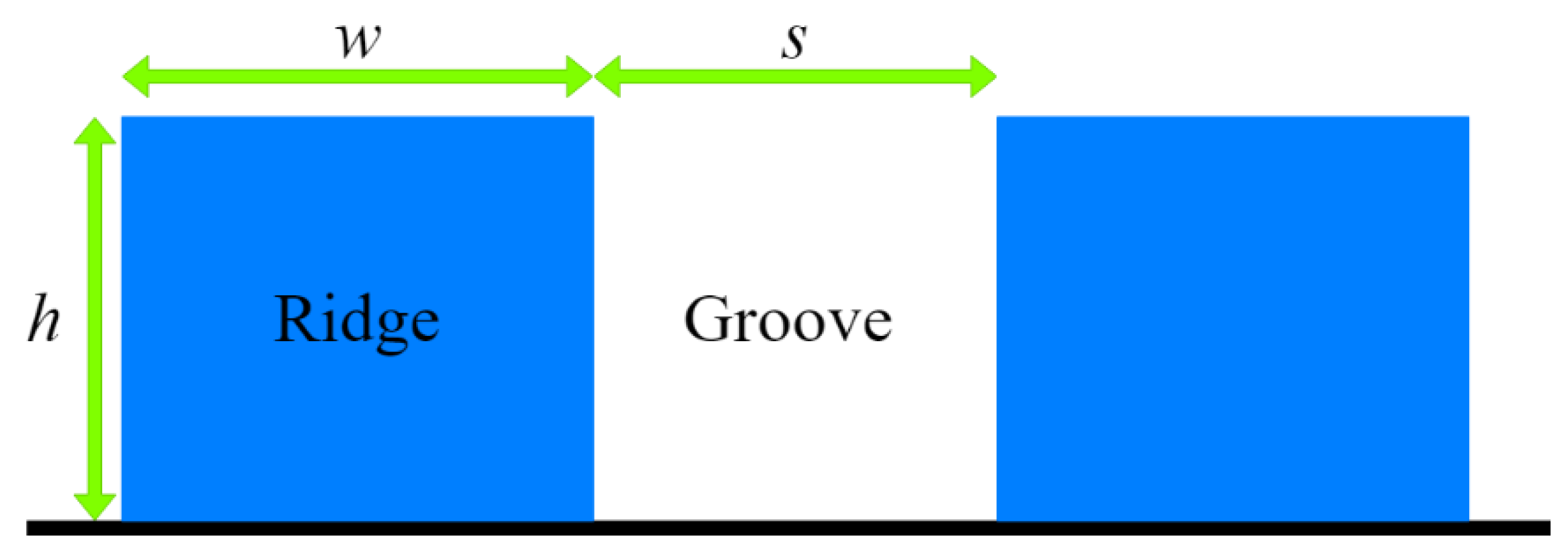
s denotes the spacing between the ridges, as shown in
Figure 1. The static contact angle is prescribed for the flat surface, as in our previous work [
25]. The solid fraction
in Equation (2) was determined by
. As explained in the next section, changing the groove-ridge dimensions triggered the Cassie–Baxter and Wenzel wetting states.
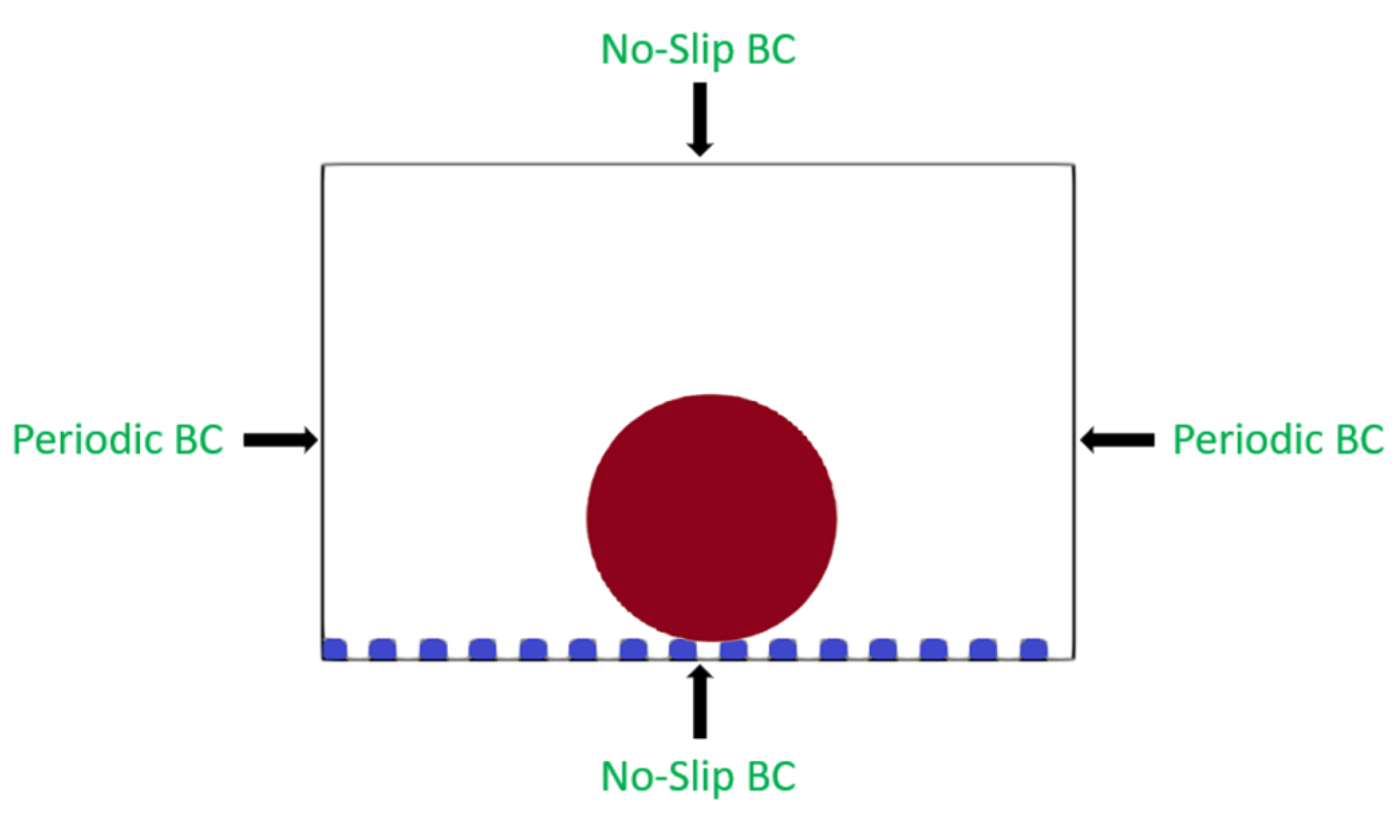
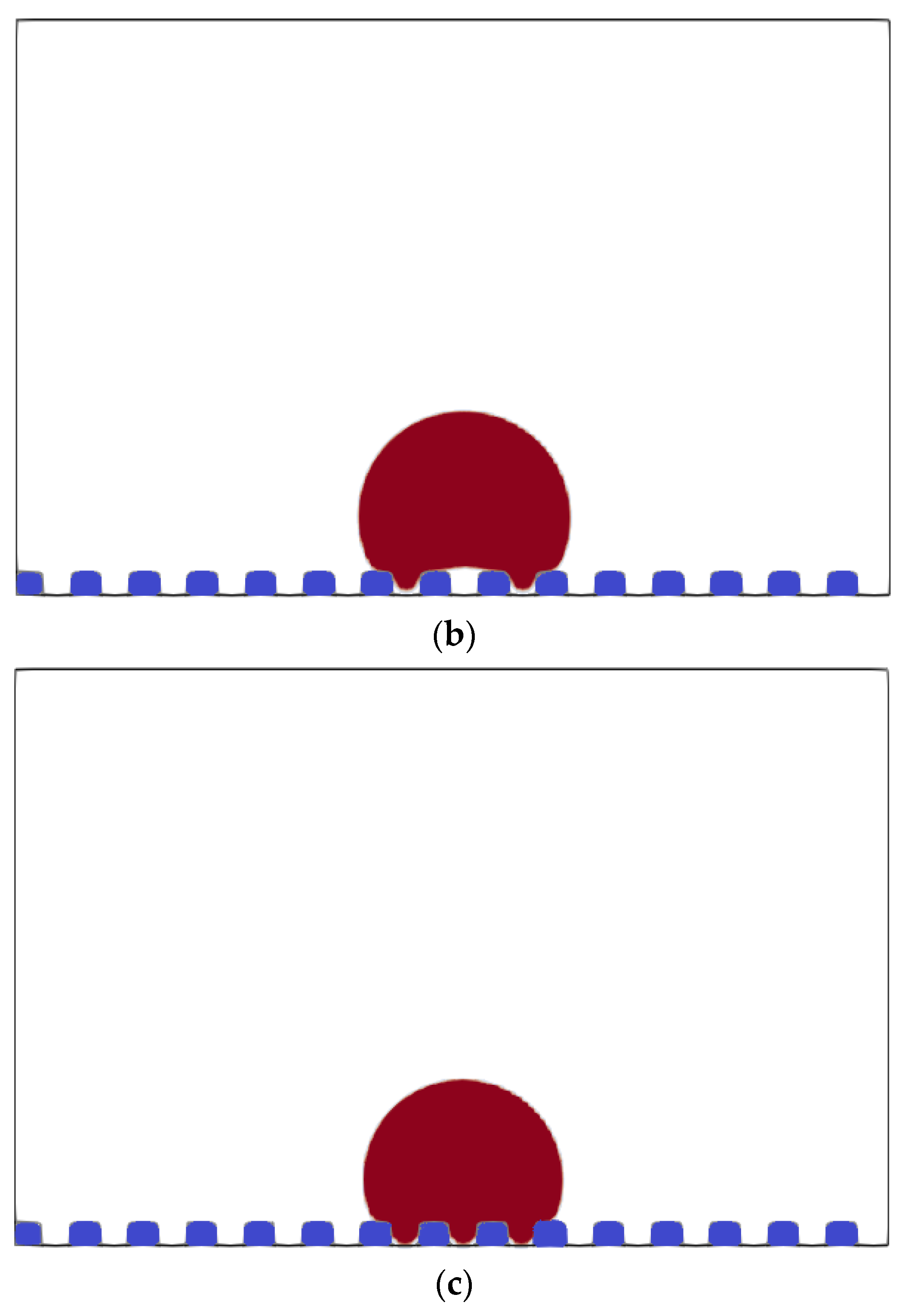
The horizontal grooved-ridged surface is firstly studied without including gravitational effects. As indicated in our previous work [
25], a 2D liquid droplet is placed at the chamber’s center, surrounded by an immiscible background fluid. The domain geometry, initial, and boundary conditions are shown in
Figure 2, with the weightless droplet in its initial state. Hence, a droplet with a radius of 20 lattice units (lu) was placed in the middle between two contiguous ridges. The no-slip boundary condition (BC) is imposed on the top and bottom walls, whereas periodic BCs are prescribed on the left and right sides of the domain. The no-slip boundary condition is applied by reversing the distribution function on each wall node
,
, where
j is the direction opposite to the initial direction
i, so
. The periodic boundary condition is applied by translating the values of the probability distribution function at the boundary node
to the opposing side node
, preserving the directions,
.
The size of the initial computational domain is 151 × 101 lu
2. This mesh configuration was chosen as an initial set-up because it was used in our previous work [
25] for correctly reproducing static contact angles.
The height (
h) and width (
w) of the ridges, and the spacing (
s) between the two ridges, were varied to observe the droplet spreading over the ribbed surface to depict either the Wenzel and Cassie–Baxter states. Geometrical considerations were used to determine the droplet contact angle once it reached equilibrium, as reported in [
25]. The SC-LBM model showed its excellent capability in recreating these classical hydrophilic or hydrophobic states.
The first set of geometrical parameters used was w = h = s = 5 lu, with a roughness of r = 1.44. Wenzel’s wettability state was attained from this initial simulation. For the initial mesh, Wenzel’s state contact angle obtained from the numerical simulation is 69.3°, close to the theoretical value of 69.6° calculated via Equation (1).
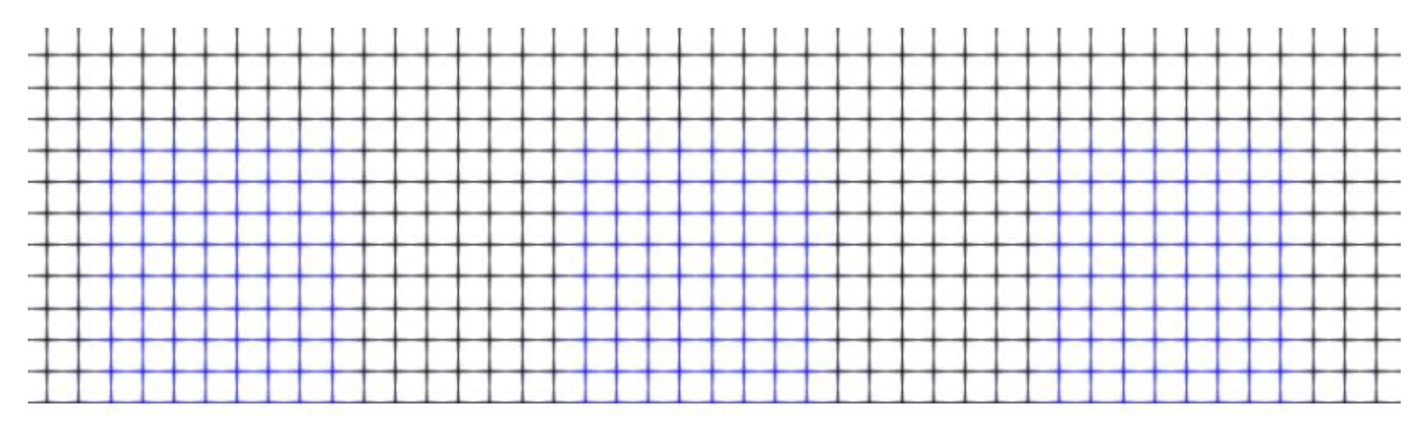
The required verification of the domain discretization was conducted before validating the numerical findings using a progressive grid refinement method. The grid highlighted on top of the grooved wall geometry is shown in
Figure 3. The domain height (y-direction) was discretized with a fixed medium resolution of 101 lu-grid because the vertical grid size was not expected to affect Wenzel’s contact angle, as it greatly depends on the x-discretization. As a result, the horizontal grid size (x-direction) was the focus of the grid verification. The domain’s x-grid was refined by 33% twice (see
Table 1). The contact angle at the Wenzel state between the first and second grid had a relative error of 0.14% and a much smaller error between the second and third grids; hence, the computational domain with a size of 151 × 101 lu
2 was chosen for subsequent static wetting regime simulations.
The grid verification and validation of the LBM platform for the droplet contact angle at the Wenzel state were completed when the final contact angle in
Table 1 (69.4°) differed by 0.29% from the theoretical value (69.6°).
Table 2 shows how the surface roughness with the Wenzel state enhances the hydrophilic/hydrophobic nature of the surface.
The Cassie–Baxter state was obtained at geometrical parameters of
w =
h = 10 lu,
s = 5 lu, and a solid fraction
of 0.25, as shown in
Table 3.
The assessment of the numerical results revealed that the SC-LBM could accurately represent the wettability effects for grooved horizontal surfaces over a wide range of contact angles.
Table 2 and
Table 3 showed that all cases’ errors between numerical and analytical contact angles for Cassie–Baxter and Wenzel wettability states are lower than 1%.
4. Transition from Cassie–Baxter to Wenzel State
As indicated above, the SC-LBM model is capable of recreating the classical Cassie–Baxter and Wenzel states. However, it is crucial to investigate which of the three geometrical parameters (width, height, spacing) directly impacts the contact angle at the Cassie–Baxter and Wenzel wettability states. Thus, the next step is to determine under what condition the transition between the two states occurs. According to Zhumatay et al. [
25], the Wenzel wettability state occurs when the sum of geometrical parameters is lower or equal to the droplet radius. Additionally, according to Yagub et al. [
30], the wettability model is defined by the aspect ratio
R, representing the ratio of the ridge width and the spacing between two consecutive ridges. Zheng et al. [
31] revealed that a high aspect ratio promotes the Cassie–Baxter wettability condition. In contrast, a decrease in the aspect ratio hastens the transition from the Cassie–Baxter state to the Wenzel state.
In the present study, the aspect ratio featured in the initial set-up was equal to 1 (
w = 5 lu,
s = 5 lu), and the Wenzel state was obtained. This outcome was expected since the sum of groove-ridge geometrical parameters perfectly matches the theoretical expectation [
25]. Therefore, the width and spacing were increased to 10 lu and 6 lu, respectively, leading to an aspect ratio of 1.67. The new groove-ridge dimensions added up more than the droplet radius (10 + 6 + 5 = 21 lu > 20 lu), causing a metastable Cassie–Baxter state (see
Figure 4) after oscillations between the Cassie–Baxter and Wenzel states for several thousands of time-steps. Further, the width was increased to 15 lu, and the spacing decreased to 5 lu, thus, resulting in an aspect ratio of 3 with unchanged height. The metastable Cassie–Baxter state settled up again, meaning that the occurrence of this state does not depend solely on the aspect ratio but also on the size of the ridge. Therefore, the height was increased to 10 lu, and the width was decreased to 10 lu; although spacing has not changed, the droplet ends up in a classical Cassie–Baxter state. The height was reduced to 9 lu while keeping the other parameters (
s = 5 lu,
w = 10 lu) to determine the critical value of the ridge height that can produce a Cassie–Baxter state. However, the metastable Cassie–Baxter state was obtained. Based on these findings, it is reasonable to deduce that the following three conditions must be met to produce the Cassie–Baxter state for a droplet immersed in a background fluid with unit density and viscosity ratios:
The sum of geometrical parameters should be higher than the droplet radius;
The aspect ratio should be higher or equal to 1;
The height of the ridge should be at least half of the droplet radius.
Naturally, these results only apply to the current model with the rectangular groove-ridge surface roughness.
5. Dynamic Regime: Droplet Sliding over a Grooved-Ridged Surface
The SC-LBM mimics the dynamic regime of a sliding droplet by putting a 2D droplet under the influence of a body force. This force models the effect of gravity and pressure gradient onto a vertical wall with rectangular groove ridges. It lets the droplet slide, starting from a weightless initial static condition, subject to different wetting regimes. Once the weightless droplet settles down on the vertical wall, the body force enters into action in the vertical direction. Fluid 1 designates the liquid droplet throughout the analysis, while the surrounding background fluid is prescribed as Fluid 2. The density and viscosity ratios between fluids were set to unity throughout this study.
5.1. Verification of the Mesh
Similar to previous simulations (see
Figure 2), non-slip boundary conditions are prescribed on the walls, whereas periodic boundary conditions are set on the entry and exit of the computational domain.
The surrounding background fluid is initially considered at rest, with the sliding droplet dynamics acting as its only drive of motion. The final computational domain’s x-y resolution was 101 × 751 lu2, for which the width (y-direction, aligned with body force vector parallel to the grooved surface) was verified using two grid sizes: 101 × 801 lu2 and 101 × 851 lu2. When the steady sliding condition was obtained after 8000 time-steps, the relative inaccuracy of the wet length was determined. Between y-grid sizes 101 × 751 and 101 × 801 lu2, the relative error of the wet length was equal to 1.38%. A further drop to 0.71% in the relative error was attained when comparing y-grid sizes of 101 × 801 vs. 101 × 851 lu2, allowing us to adopt 801 lu as the resolution in the y-direction. Additionally, adjusting the x-grid resolution (transversal to body force vector) from 101 to 151 lu and 151 to 201 lu had little effect on the wet length, with the relative error remaining below 1%. Therefore, the final grid was set to 101 × 801 lu2.
5.2. Sliding Droplet Analysis
The Bond number, defined in Equation (11), captures the relationship between body force and surface tension:
where
is the density of the droplet [
32],
g is the body force per unit mass,
l is the characteristic length, which is equal to the diameter of the droplet, and
is the interfacial tension between the two fluids. As specified in [
25],
is equal to 68.2 × 10
−4 lattice units. Hence, in our analysis, the Bond number represents the ratio between the driving body force of the fluid through the channel, which may denote either the gravity or a driving pressure gradient divided by the surface tension between the two fluids.
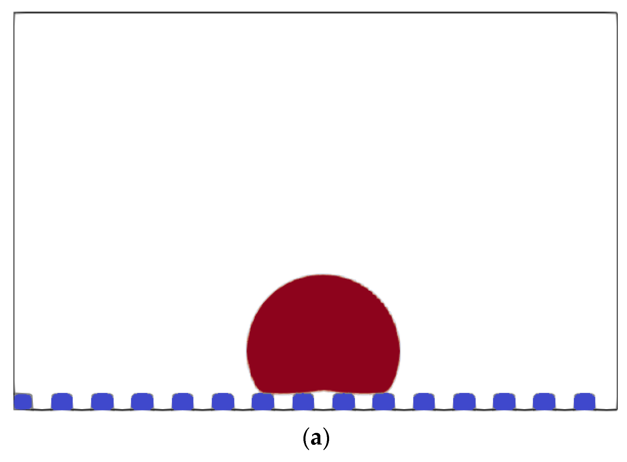
In the present investigation, we varied the Bond number between 0.526 and 1.29 in both Cassie–Baxter and Wenzel states for the static contact angle of 89.3° (expected on a flat surface).
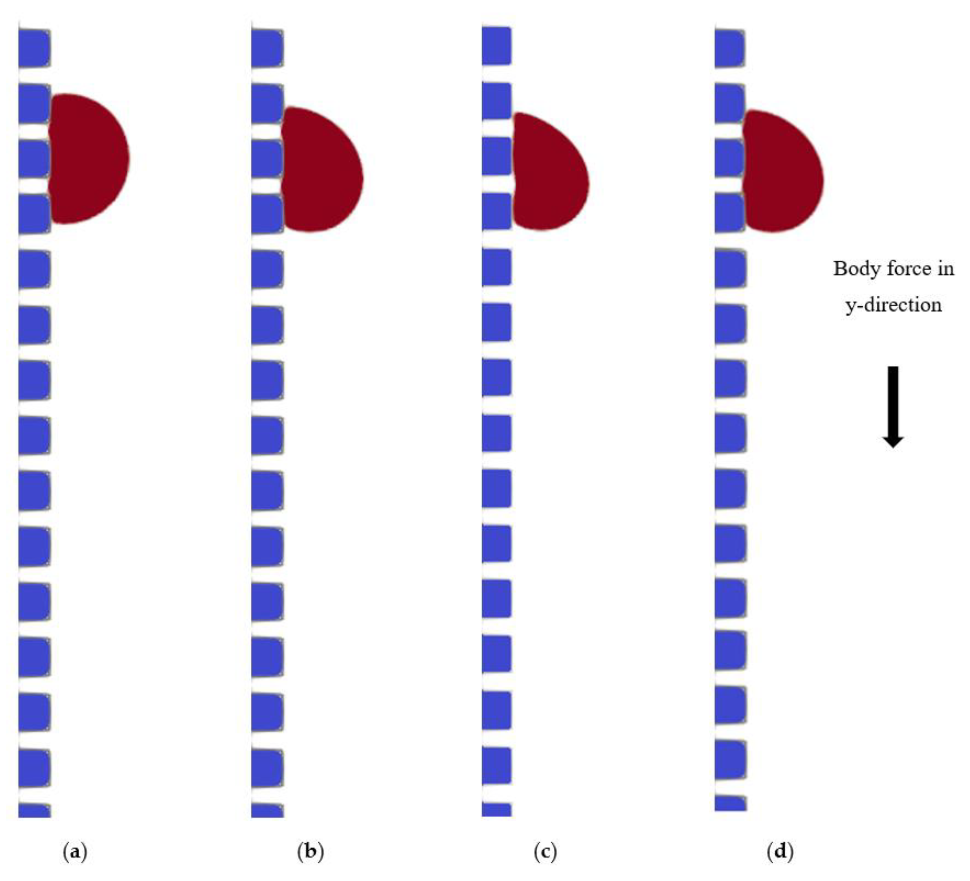
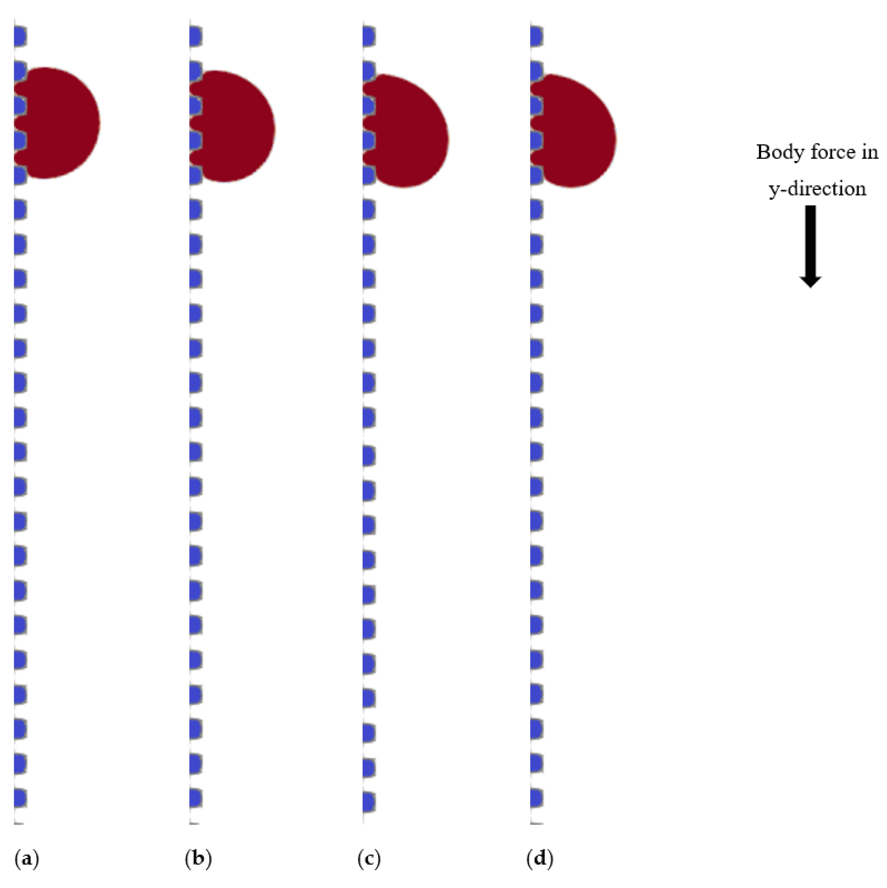
The first case study corresponds to the liquid droplet with a radius of 20 lu under the
g of 2.2 × 10
−6 lu/ts
2 and a Bond number Bo = 0.526. The contact line goes to the next ridge once the receding contact angle achieves its limited value. At the same time, the droplet deforms further until it reaches a balance between capillary and body force (see
Figure 5).
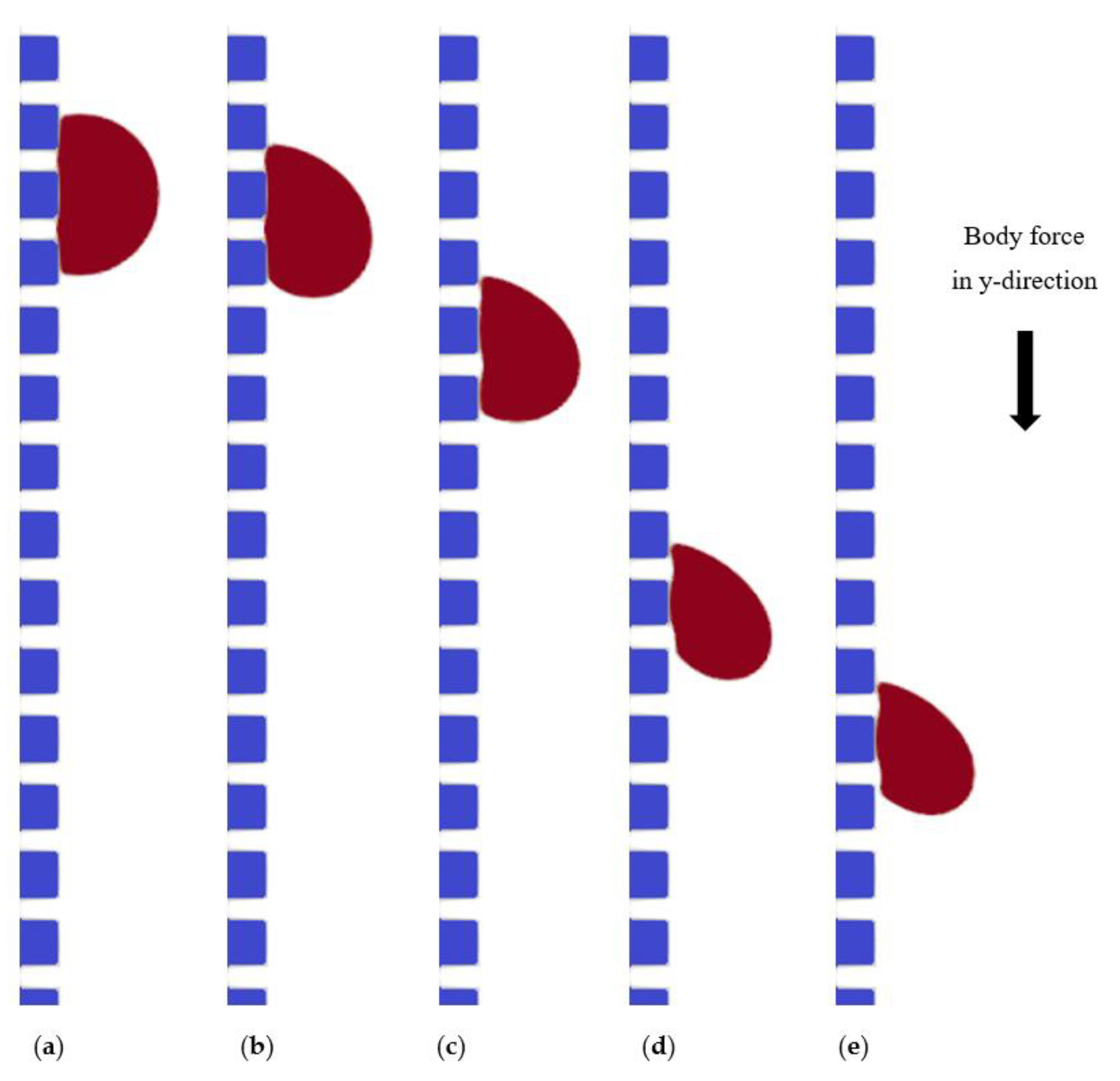
Next, the body force component was varied to adjust the Bond number. At Bond number Bo = 0.704, the movement of the receding contact line from one ridge to another is observed. Once the advancing contact angle reaches the hysteresis window, the droplet motion is prompted. After the droplet motion starts, the receding and advancing contact lines jump from one ridge to the next; in the meantime, the droplet continues to slide over the grooved surface (see
Figure 6).
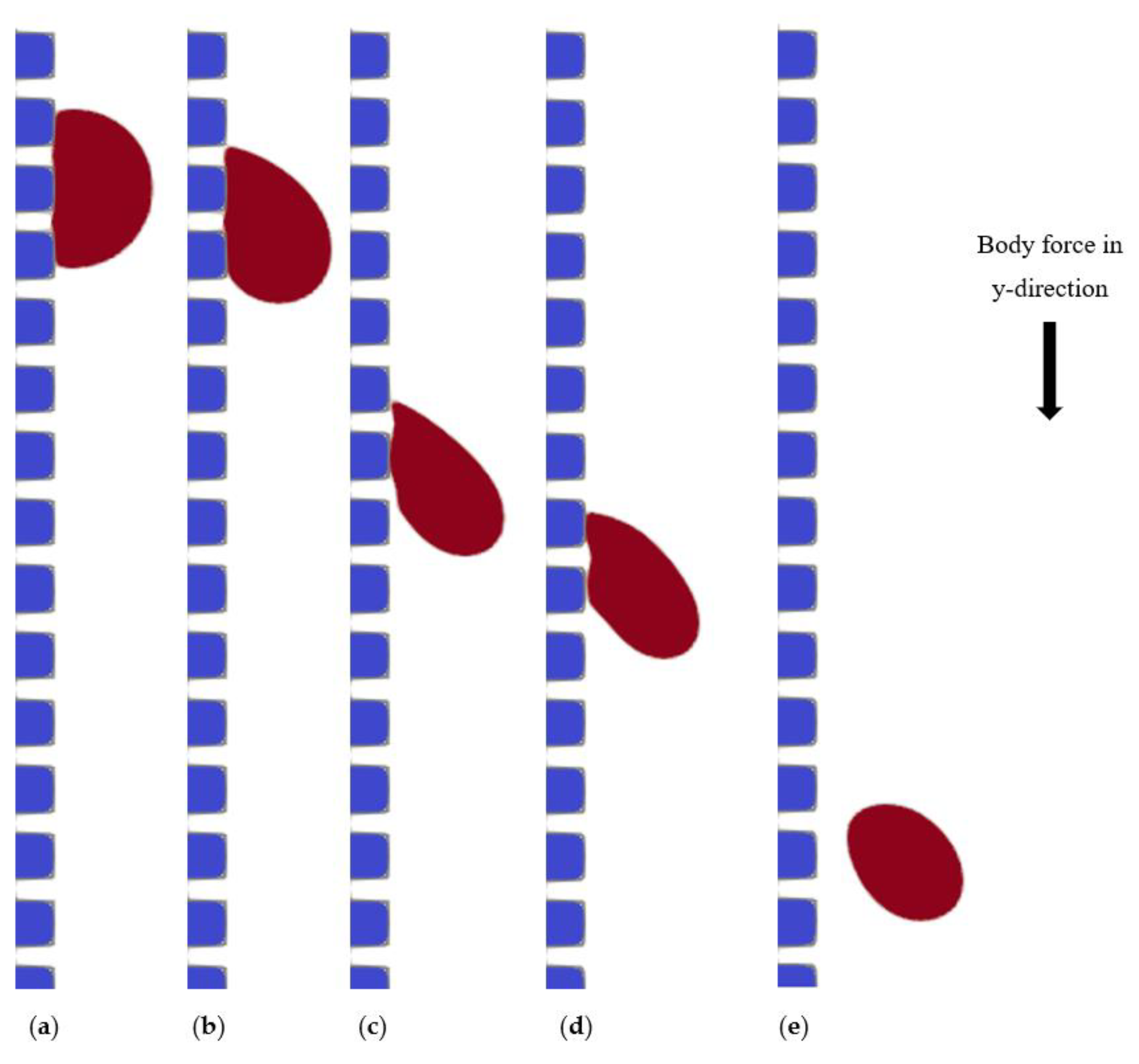
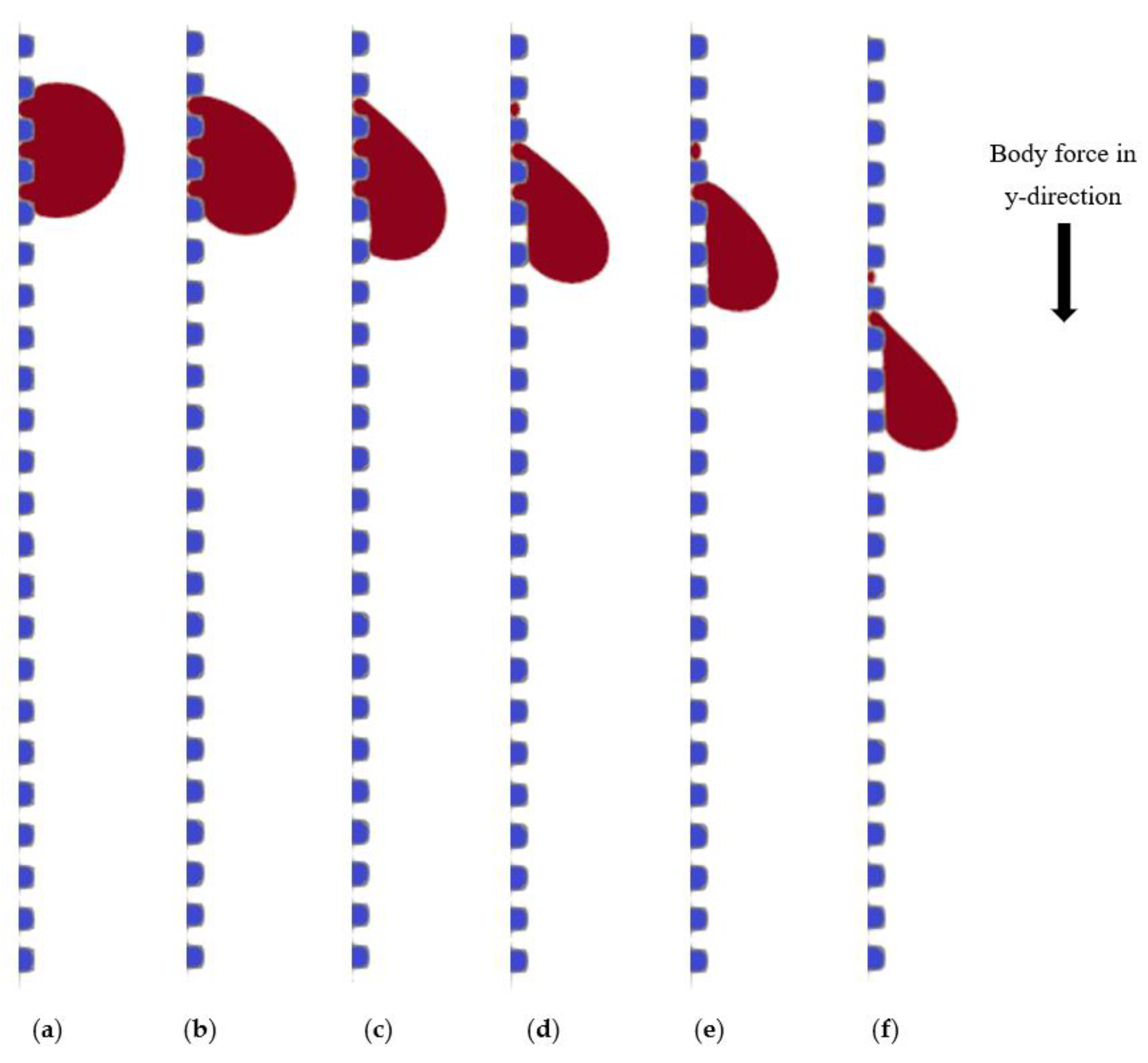
The droplet dynamics dramatically change by increasing the Bond number to 1.29. The droplet contact region with the surface reduces until the droplet fully detaches from the bottom surface. The advancing contact line moves slower than the receding contact line. This state corresponds to a detachment regime (see
Figure 7).
Changing the groove-ridge dimensions to drive the Wenzel state at the Bond number of 0.821 allowed us to determine if any substantial difference was appreciated concerning the Cassie–Baxter state. The Wenzel state increases the wall adhesion to the droplet while only deforming it slightly. The contact line remains static on the substrate (see
Figure 8).
The droplet increases its deformation and starts slipping onto the surface after increasing the Bond number to 0.891. Furthermore, the advancing and receding contact lines move at nearly the same rate, representing a steady state within the fluid system (see
Figure 9).
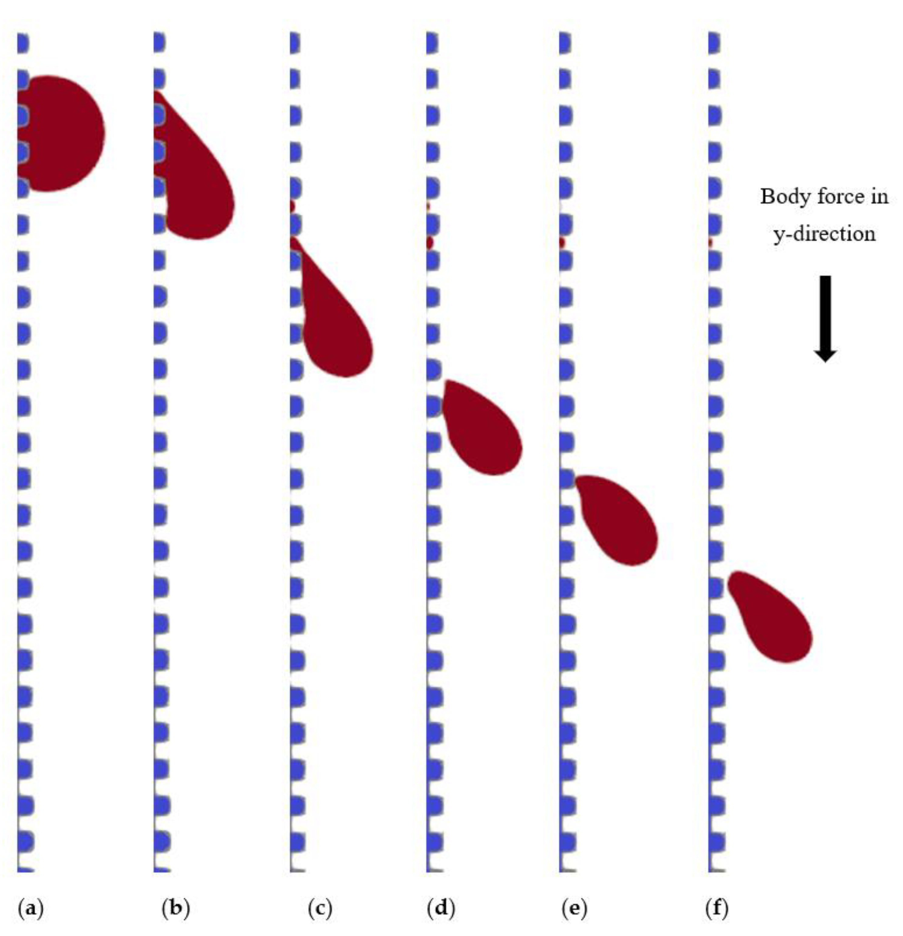
Further increase of the Bond number to 1.05 causes a droplet to stretch until it forms a neck and splits into two separate parts. The surface’s grooves-ridges still trap one part of the droplet, and the remaining part separates from the substrate and descends rapidly (see
Figure 10). Additionally, an entrapment of the fluid in the space between ridges has been observed for slipping and breakup regimes. A similar observation has been noted in studies by Bhardwaj and Dalal [
19].
Therefore, as the Bond number increases, the sliding droplet at Cassie–Baxter and Wenzel states experiences three regimes: stationary, slipping, and detachment. The stationary regime is reached when the contact line remains immobile on the substrate. As expected, the detachment regime occurs at a smaller critical Bond number under the Cassie–Baxter state compared to the Wenzel state.
7. Concluding Remarks
The multiphase SC-LBM model of a 2D weightless sessile droplet spreading on a horizontal grooved surface and its body force-driven slipping on a vertical configuration is presented. Results were obtained for unit density and viscosity ratios between the droplet and the surrounding fluid. Several wettability regimes were explored by varying the groove-ridge dimensions and the static contact angle. The droplet depicted the Wenzel or Cassie–Baxter states in all studied scenarios, even on the vertical wall. The sliding droplet on the vertical wall, driven by a parallel body force, portrayed dynamic contact angles affected by the groove-ridge dimensions and exhibited stationary, slipping, and breakup regimes under both states.
The Bond number was varied from 0.526 to 1.29 and determined the evolution of the sliding droplet, revealing a critical Bond number at which detachment from the wall may occur. As expected for this wetting condition, the critical transitional Bond number was smaller for the Cassie–Baxter state than for the Wenzel state in response to the lower effective contact surface between the droplet and the wall in the former.
Further analysis of the impact of the density ratio, changing it between 0.5 and 4, demonstrated that it does not affect the observed wettability regimes and their critical Bond numbers.
Future work is ongoing to investigate the sliding droplet subject to variations in the geometry and dimensions of various roughness elements. Additionally, the study will be extended to 3D configurations to explore more complex and realistic slipping conditions.


 ,
, 


