1. Introduction
The attitude control system is an important part of spacecraft control system. It affects the flight performance and attitude tracking property, and plays a crucial role in the safe flight mission of spacecraft [
1]. In recent years, many scholars have deeply studied the design of controllers in the case of spacecraft external disturbances, system modeling uncertainties, and actuator faults [
2].
The control methods of spacecraft mainly include adaptive control [
3], sliding mode control [
4], neural network control [
5], model predictive control [
6], fuzzy logic control [
7] and dynamic inversion control [
8], and so on. Sliding mode control is widely used in the field of aircraft control because of its strong robustness to external disturbances and uncertainties of the system. It should be pointed out that most of the current advanced controller designs can prove that the control system is asymptotically stable, that is, the derivative of Lyapunov function
, which theoretically indicates that the system can be stable in an infinite time. In the field of aircraft control, due to the requirements of spacecraft tasks, the system needs to respond quickly; as such, some scholars have proposed the finite time control method. Reference [
9] designed a finite time tracking controller based on fast terminal sliding mode control technology and neural network for a spacecraft attitude control system with sensor failure and actuator saturation. In the stability proof of reference [
9], the Lyapunov function satisfies
, where
, the system will be stable within a finite time
, i.e.,
,
is the initial value of the system state variable. For the rendezvous task of thrust vector spacecraft, a constrained optimal orbit finite time attitude controller design scheme is proposed in [
10]. In reference [
11], a finite time disturbance observer is designed for spacecraft attitude control system with actuator faults and mismatched disturbances, and the estimation is applied to the design scheme of a finite time sliding mode fault-tolerant controller. References [
10,
11] proved that the objective of stability is that the derivative of Lyapunov function satisfies
, where
,
,
, and it can prove that the state of the system converges in a finite time
, and
. It can be seen from [
9,
10,
11] that the proof of finite time convergence of the system is related to the initial value of the system. When the initial value of the system changes or uncertain, it is difficult to calculate the convergence time of the system, which limits the application of finite time control.
In order to solve the problem that the finite time stability is related to the initial value, a fixed time controller with globally fixed convergence time of the system has been proposed. Reference [
12] designed a fixed time attitude controller using fixed time theory and improved inversion control strategy. A fixed time attitude tracking control scheme for rigid spacecraft is proposed in [
13] based on the idea of adding an integrator and inversion control technology. The proof objective of [
12,
13] is to make Lyapunov function satisfy
, where
,
. If the above inequality is satisfied, it can be shown that the system is stable in a fixed time
T, and the expression of
T is
. It can be seen from the proof process of fixed time stability that the fixed time value of system convergence is related to the controller parameters of the system. In most cases, it is difficult to establish a direct relationship between stable fixed time and control parameters. Once the fixed time value of system stability is set, it is difficult to make the system stable through several parameter adjustments. In order to solve the above problems, Sanchez Torres et al. proposed a controller design scheme with a fixed time upper bound as an adjustable parameter, which is named as a predefined-time stable system [
14]. The convergence time of the predefined-time stable system can be preset arbitrarily by designing the parameters of the controller, which is independent of the initial value of the system. At present, the control theory related to the predefined-time stability is mainly applied to fractional order systems [
15], robotic control systems [
16], space robots [
17], surface ships [
18], hypersonic vehicle attitude control systems [
19], etc. To the best of our knowledge, the results about predefined-time fault-tolerant control of spacecraft attitude control systems with external disturbances, system uncertainties and actuator failures are limited, which remains challenging and motivates us to do this study.
Learning observer is an advanced fault diagnosis mechanism, which can estimate constant fault, time-varying fault, and periodic fault. Its basic principle is to use the fault information at the previous time and the state output error information of the system for iterative learning to obtain the estimated value of the fault information at the current time [
20]. For the distributed system, reference [
21] reconstructs the fault value of the system by using the fault information of the previous time and the residual information of the previous time. This kind of observer can be called iterative learning observer. References [
22,
23] use the fault information of the previous time and the estimated error value of the current time state to reconstruct the fault of the system. This kind of observer can be called recursive learning observer. At present, most learning observers are used to estimate additive faults, and there are few research results on multiplicative faults (such as actuator efficiency loss faults).
Based on the above analysis, this paper proposes a predefined-time control scheme based on robust learning observer for a spacecraft attitude control system with external disturbances, system uncertainty and actuator fault. Firstly, the mathematical model of spacecraft attitude control system is given and a learning observer is designed to estimate the efficiency loss fault of the actuator. By using the estimated value of the learning observer, a fault-tolerant controller with predefined-time is designed. Lyapunov function is used to prove that the attitude angle of the system can track the desired command signal within the predefined time. Finally, the numerical simulation proves the effectiveness and feasibility of the proposed control scheme. The contributions of this paper are summarized as follows:
A robust learning observer is proposed to reconstruct efficiency loss faults. Compared with the traditional iterative learning observer [
20] and recursive learning observer [
21,
22], the learning estimation law proposed in this paper is composed of the fault estimation value and state estimation error of the previous time and the state estimation error of the current time, which can quickly and accurately reconstruct the effectiveness value of the actuators.
Using the reconstructed information of actuator efficiency factor, a fault-tolerant attitude controller is designed based on the lemma of predefined-time stability and sliding mode control theory, so that the attitude angle of the system can track the desired command signal within predefined time.
Compared with the finite-time and fixed-time attitude control systems, the convergence time of the predefined-time stable system can be preset arbitrarily by tuning a simple parameter, which is independent of the initial value of the system.
The paper is organized as follows. The spacecraft attitude model and control objective is formulated in
Section 2. The design of learning observer is proposed in
Section 3 while the predefined fault-tolerant controller is given in
Section 4. The simulation results are shown in
Section 5. Conclusions are made in the last section.
2. The Model of Spacecraft and Problem Formulation
In this section, the spacecraft kinematics described using modified Rodrigues parameters and dynamics of attitude loop can be described as
where
denotes the spacecraft attitude angle vector,
denotes the attitude rate vector and is measurable;
denotes the inertia matrix,
denotes the inertia uncertainty;
denotes the control torque vector;
denotes the external disturbance vector;
, and
and
denote cross product matrices which defined as follows
The three-axis attitude control torque of spacecraft is realized by the actuator of the system. This paper considers the situation where the actuators experience a partial loss of actuator effectiveness. Then, the spacecraft attitude dynamics in Equation (
1) can be modified as
where
denotes the control distributed matrix,
denotes the desired control torque allocating to the individual actuator,
m indicates the number of actuators.
denotes the health condition of the actuators, which can be called the actuator effectiveness matrix, and
. When
implies that the
ith actuator is operating healthy without any fault. When
implies completely failure of
ith actuator.
is can be regarded as the lumped disturbance vector.
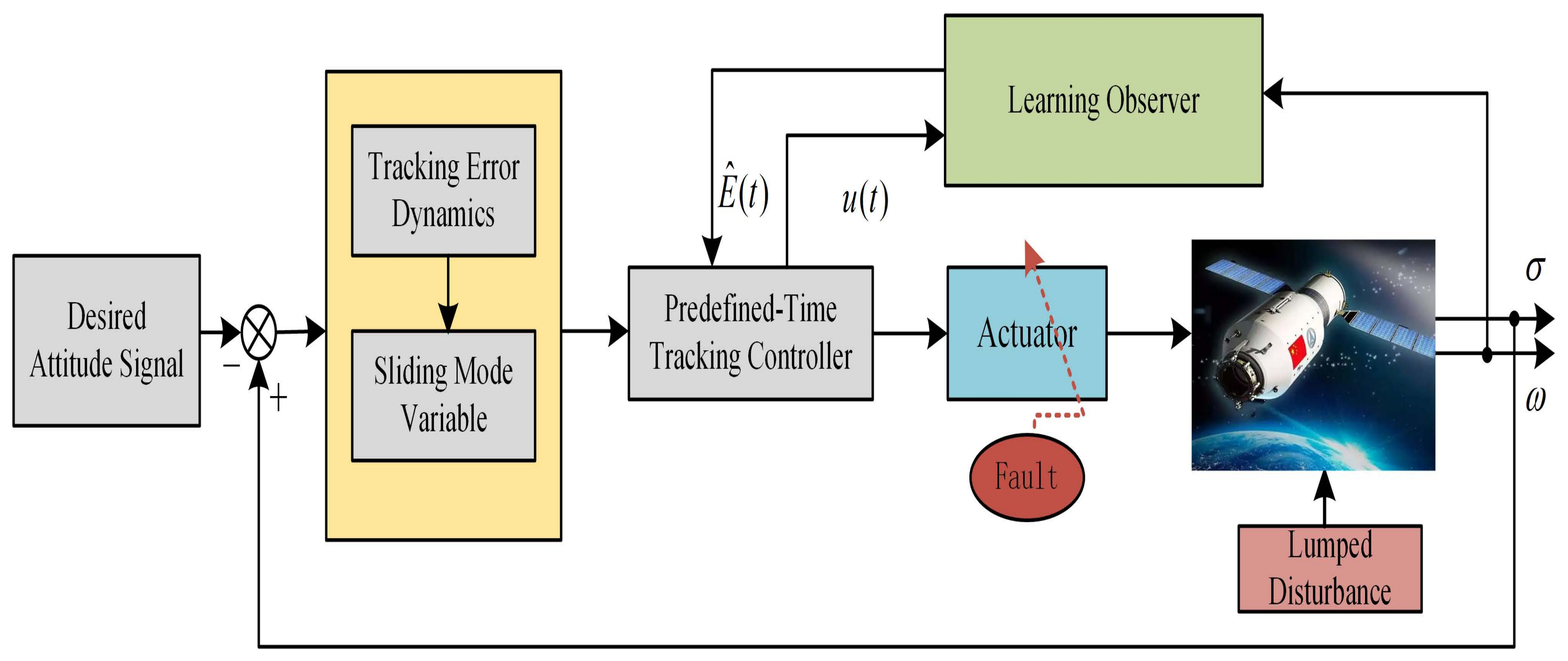
Control objective. For the spacecraft attitude control system with external disturbance, system uncertainty and actuator efficiency loss fault, the efficiency factor in the system is reconstructed by designing a learning observer, and then a predefined-time fault-tolerant tracking controller is designed based on the predefined-time stability lemma and sliding mode theory, so that the attitude of the system can accurately track the command signal within the predefined time. The structure block diagram of the observer-based predefined-time attitude control for spacecraft is designed as shown in
Figure 1.
The following lemma and assumptions are introduced, which will be used for deriving our main results in the sequel.
Lemma 1 (Predefined-time stability [
14])
. For autonomous control systems , if there is exists a Lyapunov function with . Then, it can be concluded that the control system is globally predefined-time stable with respect to T in sense that for all and , provided thatwhere , denotes predefined time value. Assumption 1. The nonlinear function is uniformly bounded for with a Lipschitz constant , which could be formulated in the following Assumption 2. The lumped disturbance vector is bounded, but the upper bound is unknown. Namely, , where is the unknown positive scalar.
Assumption 3. Because of physical limitations on the actuator, the control action generated is limited by the saturation value, and for simplicity, we assume that all the actuator control input torques have the same constraint value , that is, for .
3. Design of Learning Observer
Inspired by the previous learning observer design [
24], we designed an improved learning observer design scheme for the efficiency factor of the actuator. The actuator loss of effectiveness fault
is a diagonal matrix, and
in Equation (
2) can be written as
where
and
.
The faulty dynamics equation of rigid spacecraft (2) can be transformed into
An improved learning observer is designed as follows
where
and
denote the angular velocity estimation and loss effectiveness fault estimation, respectively.
denotes the last time value and
is usually taken as the sampling time internal of the system. Signal
is also called learning observer input, which is updated or driven successively by the state estimation error at the past and current time, and previous learning observer input
.
l is a positive constant and
and
are positive-definite gain matrices chosen by designer.
n is a positive sign function gain. The parameter
is a positive-definite matrix.
Remark 1. In order to ensure that our estimated fault value remains within an interval , we improve our learning update law (6) as followswhere indicates the lower limit of the efficiency loss factor, which is usually set to a very small value, such as . stand for projection operator. To evaluate the estimation performance of the robust learning observer, two new variables have been defined as follows
and
. The observer error equation can be obtained by subtracting (7) from (6)
In order to express the main results, the following assumptions and lemmas are required.
Assumption 4. Since the efficiency loss factor of the actuator satisfies the constraint , the following inequality can be held as , where is a positive constant.
Lemma 2. If learning update law is defined in Equation (6), the following inequality holds:where and is a number greater than 0, and its value will be given in the proof section. Proof. The efficiency factor estimation error of the observer is
Using the well-known Young’s inequality, that is
for all
, we have, for arbitrary positive constants
,
Combining above inequalities into (11) leads to
where
,
,
and
. This completes the proof. □
Theorem 1 (Main Result)
. Consider estimation error Equation (9) satisfying Lemma 1. An improved learning observer is designed in the form of (7) with the observer gains selected as , , and , then efficiency factor estimation error and the state estimation error will converge to a small interval containing the origin. Proof. Select the Lyapunov function as follows
Taking the time derivation of
yield
Substituting (9) into
, (16) can be further obtained as follows
Using the Young inequality principle, the following inequality holds
where
is a positive constant. Substituting the inequality (18) into (17) leads to
where
is a positive constant.
Substituting Lemma 2 and Assumption 4 into Equation (
18), one has
Then, if the gain of the learning observer satisfies the following inequalities,
the derivation of
respect to time yields to
where
. It is further obtained from inequality (21) that
when
or
. According to theorem in [
25], it can be concluded that the learning observer error system is uniformly ultimately bounded.
Correspondingly, it is concluded that the estimation errors of angular velocity and fault are ultimately uniformly bounded by
By adjusting the parameters to increase the value of and or decrease the value of , the estimation error of the observer can converge to arbitrarily small residual interval. Then, the proof of Theorem 1 is completed. □
4. Design of Predefined-Time Attitude Tracking Controller
In this section, a predefined-time attitude fault-tolerant tracking controller is designed by using the lemma of predefined-time stable and the reconstructed information
, which can be obtained by learning observer, where
.
is defined as the estimation error matrix, which satisfies
. From Theorem 1,
converges to an arbitrarily small value, and hence the following inequality can be achieved
, where
is a unknown positive constant. The mathematical model expression of spacecraft attitude control system can be rewritten as
For the faulty attitude system (23), define two new error variables
,
, where
is the desired attitude command; therefore, the attitude tracking error dynamics can be expressed as
Define the Lyapunov function of attitude angle error
. Select a sliding mode variable as follows
where
,
, and
is the predefined time value.
According to Lemma 1, the predefined-time attitude tracking controller can be expressed as
where
,
is the predefined time value.
is the estimation of efficiency factor, which can be obtained from learning observer (7).
denotes the pseudo-inverse operation of the matrix
.
is the parameter gain of the system and its value is taken as
.
is the Lyapunov function of sliding mode variable,
.
Theorem 2. For the faulty spacecraft attitude systems (23), by designing a fault-tolerant controller based on the estimation information from the learning observer (7), the control system can be stabilized in the predefined time , and the attitude of the system can track the desired attitude angle command in the predefined time T.
Proof. Derivation of the Lyapunov functions
on sliding surfaces variable, we can obtain
Substituting control law (26) into above equation gives
According to Lemma 1, when , and sliding mode variable s will converge to 0 in the predefined time .
When
, combining with (25), we have
Taking the derivative of
with regard to time
t, one has
According to Lemma 1, when , tracking error vector will converge to 0 within the predefined time . In conclusion, the attitude system of the spacecraft will be stable within the predefined time under the action of the controller, and the attitude angle of the system will track the reference command within the predefined time T. The proof of Theorem 2 is completed. □
5. Simulation
In order to verify the effectiveness and feasibility of the control scheme proposed in this paper, a learning observer (LO) and a predefined-time controller (PTC) are designed for a class of spacecraft operating in circular orbit. At the same time, they are compared with the existing adaptive sliding mode observer (ASMO) [
26] and terminal sliding mode control (TSMC) schemes [
10].
The initial value of attitude angle and angular rate of spacecraft attitude control system is set as
and
. The learning time interval of the learning observer is
. The external disturbance is set to
. The moment of inertia of the system is set to
. In this section, we consider that the number of actuators is
, and they are installed orthogonally, that is,
D is the identity matrix. The desired attitude angle command is
. The design controller parameters and the observer values are given in
Table 1.
In the simulation, the following two cases are considered.
Case 1. Proposed LO vs. adaptive sliding mode observer in [
26].
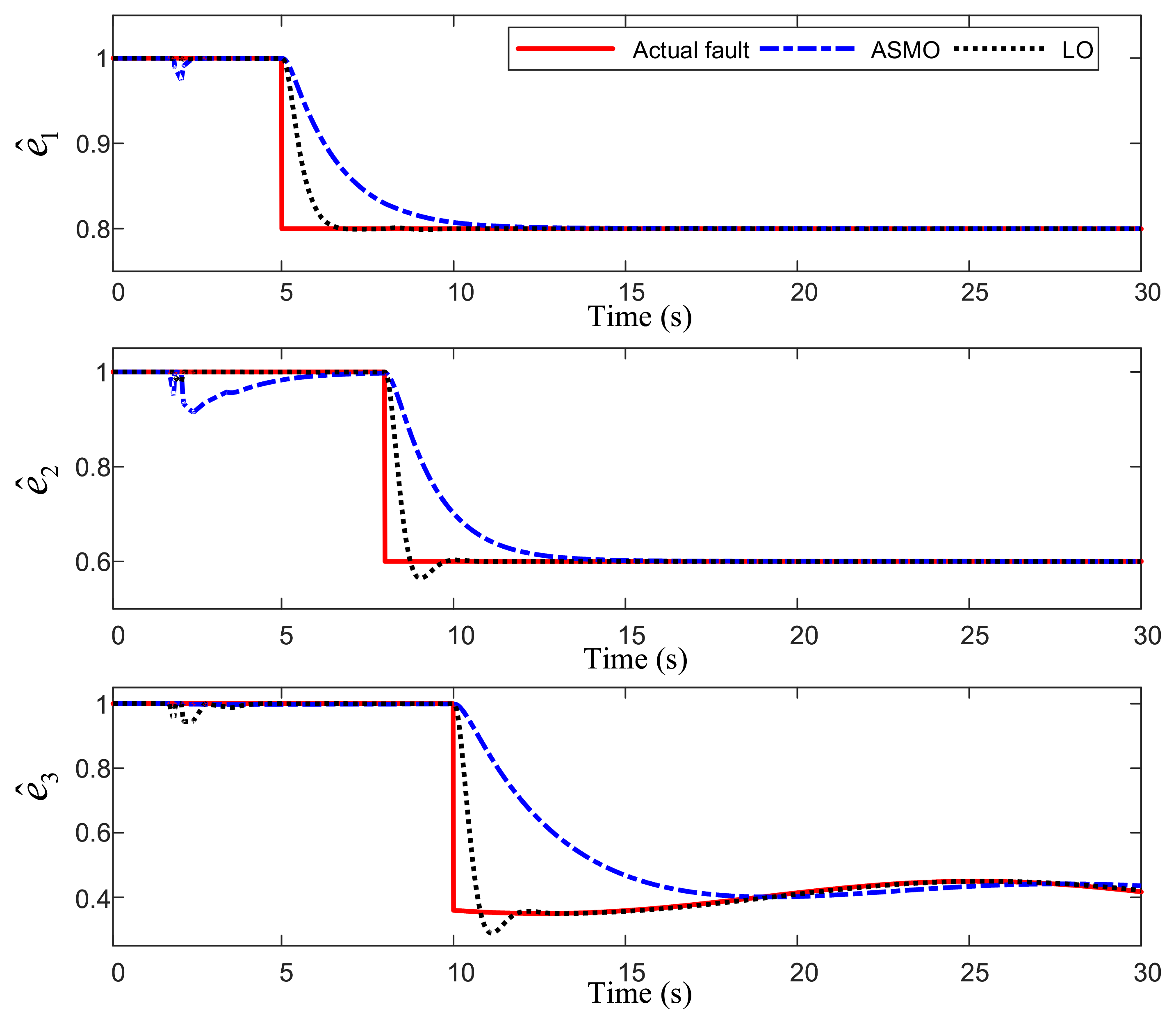
In this case, the main purpose is demonstrating the validity of the proposed learning observer approach. In order to facilitate the analysis, We set different efficiency factors on the three actuators: constant or time-varying faults. Denote
and the fault scenario is set as
Figure 2 shows the response curve of fault reconstruction by two observers. The two observers have good estimation performance for constant faults, but the adaptive sliding mode observer can not estimate time-varying faults well.
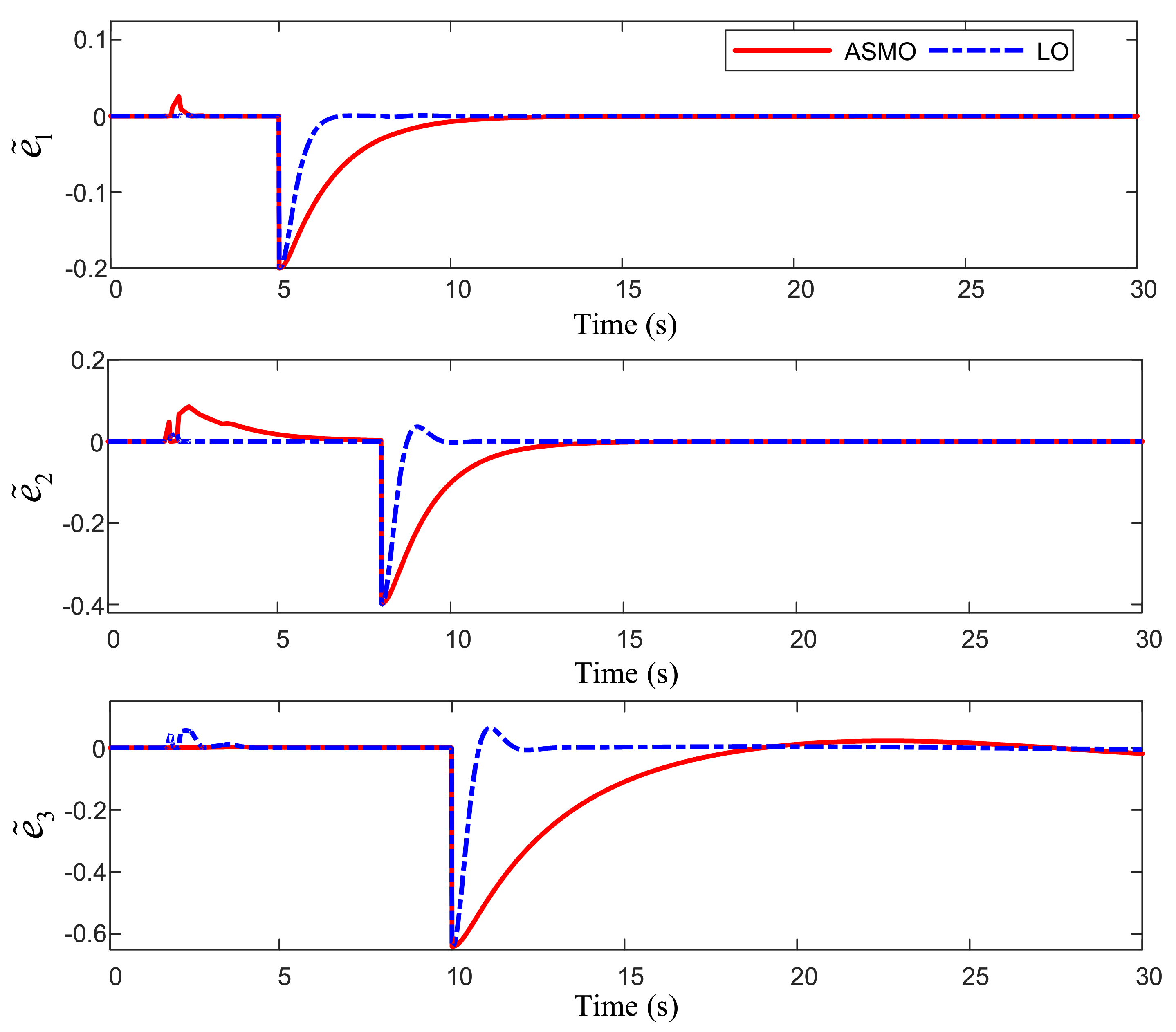
Figure 3 shows the fault estimation error curves of the two observers. When no efficiency loss fault occurs in the system, the adaptive sliding mode observer is greatly affected by the comprehensive disturbance. The estimation error of the second channel
fluctuates greatly. It takes 5 s for the adaptive sliding mode observer to make the estimation error converge to a small range. When the efficiency loss fault occurs, the learning observer can accurately estimate the efficiency factor in about 3 s. It can be seen from the
Figure 4 that no matter what form of efficiency loss fault occurs, the learning observer can accurately reconstruct the fault factor within 3 s after the fault occurs. Compared with the learning observer, the adaptive sliding mode observer takes a longer time (about 8 s) to track the constant fault; however, for the time-varying fault, their estimation results are poor and there is a large estimation error.
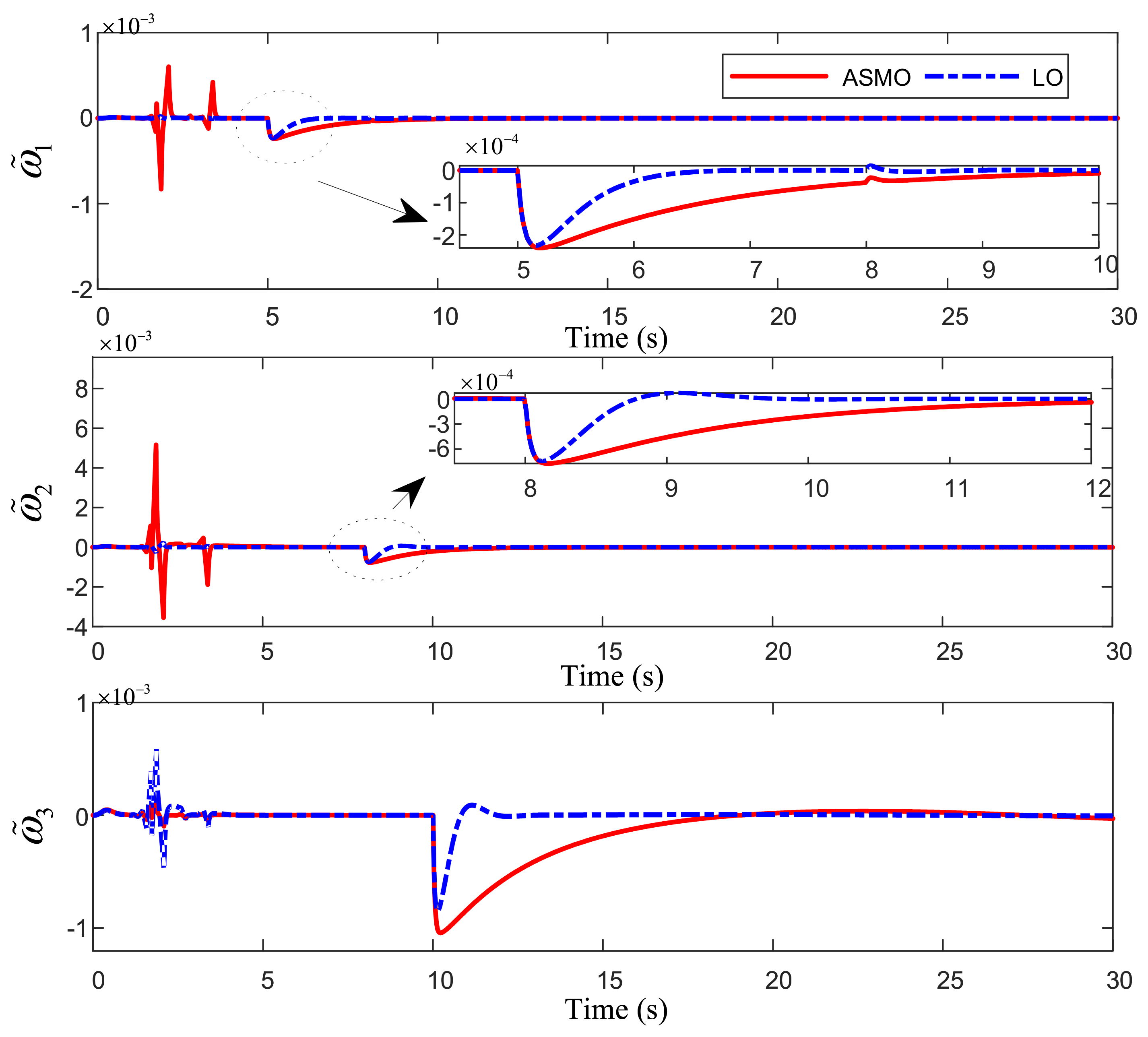
Figure 4 shows the estimation error curve of system state variables
. Both observers have good estimation effect on the state variables of the system, and the estimation error converges to a very small interval. In conclusion, the learning observer proposed in this paper can quickly and accurately estimate the efficiency loss failure (constant or time-varying) of the actuator.
Case 2. Proposed LO-based predefined-time controller (PTC) vs. terminal sliding mode controller (TSMC) in [
10].
For comparison, a terminal sliding mode fault tolerant controller is implemented in the attitude control system.
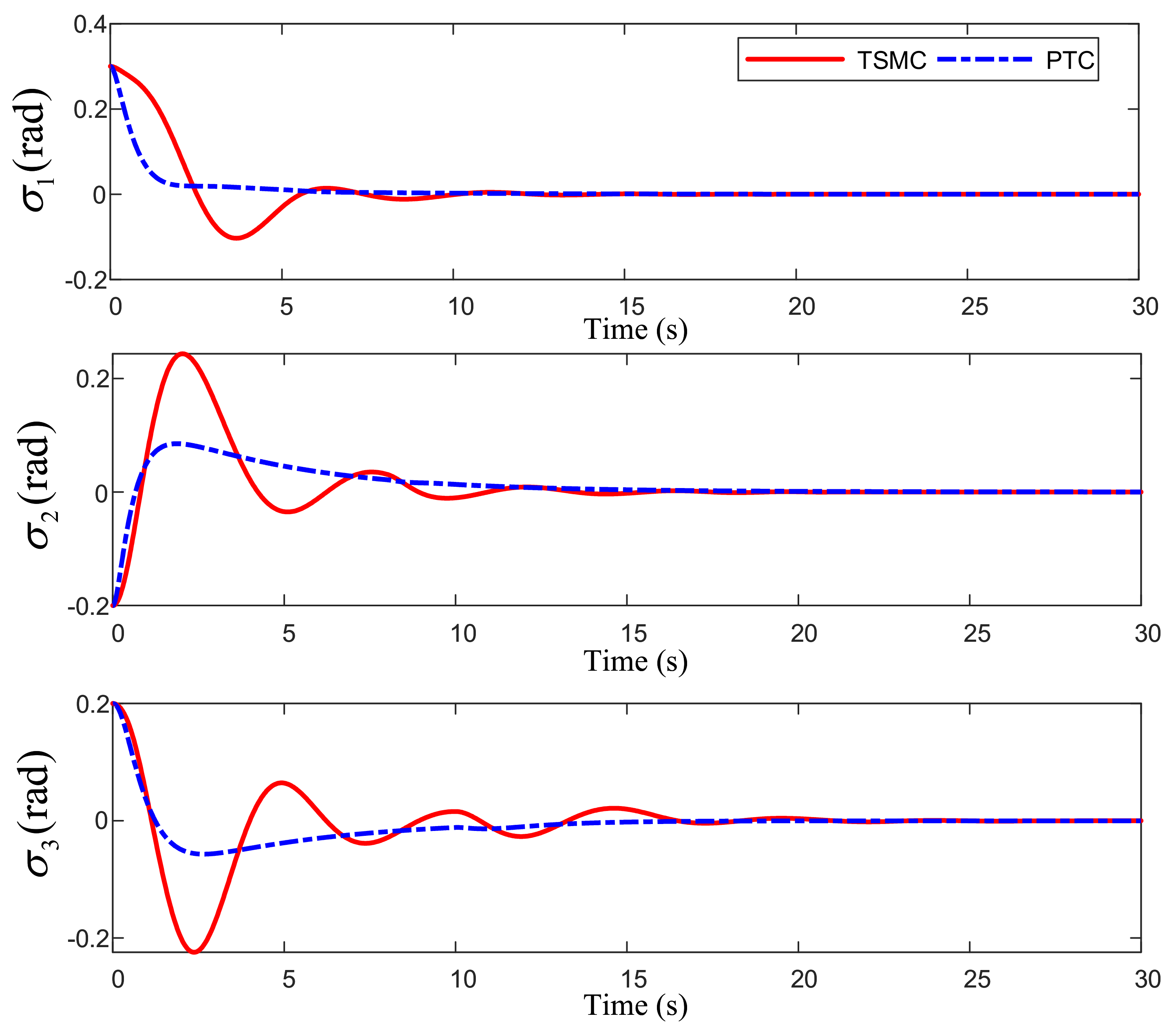
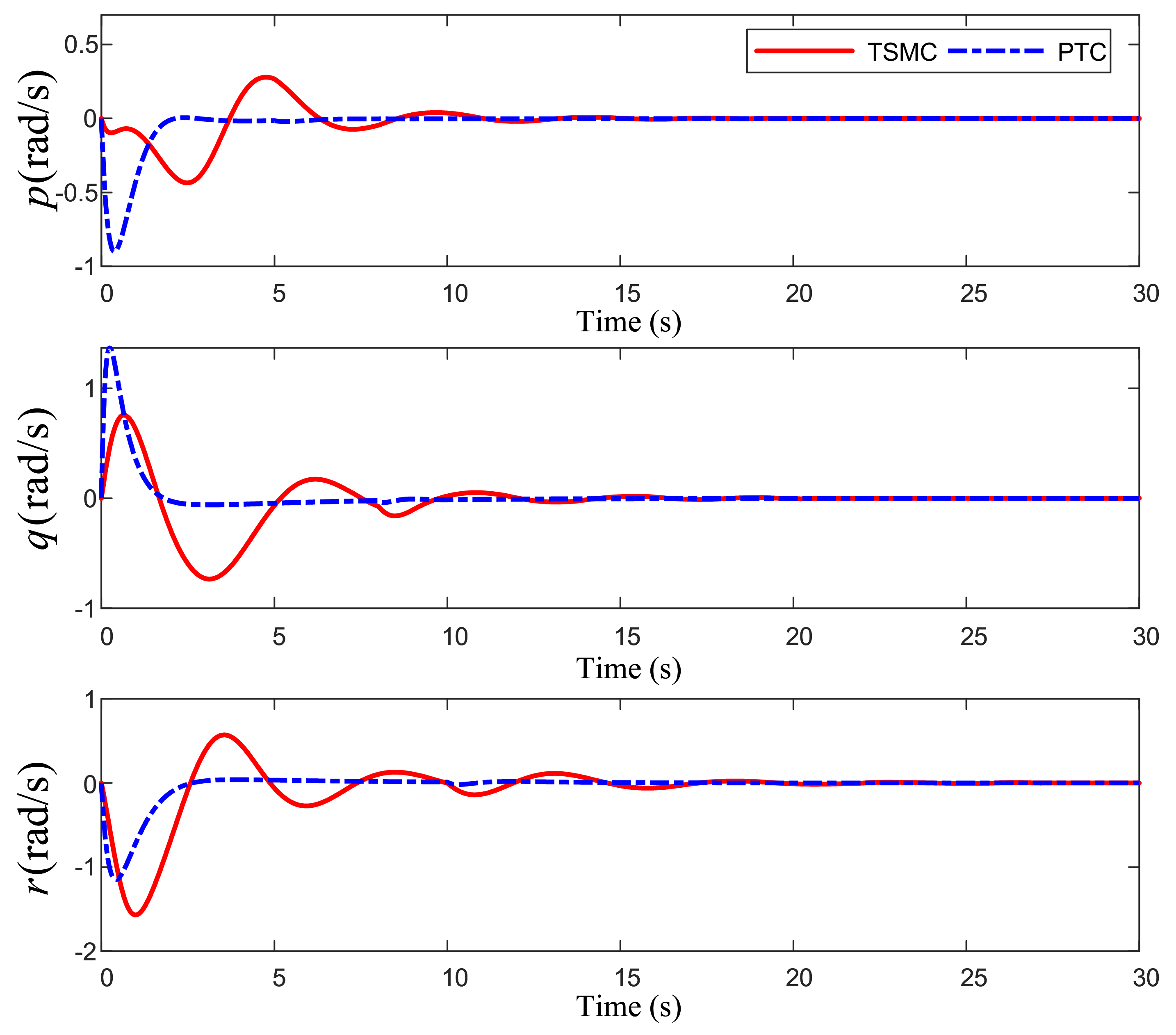
Figure 5 demonstrates the attitude angle tracking performance and
Figure 6 shows the response of system angular velocity.
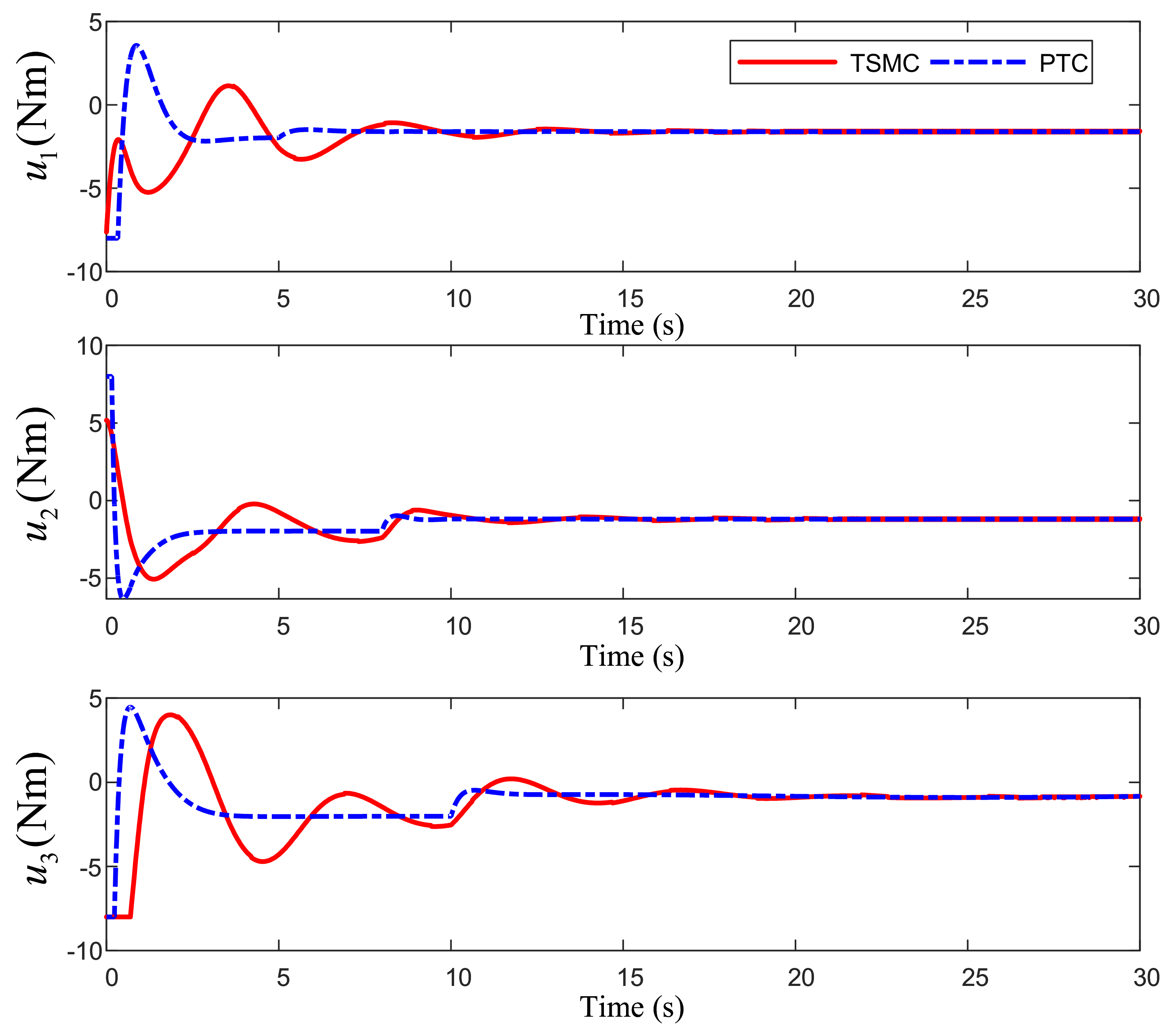
Figure 7 is the response of actuator torque under the two different control methods. It can be seen from
Figure 5 that the system attitude angle changes gently under the predefined-time controller, and the attitude angle tracks the reference command within 20 s.
Figure 6 and
Figure 7 show that the output torque of the actuator directly affects the angular rate change of the system. When each actuator appears, the control torque change of the scheme proposed in this paper is relatively gentle, which will not cause a large range of changes in the angular rate curve. When no fault occurs (the first 5 s), the angular rate converges to the neighborhood of 0 in 3 s. At the time of failure, the attitude angular rate has only a small fluctuation, and then returns to the stable state within 2 s.
Overall, the results of the above two cases fully verify the stability and robustness of the learning observer-based predefined-time tracking control system under external disturbances, system uncertainties and loss of actuator effectiveness.


