Article

Static Voltage Stability Assessment Using a Random UnderSampling Bagging BP Method

1
School of Electrical Engineering, Beijing Jiaotong University, Beijing 100044, China
2
College of Energy and Electrical Engineering, Hohai University, Nanjing 211100, China
*
Author to whom correspondence should be addressed.
Processes 2022, 10(10), 1938; https://doi.org/10.3390/pr10101938
Submission received: 22 August 2022 / Revised: 17 September 2022 / Accepted: 19 September 2022 / Published: 26 September 2022
(This article belongs to the Special Issue Modeling, Analysis and Control Processes of New Energy Power Systems)

Abstract

:
The increase in demand and generator reaching reactive power limits may operate the power system in stressed conditions leading to voltage instability. Thus, the voltage stability assessment is essential for estimating the loadability margin of the power system. The grid operators urgently need a voltage stability assessment (VSA) method with high accuracy, fast response speed, and good scalability. The static VSA problem is defined as a regression problem. Moreover, an artificial neural network is constructed for online assessment of the regression problem. Firstly, the training sample set is obtained through scene simulation, power flow calculation, and local voltage stability index calculation; then, the class imbalance problem of the training samples is solved by the random under-sampling bagging (RUSBagging) method. Then, the mapping relationship between each feature and voltage stability is obtained by an artificial neural network. Finally, taking the modified IEEE39 node system as an example, by setting up four groups of methods for comparison, it is verified that the proposed method has a relatively ideal modeling speed and high accuracy, and can meet the requirements of power system voltage stability assessment.

1. Introduction

Voltage stability [1] is the main limiting factor for the safe and reliable operation of power systems. With continued load growth and the penetration of new energy sources, modern power systems have been pushed to operate closer to their voltage stability limits. Over the past few decades, great efforts have been devoted to investigating the mechanisms of voltage instability and developing effective voltage stability assessment (VSA) methods [2].
Generally, voltage profiles show no anomalies before undergoing a voltage collapse due to load changes. Voltage stability margin (VSM) is a static voltage stability index that quantifies how “close” a particular operating point is to the point of voltage collapse [3]. Therefore, the VSM can be used to estimate the steady-state voltage stability limit of a power system. Knowing voltage stability margins is critical for utilities to operate their systems safely and with reliability. The system operator must provide an accurate and fast method to predict the voltage stability margin to initiate the necessary control actions [4].
That proposed a static voltage stability prediction method based on gradient boosting, which has better prediction accuracy [5]. However, its training set data are obtained through the calculation of the cumulative probability function (CPF), which is only applicable to a fixed load power factor case. Ghiocel et al. [6] proposed a new method to directly eliminate the singularity by reformulating the power flow problem. The central idea is to introduce an AQ bus in which the bus angle and the reactive power consumption of a load bus are specified. However, the computation burden is still heavy, and the solution speed cannot meet the requirement of real-time assessment.
With the boom of wide-area measurement systems in smart grids [7,8,9], the availability of large amounts of data acquired by phasor measurement units (PMUs) presents a huge opportunity for data-driven stability assessments. Great efforts have been made to perform such tasks through machine learning techniques.
In [10], a static stability assessment method for a power system based on a decision tree algorithm is proposed, which improves the assessment speed. However, there is no countermeasure for the decision tree over-fitting problem. Lai et al. [11] proposed a transient voltage stability assessment model based on convolutional neural networks, which improves the assessment speed by using statistical analysis for data dimensionality reduction. However, relying only on statistical analysis for data dimensionality reduction, it is easy to ignore individual features. Liang et al. proposed a random forest model for static voltage stability assessment, which makes up for the assessment defects of a single decision tree [12]. However, the selection of features is based on subjective judgment. The voltage stability assessment problem is treated as a classification problem of machine learning, making it difficult to accurately know the degree of voltage stability.
A common feature of these machine learning-based efforts is that they assume that the learning dataset can be generated by system simulations in the desired quantity [13]. Since accurate simulation and modeling, especially load modeling, are considered a great challenge in power systems, errors are inevitably introduced into the learning dataset. Preferably, the learning dataset can be obtained from PMU records, which will significantly improve the quality and reliability of the knowledge base. However, learning machines are likely to suffer from severe class imbalance problems. The system remains stable after most disturbances and becomes unstable only in a few cases. If not handled properly, this imbalance can greatly deteriorate the performance of the learning machine, and the minority class will be ignored and thus leading to misjudging. The class imbalance problem exists not only in the field of power systems, but also widely in other academic and industrial contexts, such as credit fraud detection, biomedical diagnosis, equipment fault diagnosis, and Internet intrusion [14].
Faced with class imbalance problems [15], considerable efforts have been made by machine learning researchers to deal with them [16,17]. Synthetic sampling is the most commonly used method for rebalancing class distributions. However, it cannot be directly applied to voltage stability assessment. Because datasets created by naive replication or linear interpolation may not exist in practice. Besides sampling-related techniques, some cost-sensitive tricks are proposed to build cost-sensitive classifiers. By attaching costs to different classes, these techniques manage to enhance minority learning by drawing more attention to minority classes [18].
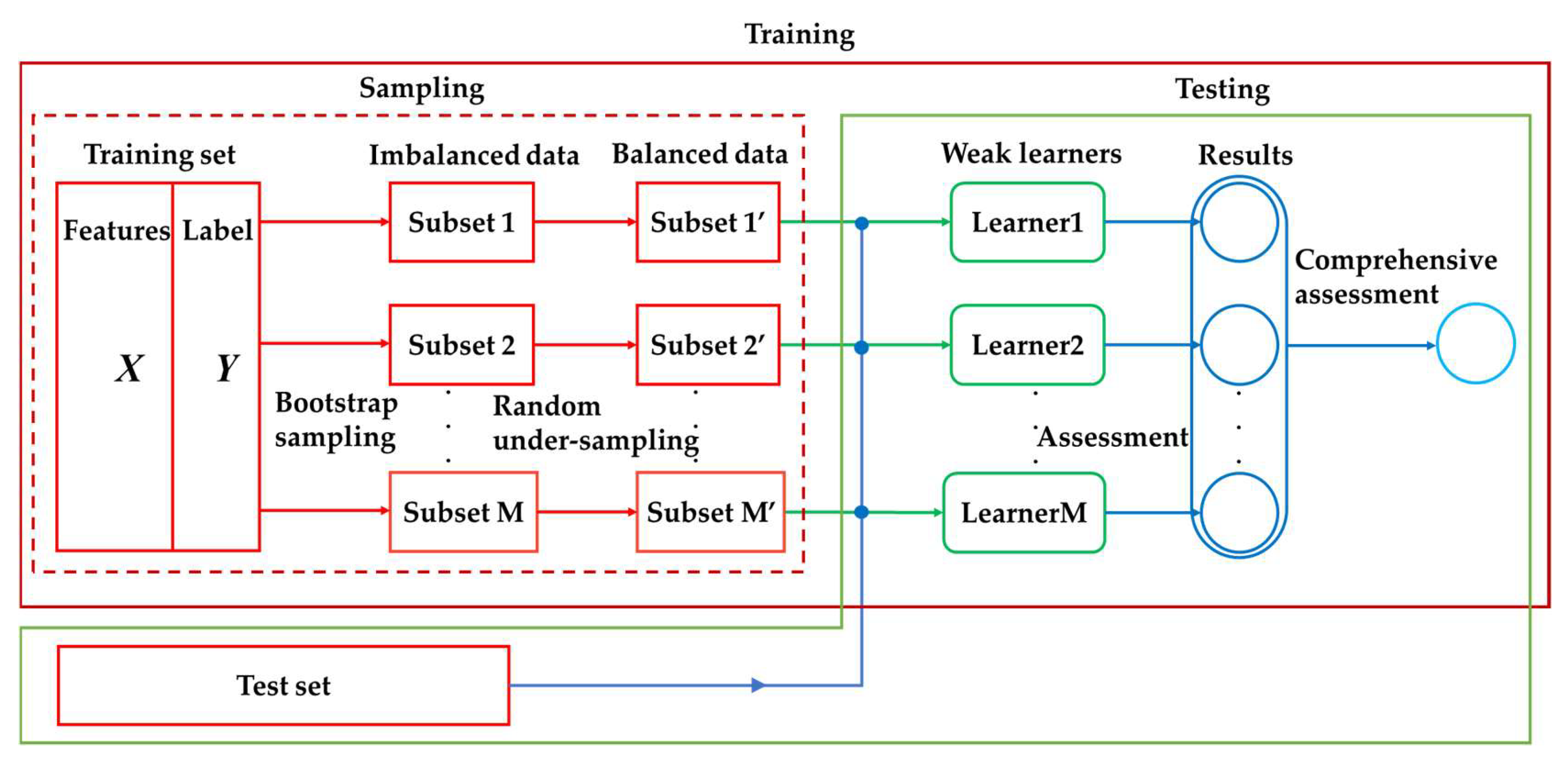
To meet the requirements of voltage stability assessment and solve the problem of class imbalance and poor model generalization in machine learning, an online assessment method of static voltage stability using the RUSBagging method is proposed. The method differs from other methods in that:
The problem of VSA is defined as a machine learning regression problem, which is helpful for grid operators to observe the voltage stability state of the power system.
The bagging method of the ensemble framework is used to build the model to improve the generalization ability of the model.
The random under-sampling method is added to bagging, which solves the class imbalance problem to a certain extent and improves the assessment accuracy on minority class samples.

2. Local Voltage Stability Index

Commonly used static voltage stability indexes are [19,20]: the Jacobi singular value index, voltage sensitivity index, load margin index, VCPI index, and local voltage stability index. Compared to other voltage stability indices, the local voltage stability index (L index), which can give normalized index values for different systems, and which is not limited by the randomness of the direction of load growth, are highly applicable and highly accurate.
By the KCL law (Kirchhoff’s current law) there is Y V = I , where Y stands for node admittance, V stands for node voltage, and I stands for node current. In addition, according to the value of the node injection current, the network nodes are divided into generator nodes, load nodes, and contact nodes, and the equations of the node network after the division are as follows.
[ I G I L 0 ] = [ Y G G Y G L Y G K Y L G Y L L Y L K Y K G Y K L Y K K ] [ V G V L V K ]
where V G and I G are the voltage and current vectors at the generator node, V L and I L are the voltage and current vectors at the load node, and V K is the voltage vector at the contact node.
By eliminating the contact nodes, the remaining nodes in the network are divided into the set of generator nodes ( α G ) and the set of load nodes ( α L ), and Equation (1) can be transformed as:
[ I G I L ] = [ Y G G Y G L Y L G Y L L ] [ V G V L ]
where Y G G = Y G G Y G K Y K K 1 Y K G , Y G L = Y G L Y G K Y K K 1 Y K L , Y L G = Y L G Y L K Y K K 1 Y K G , Y L L = Y L L Y L K Y K K 1 Y K L .
Substituting Z L L = Y L L 1 into Equation (2) converts to:
[ I G V L ] = [ Y G G Y G L Z L L Y L G Y G L Z L L Z L L Y L G Z L L ] [ V G I L ]
Reference [15] gives the local voltage stability index L j for load node j:
L j = | i α L | Z j i * S ˜ i Z j j * V ˙ i | V ˙ j | V j 2 Y j j = | i α L Z j i * S ˜ i V ˙ i | V j
where V ˙ i , V ˙ j are the voltage phases of nodes i, j respectively. S ˜ i is the equivalent load of node i. Z j i * is the mutual impedance conjugate between loads j,i of the equivalent load impedance matrix Z L L . Y j j is the self-conductance of the jth node of the equivalent load conductance matrix Y L L .
The local voltage stability index for all load nodes in the network forms the overall system stability index vector L = [ L 1 , L 2 , L n ] , n α L and the maximum index value for the load is selected to define the voltage stability index for the system.
L = L
The relationship between local voltage stability index and system voltage stability is [21]:
L < 1, system voltage stability.
L = 1, system voltage critical stability.
L > 1, system voltage instability.

3. Random Under-Sampling Bagging BP Method for VSA

3.1. BP Neural Network for Regression of VSA

Since the VSA problem is defined as a machine learning regression problem in this article, a model is built to implement the regression. The back-propagation (BP) neural network model is easy to build, has a wide range of adaptability, and the algorithm is easy to implement. Hence, BP neural network is selected to solve this regression problem.

3.1.1. Model of BP Neural Network for Regression of VSA

Neural networks have an adaptive character, changing the weight values during the training process to suit different requirements [22,23]. The internal neural network can be divided into input, hidden and output layers according to the different functional layers.
For regression of the VSA problem, the input variables are the operating states of the power system, such as nodal voltage, branch power flow, and load demand. The output of the model is the L index, which is the result of the voltage stability assessment.
Where X is the input column vector; x i is the element in row i. W is the weight matrix; specifically, an element of W can be represented by w f , i j . The subscript f indicates the corresponding layer, and the subscript ij indicates the connection between node i in this layer and node j in the next layer. Y is the output column vector; y i is the element in row i. Σ is the summation symbol, which sums multiple input signals; φ i is the activation function of the i-th neuron in the hidden layer and ϕ i is the i-th neuron activation function in the output layer; θ i is the i-th neuron threshold in the hidden layer and b i is the i-th neuron threshold in the output layer.
Neural networks use a large number of hidden layer neurons for data flow processing and network training. Without loss of generality, the neural network data stream processing process is briefly described using a single neuron in Figure 1 as an example.
Assuming that the output of the i-th neuron in the hidden layer is, the output of the ith neuron can be represented by Equation (6) from Figure 1.
o i = φ i ( j = 1 n w 1 , i j x j + θ i )
Similarly, it can be deduced that the output of the ith neuron in the output layer is:
y i = ϕ i ( j = 1 m w 2 , i j o j + b i )

3.1.2. Algorithm of BP Neural Network for Regression of VSA

The learning process consists of two processes: forward propagation of the signal and backward propagation of the error. The forward propagation process is shown in Equations (6) and (7). If the actual output of the output layer is not equal to the label value, then it is transferred to the error backpropagation process. The core of the BP neural network is the error back propagation process.
The error back propagation is to backpropagate the output error in a certain form through the hidden layer, and the error is apportioned to all neurons in each layer according to certain rules. To obtain the error signal of the neurons in each layer, and use it as the basis for correcting the weights of each neuron, the specific correction method is shown in Equations (8) to (11). The process of weight correction is also the learning process of the network. In general, this process continues until the network output error is within the set range or until a predetermined learning time or iterations.
Δ w 2 , i j = η p = 1 P k = 1 K ( T k p o k p ) ϕ i o j
Δ b i = η p = 1 P k = 1 K ( T k p o k p ) ϕ i
Δ w 1 , i j = η p = 1 P k = 1 K ( T k p o k p ) φ i w 2 , i j ϕ j x j
Δ θ i = η p = 1 P k = 1 K ( T k p o k p ) φ i w 2 , i j ϕ j
where Δ w 2 , i j is the weight correction between the i-th neuron in the hidden layer to the j-th neuron in the output layer. Δ b i is the threshold correction for the i-th neuron in the output layer. Δ w 1 , i j is the weight correction between the i-th neuron in the input layer to the j-th neuron in the hidden layer. Δ θ i is the threshold correction for the i-th neuron in the hidden layer. p is the sample index and P is the total number of training samples. η is the weight correction learning rate. T k p is the expected output value of the kth output neuron for the pth sample data.

3.2. Random Under-Sampling Bagging for Improving Model Accuracy of VSA

In the actual operation of the power system, the system is in a stable state in most cases. Stable data is far more than unstable data or critically stable data, which is a typical data imbalance problem. In fact, for the stable operation of the power system, the value of unstable or critically stable sample data is higher than that of stable sample data. Therefore, solving the data imbalance problem in the voltage stability assessment of the power system has a positive effect on improving the accuracy of the model in the critical stable operating state.

3.2.1. Random Under-Sampling Method for Solving Class Imbalance Problem in VSA

Data sampling is a type of data preprocessing method, which can solve the learner bias problem caused by data imbalance to a certain extent. Data sampling is generally divided into two categories: under-sampling and over-sampling. Over-sampling achieves the balance of original skewed data by introducing a new minority of instances, while under-sampling does the opposite. However, the over-sampling method will generate the wrong samples, which damages the learning result of minority samples [23]. Therefore, an under-sampling method is selected in this article. The schematic diagram of random under-sampling is shown as Figure 2.
To generate a balanced data set for training, the under-sampling method is used to resample the original set. Assuming that the size of the resampled data sets is S, where S N P × 2 , N P is the size of the majority set P. Randomly sample the number of instances from both the majority set P and the minority set N without replacement and put them into the new training data set D [24].
To make sure that every subset D i for training is relatively independent and as many instances of the original sets as possible are covered, a concept of overlap rate was proposed in [25]. The overlap rate of two data sets is defined as follows:
Given two data sets D 1 , D 2 with the size of M , M S is the number of the same samples in D 1 and D 2 , so the overlap rate R 0 of D 1 and D 2 is:
R 0 ( D 1 , D 2 ) = M S M
The threshold value R Threshold is set to limit the subset D t obtained from the t under-sampling by:
R 0 ( D t , D i ) < R Threshold   , i = 1 , 2 , , t 1

3.2.2. Bagging with Random Under-Sampling for Improving Model Accuracy of VSA

Bagging is the abbreviation of bootstrap AGGregatING, the representative of the parallel ensemble learning method. Multiple different training sets are constructed by the method of bootstrap sampling (re-sampling). Then the corresponding weak learners are trained in each training set. Finally, the final model after the aggregation of the weak learners is obtained [26].
For the bagging method, each weak learner uses the same model. It is necessary to distinguish the training data sets of each weak learner. If the training data set is directly divided and different weak learners are trained on each subset, the weak learner will miss the key information in the original training set, which limits the performance of the weak learner.
The proposal of bootstrap sampling solves the above problems well. This sampling method ensures the independence of different training subsets as much as possible while using more samples. Specifically, the method of repeatable sampling is adopted. There are repeated samples in these samples, so they are the true subset of the original data set. Assuming that the probability of each sample being sampled during the sampling process is equal, it is not difficult to calculate that when the number of samples n is large, about 63.2% of the original samples will be drawn in one bootstrap. Use bootstrap to sample M times to obtain M sample sets, and build a basic learner on each sample set to obtain M different learners.
Another step in bagging is model aggregation. For classification problems, the one with the largest proportion of the results of M weak learners is selected as the final classification result by voting; for regression problems, the outputs of M weak learners are averaged. Table 1 is a brief flow of the bagging method, which can be used for both classification and regression.
However, the original bagging does not take into account the imbalance problem. The data set of every training group is still imbalanced, and integration does not contribute to solving the imbalance problem. After the bootstrap sampling method, the random under-sampling method is added to improve the applicability of bagging to imbalanced data.
Figure 3 shows a schematic diagram of the framework of the RUSBagging method. First, the training set is randomly sampled to form multiple training subsets with differences in data characteristics. Then, using random under-sampling to obtain balanced data subsets. The weak learner is trained based on each balanced subset. Finally, the results are synthesized to obtain the final comprehensive result. After training, the test set is used to test the training effect of the model.

4. Modeling of Static Voltage Stability Assessment Based on Machine Learning

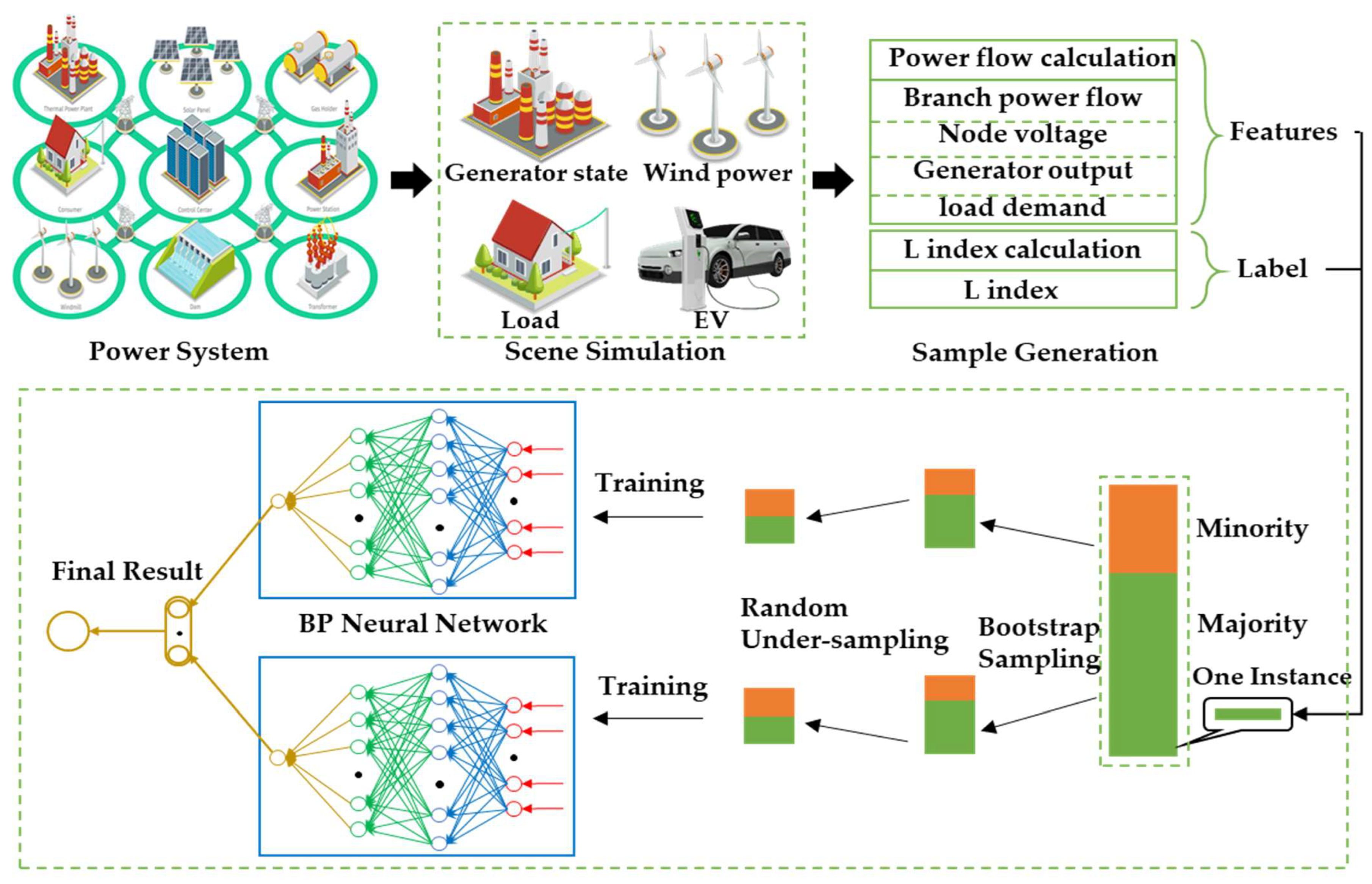
Based on power flow calculation and local voltage stability index calculation, the static voltage stability assessment problem of the power system is treated as a supervised machine learning problem. With the help of the machine learning method, the mapping relationship between the operating state and voltage stability is mined. The idea frame diagram is shown in Figure 4.
In the framework shown in Figure 4, there are mainly four parts: scene generation, sample generation, model building, and model training. The scene simulation is carried out considering the characteristics of the actual operation scene. In addition, the power flow calculation is performed on the simulated scene. The power flow calculation result is a feature variable of the sample corresponding to the scene. Based on the power flow calculation result, the local voltage stability index is calculated too. The index value is the corresponding label value (true value) of the sample in the scene.
The scenario simulation mainly considers the following factors: load demand, generator status, and new energy output power. Specifically, for the load demand, there are heavy load demand and light load demand. For the generator status, the generator does not reach the limit of reactive power and the reactive power of some units reaches the limit. There are two reasons for considering this factor: First, when the generator node transforms into a PQ node, the voltage stability state of the system will change abruptly. Second, the calculation of the L index needs to determine the type of system nodes in advance. When the type of node changes, the L index calculation model needs to be updated. For the output of new energy, the node where the unit is located is regarded as the PQ node. The load side also considers the batch connection to the grid and withdraws from the grid of electric vehicles.
The above factors only consider typical scenarios, so the number of scenarios is limited. Therefore, in the simulation, a mixed simulation of various factors is adopted to expand the number of scenarios. After the scenario simulation is completed, the power flow calculation is carried out for each scenario to obtain the voltage amplitude and phase angle of each node, the active and reactive power output of the generator, and the line power flow. These power flow calculation results and the load demand together constitute the features of samples. The L index corresponds to the features of samples packaged into complete training data. Since the L index can be directly calculated based on the power flow state, it does not require continuous power flow calculation like PV analysis, so the sample collection speed is very fast. The training set, validation set, and test set are randomly selected according to the ratio of 90%, 5%, and 5%.
BP network belongs to supervised learning [27]. In the process of neural network modeling, the selection of activation function, loss function, and the optimization algorithm is required. In the design of hyperparameters, such as the number of hidden layers, the number of neurons in the hidden layer, the number of parallel BP networks, etc., it needs to be set according to specific problems, and these hyperparameters rely more on empirical values.
(1)
Activation function
The activation function is the key to the nonlinear mapping function of the neural network. Common activation functions include Sigmoid, ReLU classes (ReLU, LReLU, RReLU), Tanh and Softmax. Through the nonlinearization of the input data by the above activation function, combined with the deep superposition of the neural network, the fitting of the nonlinear function is realized. In this paper, the LReLU activation function is selected as the activation function of the BP network, because the dead zone of LReLU has a small range. At the same time, LReLU can effectively avoid the problem of gradient disappearance, and also alleviate the problem of neuron death of ReLU, which is beneficial to the neural network. The curve of LReLU is shown in Figure 5. The expression of the LReLU activation function is:
f ( x ) = max { 0.1 x , x }
The domain of the LReLU function is negative infinity to positive infinity. LReLU alleviates the problem of ReLU neuron death and solves the problem that some neurons cannot be activated.
(2)
Loss function
The loss function is used to measure the difference between the output value of the model and the true value of the sample. Through the back-propagation process, the loss function is minimized, the weight of the network is corrected, and the gap between the output value of the model and the true value of the sample is continuously narrowed to achieve network convergence.
For different learning models, such as regression models and classification models, the type of loss function needs to be selected. For the classification model, the cross-entropy loss function is generally used. For the regression model, the mean square error loss function is generally used. In this paper, the problem of voltage stability assessment is defined as a regression problem, so the mean square error function is chosen as the loss function.
E = 1 N i = 1 N ( y i y ^ i ) 2
where E represents the output value of the loss function, N represents the number of samples used in a parameter update process, and y i and y ^ i represent the true value and predicted value of the ith sample label, respectively.
(3)
Optimization algorithm
After completing the construction of the loss function, it is necessary to implement parameter correction through the optimization algorithm. The deep learning optimization algorithm mainly includes the basic optimization algorithm and the adaptive parameter optimization algorithm. The representative algorithm of the basic optimization algorithm is the stochastic gradient descent method, which keeps the learning rate unchanged during the training process. It cannot dynamically adapt to the training requirements. In addition, it is easy to fall into the local optimum point. The representative algorithm of the adaptive parameter optimization algorithm is Adam. The learning rate is gradually attenuated to better adapt to the training requirements as the learning progresses, shorten the training time, and improve the training effect. In this paper, the Adam algorithm [28] is used as the optimization algorithm for network training.
{ m t = μ m t 1 + ( 1 μ ) g t n t = v n t 1 + ( 1 v ) g t 2 m ^ t = m t / ( 1 μ ) n ^ t = n t / ( 1 v ) Δ θ t = m ^ t η g t / n t + ε
In the formula, g t represents the gradient, m t represents the first-order moment estimation of the gradient, n t represents the second-order moment estimation of the gradient, m ^ t and n ^ t represent the corrected values of m t and n t , respectively. μ and v represent the first-order momentum and the second-order momentum, respectively. Momentum coefficient, ε means avoiding smoothing terms with 0 denominators, η means learning rate. The standard settings for μ and v are 0.9 and 0.999, respectively, and the default value for η is 0.001. A satisfactory training effect can be obtained by applying this set of hyperparameters during the training process, and no special adjustment is generally required.

5. Results

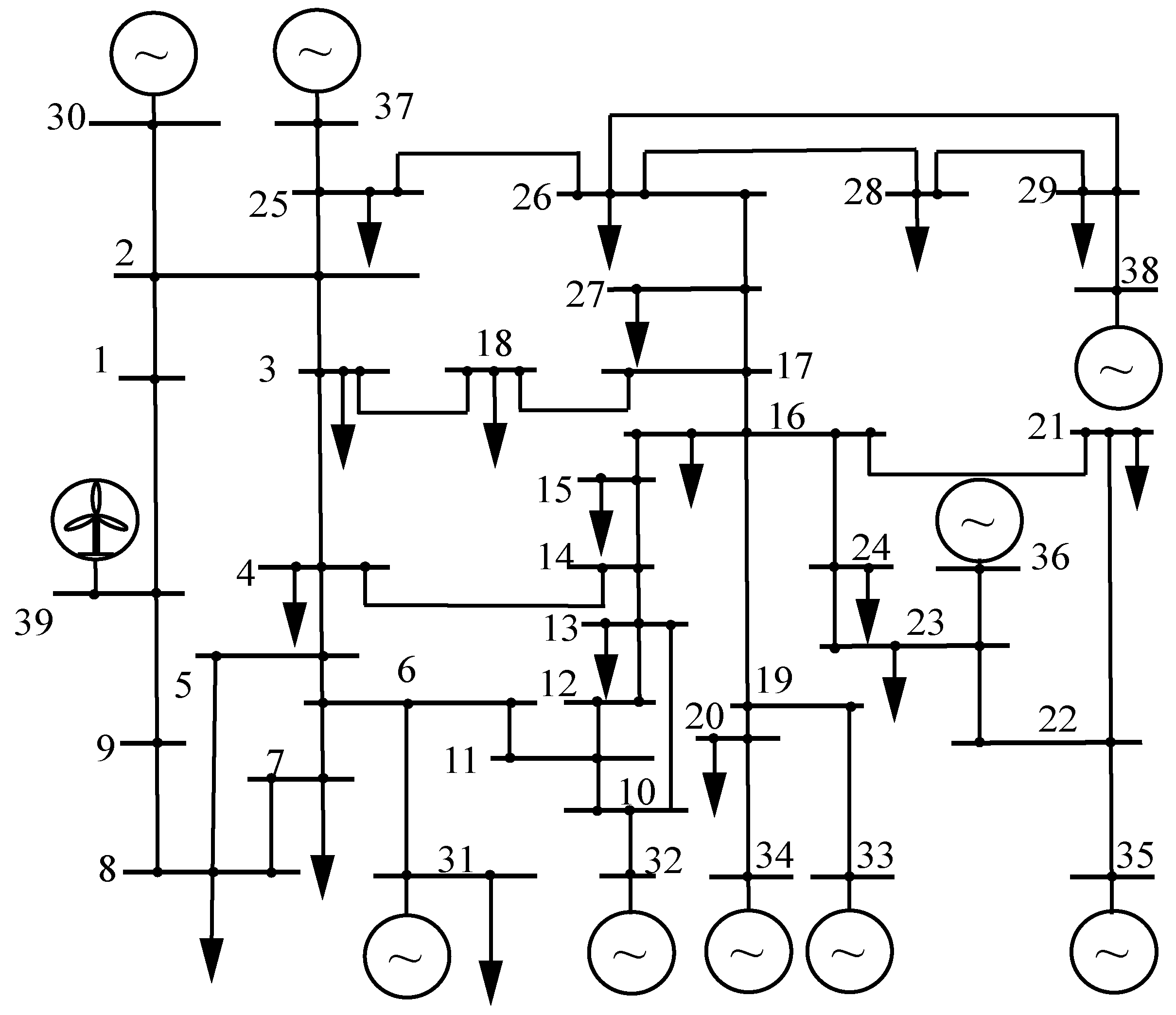
To verify the effectiveness of the proposed model, the modified IEEE39 system case is taken as an example, as shown in Figure 6. The IEEE39 system [29] has 39 nodes, 19 load nodes, 10 thermal power units, and 46 branches (including transformers) with the following modifications: replacing the thermal power generator on bus-39 with wind turbines with a capacity of 650 MVA and removing the load of bus-39.
The neural network model is built based on the Pytorch framework, and the power system simulation is performed based on the PSSE simulation platform. An analysis is developed from the perspectives of model training time, mean square error (MSE), and mean absolute percentage error (MAPE).
In machine learning, MSE is generally used as the error of model training, and it is used as the objective function to update the parameters. The expression of MSE is shown in Formula (17):
MSE = 1 n i = 1 n ( y i y i ) 2
where y i is the predicted value of the ith sample, and y i is the true value of the ith sample. The advantage of MSE is to amplify extreme errors and avoid huge deviations in the model. The disadvantage is that it is not intuitive and it is difficult to explain its meaning after squaring.
In order to intuitively reflect the difference between the actual value and the predicted value, there is MAPE, which is expressed as Formula (18):
MAPE = 1 n i = 1 n | y i y i | y i
The value of MAPE is intuitive and has a clear meaning, but when the actual value is very small, it is easy to produce misleading information. Therefore, MAPE is generally not used for the loss function of regression problems with small real values, but it can be used as a more intuitive method to measure the model error.
In summary, MSE is used to evaluate the overall performance of the model, and MAPE is used to evaluate the performance of the model on batch instances.
The training time of different methods and the MSE and MAPE error of each method on the test set are shown in Table 2.
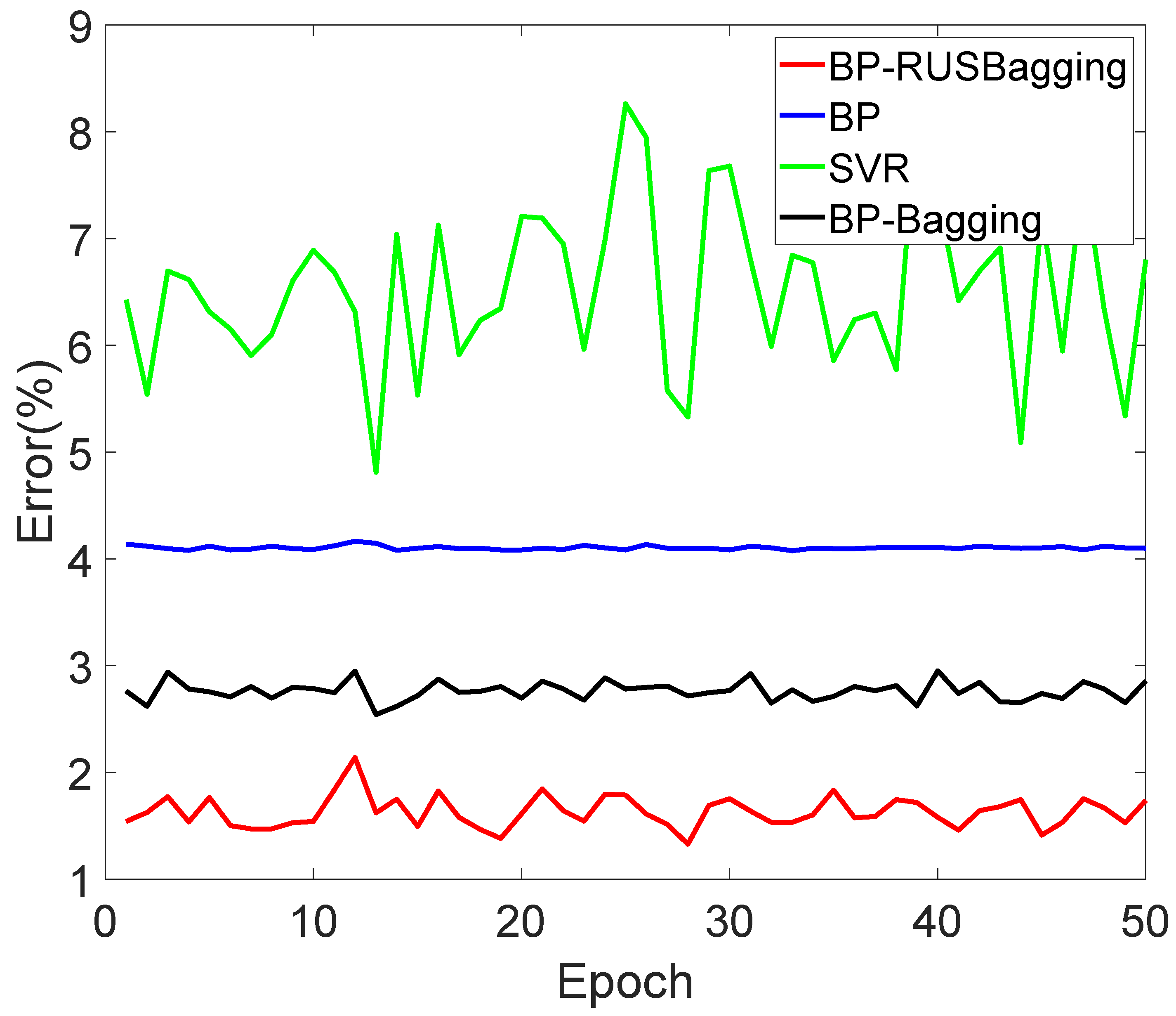
SVR stands for support vector regression. The test set is divided into multiple batches of data, and each batch of data is calculated to obtain the batch MAPE index and plot the results, as shown in Figure 7.
As shown in Figure 7, the errors of the four methods on the test set are all small, and the advantage of method 1 is not obvious. This is because the test set is also a class-imbalanced data set, so the advantage of the under-sampling method is not prominent on the whole test set.
To further illustrate the applicability of the proposed method to the class imbalance problem, the minority class samples in the test set are screened out, and then four methods are used for comparison based on the minority test set. The results are shown in Table 3.
As shown in Figure 8, on the screened test set, the proposed method has obvious advantages over other methods. It has a lower error on minority class samples. Compared with methods 3 and 4, method 2 also shows the adaptability to the class imbalance problem to a certain extent. This should be credited to the bagging framework.

6. Conclusions

The comparative analysis proves that the proposed static voltage stability assessment method not only has high accuracy, strong adaptability, and short modeling time but also has the following advantages:
(1)
In the sample preparation stage, various operating scenarios such as load demand, new energy output power, and EV status were considered, which greatly improved the scenario applicability of the model.
(2)
Defining the static voltage stability assessment problem as a regression problem of machine learning, which essentially improves the model assessment accuracy, provides voltage stability information with a quantitative index, and helps grid operators to better observe the grid state.
(3)
Using the random under-sampling bagging framework provides a method to solve the problem of imbalanced data in the field of power system operating, which comprehensively improves the accuracy of the model.

Author Contributions

Conceptualization, P.Z. and J.W.; methodology, P.Z. and Z.L.; software, Z.Z. and Z.L.; validation, Z.Z. and J.W.; formal analysis, P.Z. and Z.L.; investigation, J.W. and Z.L.; resources, P.Z.; data curation, Z.Z. and J.W.; writing—original draft preparation, Z.Z.; writing—review and editing, P.Z. and J.W.; visualization, Z.Z.; supervision, P.Z.; project administration, P.Z.; funding acquisition, Z.L. All authors have read and agreed to the published version of the manuscript.

Funding

This research was funded by National Nature Science Foundation of China, grant number 52107068.

Data Availability Statement

Not applicable.

Acknowledgments

Not applicable.

Conflicts of Interest

The authors declare no conflict of interest.

References

  1. Kundur, P. Power System Stability and Control; McGraw-Hill: New York, NY, USA, 1993. [Google Scholar]
  2. Van Cutsem, T.; Vournas, C. Voltage Stability of Electric Power Systems; Kluwer: Cambridge, UK, 1998. [Google Scholar]
  3. Srivastava, L.; Singh, S.N.; Sharma, J. Estimation of loadability margin using parallel self-organizing hierarchical neural network. Comput. Electr. Eng. 2000, 26, 151–167. [Google Scholar] [CrossRef]
  4. Suganyadevi, M.V.; Babulal, C.K. Online Voltage Stability Assessment of Power System by Comparing Voltage Stability Indices and Extreme Learning Machine; Springer: Berlin, Germany, 2013. [Google Scholar]
  5. Qiang, W.; Hao, C.; Lian, L. Static Voltage Stability Margin Prediction Based on Natural Gradient Boosting and Its Influencing Factors Analysis. In Proceedings of the CSU-EPSA, Prague, Czech Republic, 23–25 June 2022; pp. 1–9. [Google Scholar]
  6. Ghiocel, S.G.; Chow, J.H. A Power Flow Method Using a New Bus Type for Computing Steady-State Voltage Stability Margins. IEEE Trans. Power Syst. 2014, 29, 958–965. [Google Scholar] [CrossRef]
  7. Luo, F.; Dong, Z.Y.; Chen, G.; Xu, Y.; Meng, K.; Chen, Y.Y. Advanced pattern discovery-based fuzzy classification method for power system dynamic security assessment. IEEE Trans. Ind. Informat. 2015, 11, 416–426. [Google Scholar] [CrossRef]
  8. Gholami, M.; Sanjari, M.J.; Safari, M.; Akbari, M.; Kamali, M.R. Static security assessment of power systems: A review. Int. Trans. Electr. Energy Syst. 2020, 30, e12432. [Google Scholar] [CrossRef]
  9. Liu, S.; Liu, L.; Yang, N.; Mao, D.; Shi, R. A data-driven approach for online dynamic security assessment with spatial-temporal dynamic visualization using random bits forest. Int. J. Electr. Power Energy Syst. 2021, 124, 106316. [Google Scholar] [CrossRef]
  10. Ding, C.; Zhang, P.; Meng, X.; Li, W.; Wang, Y. Online Evaluation on Static Voltage Stability Margin Based on Classification and Regression Tree Algorithm. Proc. CSU-EPSA 2020, 32, 93–100. [Google Scholar]
  11. Wenqing, L.; Qingwu, G.; Chunhui, G.; Liu, H.; Liu, W.; Liuchuang, W.U. Transient voltage stability evaluation based on feature and convolutional neural network. Eng. J. Wuhan Univ. 2019, 52, 815–823. [Google Scholar]
  12. Xiurui, L.; Daowei, L.; Hongying, Y. Data-Driven Situation Assessment of Power System Static Voltage Stability. Electr. Power Constr. 2020, 41, 126–132. [Google Scholar]
  13. Zhu, L.; Lu, C.; Dong, Z.Y. Imbalance learning machine-based power system short-term voltage stability assessment. IEEE Trans. Ind. Inform. 2017, 13, 2533–2543. [Google Scholar] [CrossRef]
  14. Johnson, J.M.; Khoshgoftaar, T.M. Survey on deep learning with class imbalance. J. Big Data 2019, 6, 1–54. [Google Scholar] [CrossRef]
  15. Li, Y.; Zhang, M.; Chen, C. A Deep-Learning intelligent system incorporating data augmentation for Short-Term voltage stability assessment of power systems. Appl. Energy 2022, 308, 118347. [Google Scholar] [CrossRef]
  16. Haixiang, G.; Yijing, L.; Shang, J.; Mingyun, G.; Yuanyue, H.; Bing, G. Learning from class-imbalanced data: Review of methods and applications. Expert Syst. Appl. 2017, 73, 220–239. [Google Scholar] [CrossRef]
  17. Malave, N.; Nimkar, A.V. A survey on effects of class imbalance in data pre-processing stage of the classification problem. Int. J. Comput. Syst. Eng. 2020, 6, 63–75. [Google Scholar] [CrossRef]
  18. Khan, S.H.; Hayat, M.; Bennamoun, M.; Sohel, F.; Togneri, R. Cost-sensitive learning of deep feature representations from imbalanced data. IEEE Trans. Neural Netw. Learn. Syst. 2017, 29, 3573–3587. [Google Scholar] [PubMed]
  19. Rao, N.A.; Vijaya, P.; Kowsalya, M. Voltage stability indices for stability assessment: A review. Int. J. Ambient. Energy 2021, 42, 829–845. [Google Scholar]
  20. Salama, H.S.; Vokony, I. Voltage stability indices–A comparison and a review. Comput. Electr. Eng. 2022, 98, 107743. [Google Scholar] [CrossRef]
  21. Kessel, P.; Glavitsch, H. Estimating the Voltage Stability of a Power System. IEEE Trans. Power Deliv. 2007, 1, 346–354. [Google Scholar] [CrossRef]
  22. Wei, W.; Xu, Y. Deterministic convergence of an online gradient method for neural networks. J. Comput. Appl. Math. 2002, 144, 335–347. [Google Scholar]
  23. Zhang, L.; Wang, F.; Sun, T.; Xu, B. A constrained optimization method based on BP neural network. Neural Comput. Appl. 2018, 29, 413–421. [Google Scholar] [CrossRef]
  24. Shi, X.; Xu, G.; Shen, F. Solving the data imbalance problem of P300 detection via random under-sampling bagging SVMs. In Proceedings of the 2015 International Joint Conference on Neural Networks, Killarney, Ireland, 12–17 July 2015; pp. 1–5. [Google Scholar]
  25. Błaszczyński, J.; Stefanowski, J. Actively balanced bagging for imbalanced data. In Proceedings of the International Symposium on Methodologies for Intelligent Systems, Graz, Austria, 23–25 September 2017; pp. 271–281. [Google Scholar]
  26. Bühlmann, P. Bagging, boosting and ensemble methods. In Handbook of Computational Statistics; Springer: Berlin, Germany, 2012; pp. 985–1022. [Google Scholar]
  27. Goodfellow, I.; Bengio, Y.; Courville, A. Deep Learning. MIT Press: Cambridge, UK, 2016. [Google Scholar]
  28. Guan, N.; Lei, S.; Yang, C.; Xu, W.; Zhang, M. Delay Compensated Asynchronous Adam Algorithm for Deep Neural Networks. In Proceedings of the 2017 IEEE International Symposium on Parallel and Distributed Processing with Applications and 2017 IEEE International Conference on Ubiquitous Computing and Communications (ISPA/IUCC), Guangzhou, China, 12–15 December 2017; IEEE: Piscataway, NJ, USA, 2017. [Google Scholar]
  29. Sriyanyong, P.; Song, Y.H. Unit commitment using particle swarm optimization combined with Lagrange relaxation. In Proceedings of the Power Engineering Society General Meeting, San Francisco, CA, USA, 16 June 2005. [Google Scholar]
Figure 1. Structure diagram of typical BP neural network.
Processes 10 01938 g001
Figure 2. Schematic diagram of random under-sampling.
Processes 10 01938 g002
Figure 3. Schematic diagram of the random under-sampling bagging method.
Processes 10 01938 g003
Figure 4. The framework for static VSA of power system based on RUSBagging.
Processes 10 01938 g004
Figure 5. The curve of LReLU.
Processes 10 01938 g005
Figure 6. Modified IEEE 39 bus system.
Processes 10 01938 g006
Figure 7. MAPE results of each method on the whole test set.
Processes 10 01938 g007
Figure 8. MAPE results of each method on the minority test set.
Processes 10 01938 g008
Table 1. Algorithm of the random under-sampling bagging method.
Input: dataset D = { ( x 1 , y 1 ) , ( x 2 , y 2 ) , , ( x n , y n ) } , weak learner algorithm, number of weak learner M
For i = 1, 2, …, M:
        Using the bootstrap sampling method on the dataset D to generate a subsampled set D i
        Using the random under-sampling method on the dataset D i to generate a balanced subsample set D i
        Training the ith weak learner G i ( x ) with a balanced subsample set D i
End
Output: the final model
Table 2. Comparison of the performance of different methods on the whole test set.
NumMethodsTrain-Time/sMSEMAPE
1BP-RUSBagging312.446.0252 × 10−70.0011
2BP-Bagging290.354.7632 × 10−70.0014
3BP213.542.2391 × 10−60.0018
4SVR564.219.3797 × 10−60.0022
Table 3. Comparison of the performance of different methods on the minority test set.
NumMethodsTrain-Time/sMSEMAPE
1BP-RUSBagging312.441.7763 × 10−50.0167
2BP-Bagging290.358.1022 × 10−50.0284
3BP213.542.2391 × 10−40.0411
4SVR564.211.4397 × 10−30.0622
Publisher’s Note: MDPI stays neutral with regard to jurisdictional claims in published maps and institutional affiliations.

