Dynamic Load Redistribution of Power CPS Based on Comprehensive Index of Coupling Node Pairs

Abstract

The adoption of power cyber physical systems (Power CPS) is becoming more and more widespread, and as risk spreads, cascading failures of overload behavior can lead to the collapse of individual or entire networks, becoming a major threat to the network security. Taking the power CPS coupling node pair as the starting point, this paper establishes the comprehensive indicators characterizing the importance and vulnerability of the coupled node pair, based on the idea of intrusion tolerance, when the cyber side is faulted by the network attack, the system actively carries out reasonable and effective dynamic load redistribution based on the indicators updated after each round of cascading, thereby inhibiting the spread of risk, reducing system losses, and improving survivability. The above theory is simulated on the IEEE 30-bus system and concludes that the proposed load redistribution strategy can effectively reduce the loss of the system after attacks.

1. Introduction

The smart grid is a typical cyber-physical system (CPS) [1] with a large number of measurements, control units, advanced information, and communication technologies. These technologies make the power system operate more stably and safely, but also exacerbate the system’s vulnerability. Due to cyber and physical network coupling, cross-space cascade failures can carry the risk from one side to the other. For example, a major cause of the North American blackout in 2003 was a state estimation failure in the information system, when an unexposed failure occurred on the physical side at the same time [2].

The currently available techniques for preventing and mitigating the propagation of cascading failures can be divided into three categories [3]: attack prevention techniques, attack detection techniques, and intrusion tolerance techniques. Since the currently available detection and defense means are not perfect and the system is inevitably compromised, the application of the third approach is gaining attention in order to maintain the observability and controllability of the system as much as possible [4]. Ref. [5] investigated the resistance of power systems to attack under an average redistribution strategy. Ref. [6] used the WPA-PFRA approach to redistribute the currents in the network. However, the above two papers consider only the power system and do not address the cyber side. Ref. [7] described the redundancy characteristics of nodes based on the “load-capacity” model using overload states and failure probabilities for load redistribution, but this method is only applied in single-layer networks. Ref. [8] used a local nearest neighbor weighted assignment strategy to analyze cascading failures in complex networks. A load redistribution model with an adjustable redistribution range and redistribution uniformity is proposed in [9]. Ref. [10] aimed to reduce the critical threshold and effectively improve the robustness of the network, allocating based on the maximum available capacity of the remaining nodes. However, there are many problems in the above papers, such as not considering both the structural and functional characteristics of the system, or not considering the cyber side and the physical side organically.

Therefore, in this paper, based on the third intrusion-tolerant solution, load redistribution under cascade failure is carried out in two steps as follows:

(1)

The integrated importance and vulnerability indexes of node pairs are established by combining the functional characteristics of the system.

(2)

Based on the update of indicators, dynamic load redistribution of information flow and power flow of failed nodes is carried out in the process of cascading failure, so that the fault can be terminated quickly.

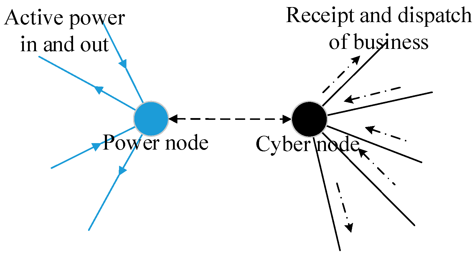
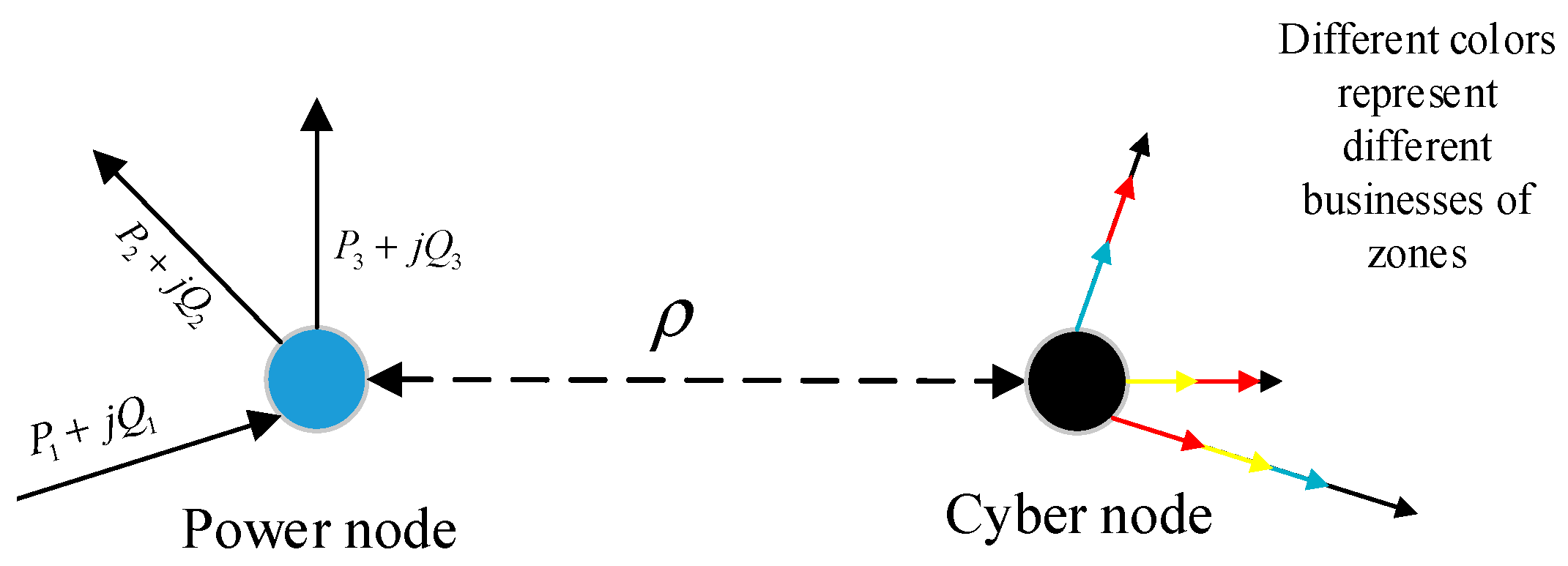
2. The Comprehensive Characteristics of the Coupling Node Pair

In this paper, the degree-betweenness coupling interface strategy [11] takes a pair of coupled power nodes and cyber nodes as a whole. The coupling part of the two subnetworks within the power CPS is the key link, which includes the corresponding power grid node, cyber network node, and cyber-physical connection edge.

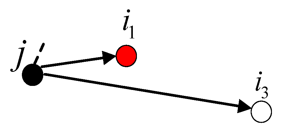
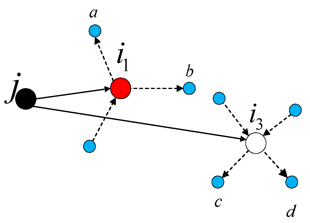
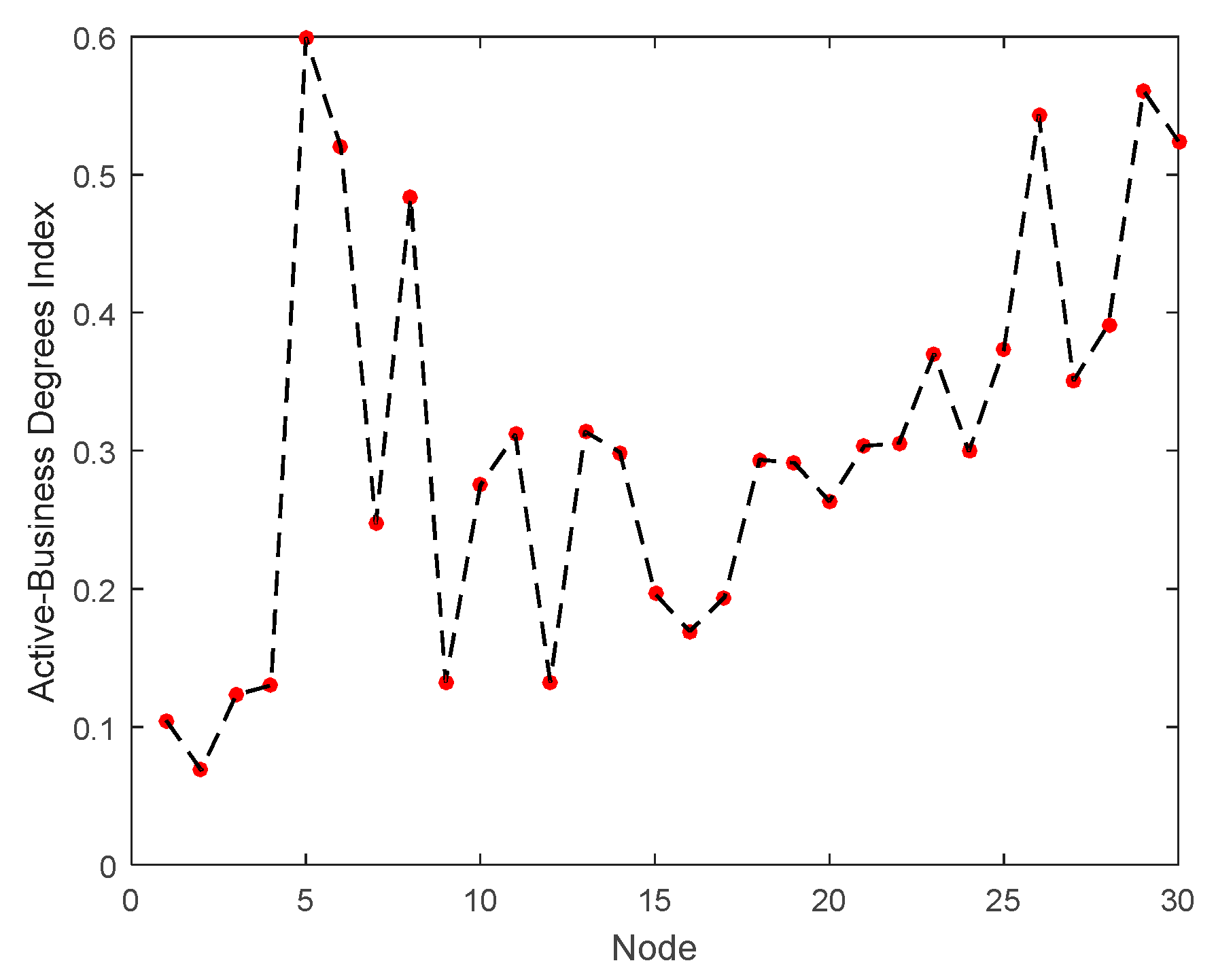
2.1. Active-Business Degree Index

A large amount of literature shows that the number of node degrees alone does not reflect the importance of nodes or node pairs in the system.

As shown in Figure 1, on the power side, each power node is connected to multiple power lines, and there is power inflow or outflow on each node. The importance of each power node is evaluated by combining the magnitude of the power flow and its flow direction. On the cyber side, each cyber node is connected to multiple links, and each link carries one or more different services, and different services have different importance. So, the structural characteristics are combined with the business characteristics on the cyber side to quantify the cyber node importance.

The importance of the power side node i can be characterized as I_pi:

$$I_{pi}=\frac{k_{ii}{\displaystyle \sum p_{ii}}+k_{io}{\displaystyle \sum p_{io}}}{<k_p{>}^2}$$

(1)

where the average degree value of the power network node is represented as $<k_p>$; $k_{ii}$ is the number of active lines injected into the i node, and ${\displaystyle \sum p_{ii}}$ is the input active value of the i node; $k_{io}$ is the number of active lines flowing out of the i node, and ${\displaystyle \sum p_{io}}$ is the output active value of the i node.

In order to simplify the calculation, the average importance of the service is taken according to the security partition [12], that is, the importance of the security zone I to IV is 0.835, 0.41, 0.315, 0.223, respectively. The cyber-side node service importance formula is as follows:

$$I_{ci}={\displaystyle \sum _{a=1}^n{\displaystyle \sum _{l=1}^K{b}_{al}{h}_{al}}}$$

(2)

where b_xl is the importance of class x service on the service link l connected by node i, h_xl is the number of class x services on the service link l, and K is the collection of adjacent links of node i. The service importance is evaluated according to the latency, bit error rate, real-time, reliability, etc. [13].

Therefore, the active-business degree of the coupled node pair can be established according to the power node active degree and the service importance of the cyber node, which is used to characterize the importance of the node in the whole network:

$$I_{vi}=(1-{\beta }_{cp})I_{pi}^{\prime }+{\beta }_{cp}{I}_{ci}^{\prime }$$

(3)

where ${\beta }_{cp}$ is the weight allocation coefficient for importance, $I_{pi}^{\prime }$ and $I_{ci}^{\prime }$ are normalized subnet node importance metrics, respectively.

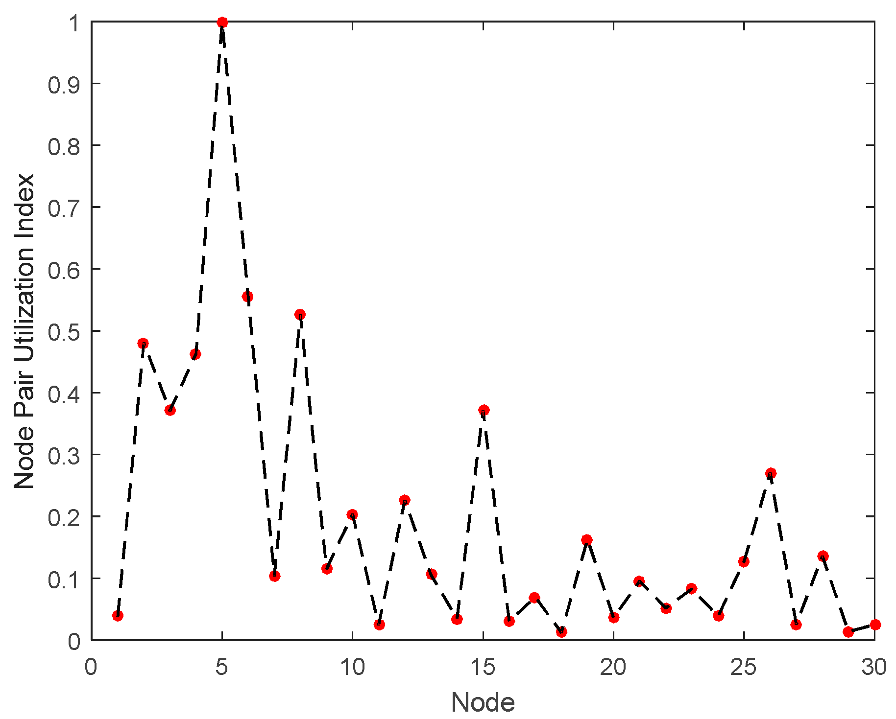
2.2. Node Pair Utilization Index

Coupled networks in power systems have proven to be more vulnerable than single-layer networks [14].

As shown in Figure 2, on the power side, the ratio of the power transmitted on the line to the upper limit of its capacity is defined as the utilization rate of the transmission line [15]. The power nodes are connected by transmission lines, so the node utilization rate is defined, which is the ratio of the power flowing through the node to the capacity of the node. The higher the utilization, the easier it is for the node to approach the limit value when the load increases. Therefore, the power node utilization rate can be defined as:

$$U_{pi}=\frac{{\displaystyle \sum (\sqrt{P{F}_{li}^2+Q{F}_{li}^2}+\sqrt{P{T}_{li}^2+Q{T}_{li}^2})}}{2C_{pi}}$$

(4)

where li is the adjacent line of node i. $P{F}_{li}$ and $Q{F}_{li}$ are the active and reactive power at the outflow end of line li, respectively. $P{T}_{li}$ and $Q{T}_{li}$ are the active and reactive power at the receiving end of the line li, respectively.

For a power-side node, the one delivering power to the node is called the parent node, and the one receiving power from the node is called the child node, which is shown in Figure 3 below.

The more children nodes a node has, the more risk will be passed on to that node, making it more vulnerable, and conversely, the more parent nodes it has, the more risk it can be to help share. Therefore, the vulnerability indicator of the power side can be defined as:

$${\eta }_{pi}=U_{pi}\text{·}{e}^{k_{io}-k_{ii}}$$

(5)

The cyber side adopts a variety of technologies for defense, such as firewalls, identity authentication, VPN, intrusion detection, isolation, encryption, and other means [16]. Therefore, the threat degree formula for the cyber-side coupling node can be defined as follows:

$${\eta }_{ci}=f_{uti}{I}_{dis}{k}_i\cdot \frac{C_i}{C_{ci}}$$

(6)

Among them, $f_{uti}$ represents the vulnerability utilization of node i on the cyber side; $I_{dis}$ indicates the degree of vulnerability distribution; k_i is the degree of node i. The security zone where the vulnerability is located is used as the main basis to assess the vulnerability utilization and vulnerability distribution impact degree. After a comprehensive statistical measurement [16]. it can be seen that the threatened degree $f_{uti}\cdot I_{dis}$ of vulnerabilities in each security zone is shown in

Table 1. Risk levels for each security partition.

Security Zone	Score	Risk Levels
I	4	High
II	3	Medium
III	4	High
IV	2	Low

:

Therefore, the comprehensive vulnerability indexes of the coupling node pair based on utilization can be established as follows:

$${\eta }_{vi}=\rho ({\gamma }_{cp}{\eta }_{{}_{pi}}^{\prime }+(1-{\gamma }_{cp}){\eta }_{{}_{ci}}^{\prime })$$

(7)

Further, ρ is the probability of inter-network failure (0 < ρ < 1), characterizing the odds of risk spreading across space, and ${\gamma }_{cp}$ is the vulnerability weight coefficient, and ${\eta }_{{}_{pi}}^{\prime }$ and ${\eta }_{{}_{ci}}^{\prime }$ are normalized subnet node vulnerability metrics, respectively.

3. Power CPS Risk Propagation Considering Load Redistribution

The work of the actual power system shows that in order to ensure real-time observation of the grid operation, cyber-side nodes are often stocked with a large number of UPS power supplies, and the failure of a power node does not directly affect the normal operation of the cyber network [17].

When considering the load-capacity model, the survival conditions of the coupled nodes change [18] and only fail when the node exceeds its maximum capacity. A distribution strategy that considers only the centrality of nodes can invalidate nodes in a central position due to a larger distribution load [19]. At present, the information-focused routing strategies commonly used are: routing based on the shortest path, even distribution policies, etc. [20], and there are few articles on load redistribution by establishing indicators.

3.1. Initial Load and Capacity of CPS Nodes

In a subnetwork, when a node fails, the load on that node is redistributed to the other nodes. Cascade failure occurs if the node capacity is exceeded.

3.1.1. Power Side

On the power side, the power flow consists of active and reactive components and is calculated in terms of apparent power:

$$S_l={\displaystyle \sum _{\begin{array}{l}j\ne i\\ j=1\end{array}}^n{S}_{ij}=}{\displaystyle \sum _{\begin{array}{l}j\ne i\\ j=1\end{array}}^n{V}_i{y}_{ij}^{*}\left(V_i^{*}-V_j^{*}\right)=}{V}_i{\left(YV\right)}_i^{*}$$

(8)

In general, due to the existence of line impedance, the voltage of the node at the sending power end and the node at the receiving power end on the same line are different, resulting in different apparent power on both sides of the line. Thus, the power flow of the line can be defined as:

$$|L_{li}(0)|=\frac{\left|S_{Fl}\right|+\left|S_{Tl}\right|}{2}$$

(9)

where $|L_{li}(0)|$ is the initial average power flow on line l, $\left|S_{Fl}\right|$ is the apparent power at the sending-power end of the line, and $\left|S_{Tl}\right|$ is the apparent power at the receiving-power end of the line.

Expand it to get:

$$|L_{li}(0)|=\frac{\sqrt{P{F}_{li}^2+Q{F}_{li}^2}+\sqrt{P{T}_{li}^2+Q{T}_{li}^2}}{2}$$

(10)

Then, the initial load of node i is the sum of the initial loads of all connected neighboring lines:

$$L_{pi}(0)={\displaystyle \sum _{li\in \mathsf{\Gamma }i}{L}_{li}(0)}$$

(11)

where $L_{pi}(0)$ is the initial total load of node i.

Power node capacity is proportional to the initial load:

$$C_{pi}=(1+{\alpha }_p)L_{pi}(0)$$

(12)

where ${\alpha }_p$ is the power-side capacity margin factor.

3.1.2. Cyber Side

The initial amount of information of cyber node i can be defined as:

$$L_{ci}(0)=n_{\mathrm{Ⅰ}}^{{\tau }_{\mathrm{Ⅰ}}}+n_{\mathrm{Ⅱ}}^{{\tau }_{\mathrm{Ⅱ}}}+n_{\mathrm{Ⅲ}}^{{\tau }_{\mathrm{Ⅲ}}}+n_{\mathrm{Ⅳ}}^{{\tau }_{\mathrm{Ⅳ}}}$$

(13)

Among them, n_I, n_II, n_III, and n_IV are the traffic volume belonging to the four security zones carried on the i node, τ_I, τ_II, τ_III, and τ_IV are the load adjustable parameters to control the load intensity of different safety zones of the node i.

The maximum capacity of an information node is related to the initial amount of information as follows [21]:

$$C_{ci}=(1+{\alpha }_c)L_{ci}(0)$$

(14)

where ${\alpha }_c$ is the capacity margin factor of cyber nodes.

The constraints for cyber nodes and power nodes to operate normally without exceeding the capacity limit are:

$$\{\begin{array}{l}0<L_{pi}\left(0\right)\le C_{pi}\\ 0<L_{ci}\left(0\right)\le C_{ci}\end{array}$$

(15)

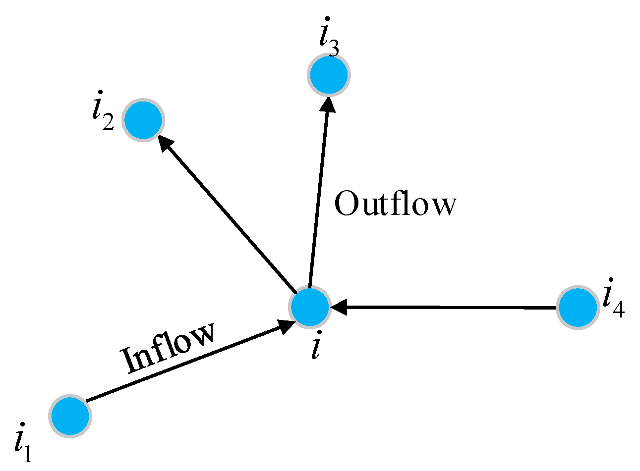
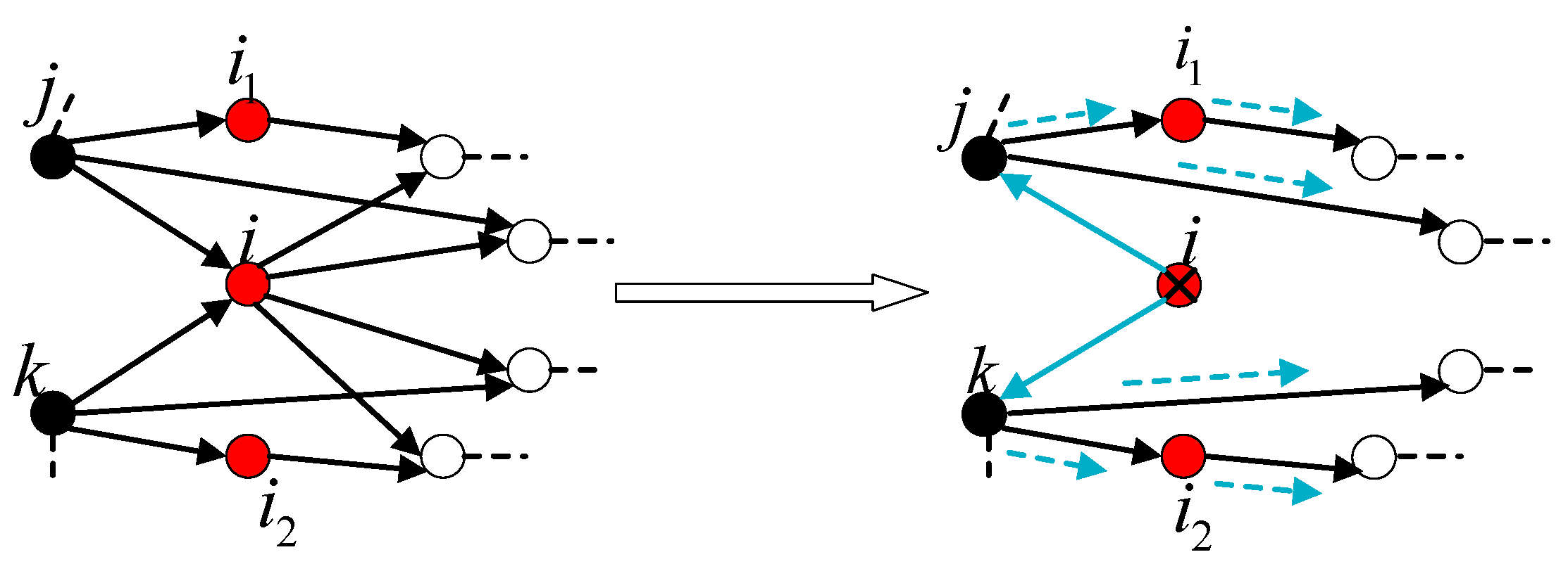
3.2. Subnetwork Load Reallocation

This paper adopts the dynamic allocation strategy of nearest neighbor selection based on indicators, and processes the risk propagation at each stage in two rounds, making the best choice under the current situation and terminating the cascade failure as soon as possible.

3.2.1. Cyber Network Load Reallocation

The best routing of the cyber network itself may not be optimal for the power system, so optimal routing in favor of the power system should be established to ensure the accessibility of critical information flows [22]:

(1)

The first round of redistribution on the information side

When multiple nodes fail at t-time, the nodes with relatively high importance in the front row are prioritized for load redistribution. The specific allocation steps are as follows:

The first stage of load redistribution of a single failed node v_i is carried out, and the full load of the v_i node is distributed to all neighbor nodes.

For the information-side failure node v_i, the load is zeroed, that is, L_i = 0, the relevant row and column elements are zeroed in the coupling adjacency matrix, and the neighbor node set of v_i is collected and recorded while removing the line connected to the v_i node. For multiple neighbor nodes of node v_i, their comprehensive vulnerability is sorted according to at the t + 1 moment, one of v_i’s neighbor nodes v_j will be allocated to a certain proportion of the load, then v_i reassigned to v_j. The load increment is:

$$L_{ij}(t+1)=L_i(t)\cdot \frac{\eta (v_j)}{{\displaystyle \sum _{n\in {\mathsf{\Gamma }}_i}\eta (v_n)}}$$

(16)

where $L_{ij}(t+1)$ is the load reallocated to node j at the moment of t + 1, and $L_i(t)$ is the load before node i fails; $\eta (v_j)$ is the comprehensive vulnerability index of node j, and $\frac{\eta (v_j)}{{\displaystyle \sum _{n\in {\mathsf{\Gamma }}_i}\eta (v_n)}}$ is the weight assigned to the load, following the node parameters after each round of redistribution; ${\mathsf{\Gamma }}_i$ is the set of neighbor nodes of node i.

If multiple neighbor nodes of node j fail, then all failed neighbor nodes may redistribute load to j, and the load increment on node j at the t + 1 moment is:

$$\mathsf{\Delta }{L}_j(t+1)={\displaystyle \sum _{i\in {\mathsf{\Gamma }}_j}{L}_{ij}(t+1)}$$

(17)

where ${\mathsf{\Gamma }}_j$ is the set of failed neighbor nodes for node j.

The total load on node j is:

$$L_j(t+1)=\mathsf{\Delta }{L}_j(t+1)+L_j(t)$$

(18)

where $L_j(t)$ is the load of node j at t-time.

(2)

The second round of redistribution on the information side

The first round of redistribution ends with updating the loads and metrics for all changed nodes. At this time, the status of the remaining nodes of the information network is divided into three cases:

(1)

Normal state, can operate normally;

(2)

In the overload state, but not exceeding the capacity, it can maintain normal operation in the short term, but it needs to be processed as soon as possible;

(3)

Exceeding the maximum capacity and being in a failed state requires a new round of load redistribution.

No processing is required when the node is in the first case. Repeat the actions in the first round when the third case occurs. In the second case, the overload of the information node will cause the throughput of the node to mismatch, and the system will gradually become congested. During this time, the excess portion of the load can be redistributed again.

The steps for the second round of load redistribution are:

Step 1: Collect nodes that are in an overloaded state and newly failed with their load.

Step 2: Redistribute the excess load of the overloaded nodes, and redistribute the entire load of the nodes that exceed the capacity according to the method of the first round.

Step 3: Calculate the load amount of all nodes after this round of load redistribution, if the case of no node overload is satisfied (1), no operation is required, and the cascade failure ends; if (2) or (3), return to step 1.

Constraints satisfied: $L_j(t+1)\le C_{cj}$. $C_{cj}$ is the capacity of node j. When $L_j(t+1)>C_{cj}$, it means that the load of node j exceeds its capacity, and the cyber node j fails, causing a new load redistribution.

3.2.2. Power Grid Load Redistribution

After the cascade of the information side is completed, all the failed information nodes are counted and the corresponding failure nodes of the coupling power side are found, and the first round of redistribution of the power side is carried out.

Considering the node heterogeneity of the power side, it can be divided into three types of nodes, namely the generator node, the load node, and the intermediate node, which constitute the power side directed topology network. It is divided into two steps to suppress the cascade fault propagation on the power side, first adjust the generator output according to the real-time operation situation for power flow adjustment, and if the power flow has not converged, the partial load is removed.

(1)

The first round of redistribution on the power side

As can be seen from Figure 4, after the failure of the i node, the recovered power flow is all returned to the j node and the k node. When the system is operating normally, power conservation is met:

$$L_{ji}+L_{ki}=\mathsf{\Delta }{L}_i+L_{io}$$

(19)

where $L_{ji}$ and $L_{ki}$ are the power flowing to the i node, $\mathsf{\Delta }{L}_i$ is the power consumed by the node i, and $L_{io}$ is the power flowing out of the i node.

When node i fails, the lines directly connected around it will be cut. The power carried by nodes j and k at this time is:

$$\{\begin{array}{l}{L}_j=L_{jo}+L_{ji}+{\displaystyle \sum L_{jloss}}\\ L_k=L_{ko}+L_{ki}+{\displaystyle \sum L_{kloss}}\end{array}$$

(20)

If the parent node of the i node is not a generator node, continue to go back up to find the nearest generator.

When traced back to generator nodes j and k, the power flow is redistributed according to the sum of the recovered tide and the original tide according to the real-time redundancy of the node. Taking apart the j node in the above figure, it is connected to the i₁ and i₃ nodes and other child nodes, in addition to the i node.

As shown in Figure 5, at the generator node, according to the capacity redundancy allocation strategy, the power flow allocated to the i₁ node is:

$$\mathsf{\Delta }{L}_{j{i}_1}=\mathsf{\Delta }{L}_j\frac{C_{i_1}-L_{i_1}}{{\displaystyle \sum (C_{jx}-L_{jx})}}$$

(21)

The tide reassigned to the i₃ node is:

$$\mathsf{\Delta }{L}_{j{i}_3}=\mathsf{\Delta }{L}_j\frac{C_{i_3}-L_{i_3}}{{\displaystyle \sum (C_{jx}-L_{jx})}}$$

(22)

where j_x denotes the neighbor node of node j.

The other failed nodes in the first round on the power side operate as above.

(2)

The second round of redistribution on the power side

The first round of cascading failure under the power flow redistribution has ended, update the adjacency matrix and node pair indicators. At this time, the generator node has begun to readjust the power flow. If the final power flow does not converge, then take the way to reduce the load to make the tide converge. The subsequent redistribution process is also carried out according to the established node-to-synthetic vulnerability indicator.

As shown in Figure 6, the new loads allocated to i₁ and i₃ in the first round are $\mathsf{\Delta }{L}_{ji1}$ and $\mathsf{\Delta }{L}_{ji3}$, and the child nodes are a, b, c, and d. Similar to the information side, according to the updated comprehensive importance indicator $I_i=\left[I_1,I_2,I_3,\cdots ,I_n\right]$, the excess tide of the node with high importance is first redistributed. Unlike the information side, only child nodes on the power side receive the power flow. The child nodes of i₁ are a and b, according to the comprehensive vulnerability indicator ${\eta }_i=\left[{\eta }_1,{\eta }_2,{\eta }_3,\cdots ,{\eta }_n\right]$, where the tide that node a needs to receive is:

$$\mathsf{\Delta }{L}_{a,red}=(\mathsf{\Delta }{L}_{ji1}+L_{i1}-C_{i1})\cdot \frac{{\eta }_a}{{\displaystyle \sum {\eta }_{i1,x}}}$$

(23)

where L_i1 is the load before node i₁ is allocated, C_i1 is the maximum capacity of node i₁, and i₁, x is the neighbor child node collection of node i₁.

Need to meet the constraints: $L_j\le C_{cj}$. When $L_j>C_{cj}$, the load of node j exceeds its capacity and requires a new load redistribution. Traverse the entire network in the same way, and if the tide has been redistributed to the load nodes and still does not converge, the excess load is removed and all parameters of the node and adjacency matrix are updated. In the same way, the remaining three child nodes of i₁ and i₃ need to receive the tide, as well as the result of network redistribution.

Since there is a backup power supply in the information side of the collection and monitoring equipment node, it is not supplied through the coupling power grid, so the failure of the power side in a short period of time has only a small probability of propagation to the information side, which is ignored in this paper.

3.3. System Survivability Assessment

After the system risk propagation is over, the remaining surviving nodes on the power side and cyber side are compared with the total number of nodes before the failure occurred. A larger ratio G indicates more surviving nodes after the failure and better connectivity of the remaining structures.

$$G=\frac{N_c^{\prime }+N_p^{\prime }}{N_c+N_p}$$

(24)

where $N_c^{\prime }$ and $N_p^{\prime }$ denote the number of cyber nodes and power nodes remaining functional after the end of cascade failure propagation, respectively, and $N_c$, $N_p$ denote the number of all cyber nodes and power nodes.

This section may be divided by subheadings. It should provide a concise and precise description of the experimental results, their interpretation, as well as the experimental conclusions that can be drawn.

4. Simulation Analysis

The IEEE 30-node system is used for the power side network in the power CPS, which is simulated by MATPOWER. The 30-node scale-free network is generated by MATLAB for the cyber-side network. The adjacency matrix of the dual network is established according to the degree-betweenness coupling, and the “one-to-one” type is used between nodes.

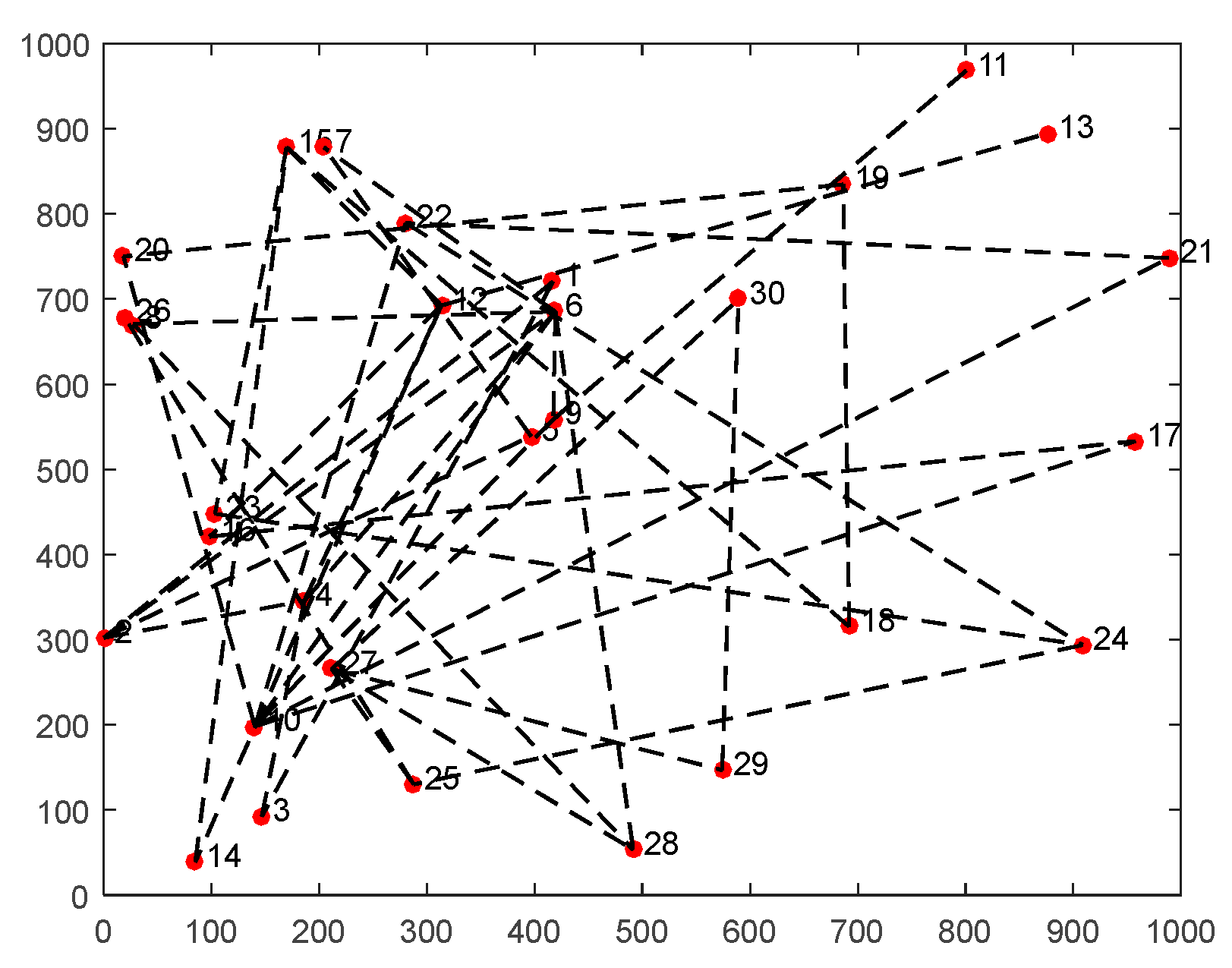
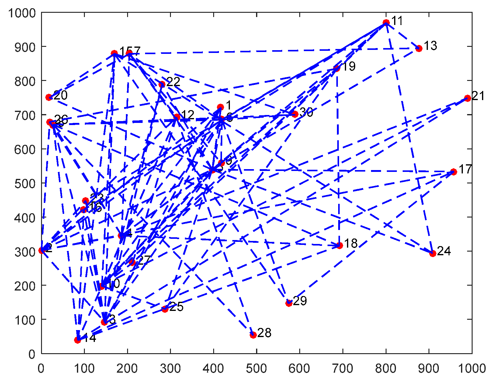
4.1. Initial Topology of Bilateral Subnetwork

The power side builds a topology based on the IEEE30 node system, as shown in Figure 7 below:

The node and line connection relationship of part of the power network is shown in

Table 2. Node and line connection relationship.

Line	From-Node	To-Node
1	1	2
2	1	3
3	2	4
4	3	4
5	2	5
6	2	6
7	4	6
8	5	7

The first column of the table indicates the line serial number, the second column indicates the node at the sending power end of the line, and the third column indicates the node at the receiving power end.

below:

The topology of the cyber side before the failure is shown in Figure 8 below:

The initial number of nodes on the cyber side is 5, and each newly generated node generates 3 edges connected to the old network. As can be seen from the Figure 8, scale-free networks have unequal connectivity between nodes, with large differences between the degrees of each node.

Cyber-side nodes are laid with the power-side nodes, and the information links are denser than those of the transmission lines. Due to the large number of nodes, the adjacency matrix is no longer listed, and only the corresponding connections between the nodes on both sides using the degree-betweenness coupling are shown in

Table 3. Cyber-physical node coupling relationship.

Node of Cyber-Side	Node of Power-Side	Node of Cyber-Side	Node of Power-Side
1	19	16	11
2	28	17	18
3	27	18	17
4	10	19	9
5	6	20	13
6	12	21	14
7	22	22	21
8	2	23	26
9	20	24	29
10	4	25	30
11	15	26	1
12	23	27	5
13	8	28	3
14	24	29	7
15	25	30	16

The numbers listed in Table 3 represent the name or number of the node in their respective subnetworks, such as node 4.

below:

4.2. Establishment of Comprehensive Indexes

As described in Section 2, the active-business importance index is established according to (1) to (5), and then the coupled node pair utilization index is established according to (6) to (11). The horizontal coordinate indicates the information side node number in the coupled node pair. Index weighting coefficients ${\beta }_{cp}$ and ${\gamma }_{cp}$ are taken as 0.5, dual network capacity margin coefficients ${\alpha }_p$ and ${\alpha }_c$ are taken as 0.5, inter-network failure probability $\rho$ is 0.5, load adjustable parameters are selected according to information security partition, I and II are taken as 1.1, III and IV are taken as 1.0.

From Figure 9 and Figure 10, it is seen that there is no linear relationship between the two indexes of vulnerability and importance. From Figure 9, it can be seen that the 6th pair of nodes has the highest active-business degree index, i.e., this pair of nodes is relatively the most important, and from Figure 10, it can be seen that the vulnerability of this pair of nodes is also the highest, so when some nodes on the cyber side are attacked for load reallocation, the load of this pair of nodes should be allocated first, and due to its highest combined vulnerability, it should receive the smallest proportion of the load when accepting the load allocated by the failed neighbor nodes. Then, look at the 1th node pair, which has a low vulnerability and low importance relative to the other nodes, this means even if it is attacked, it should be allocated later, and when its neighbor node fails and needs to allocate load to it, it can take most of the load and thus reduce the burden of other nodes.

4.3. Node Survival Rate under Different Attack Methods

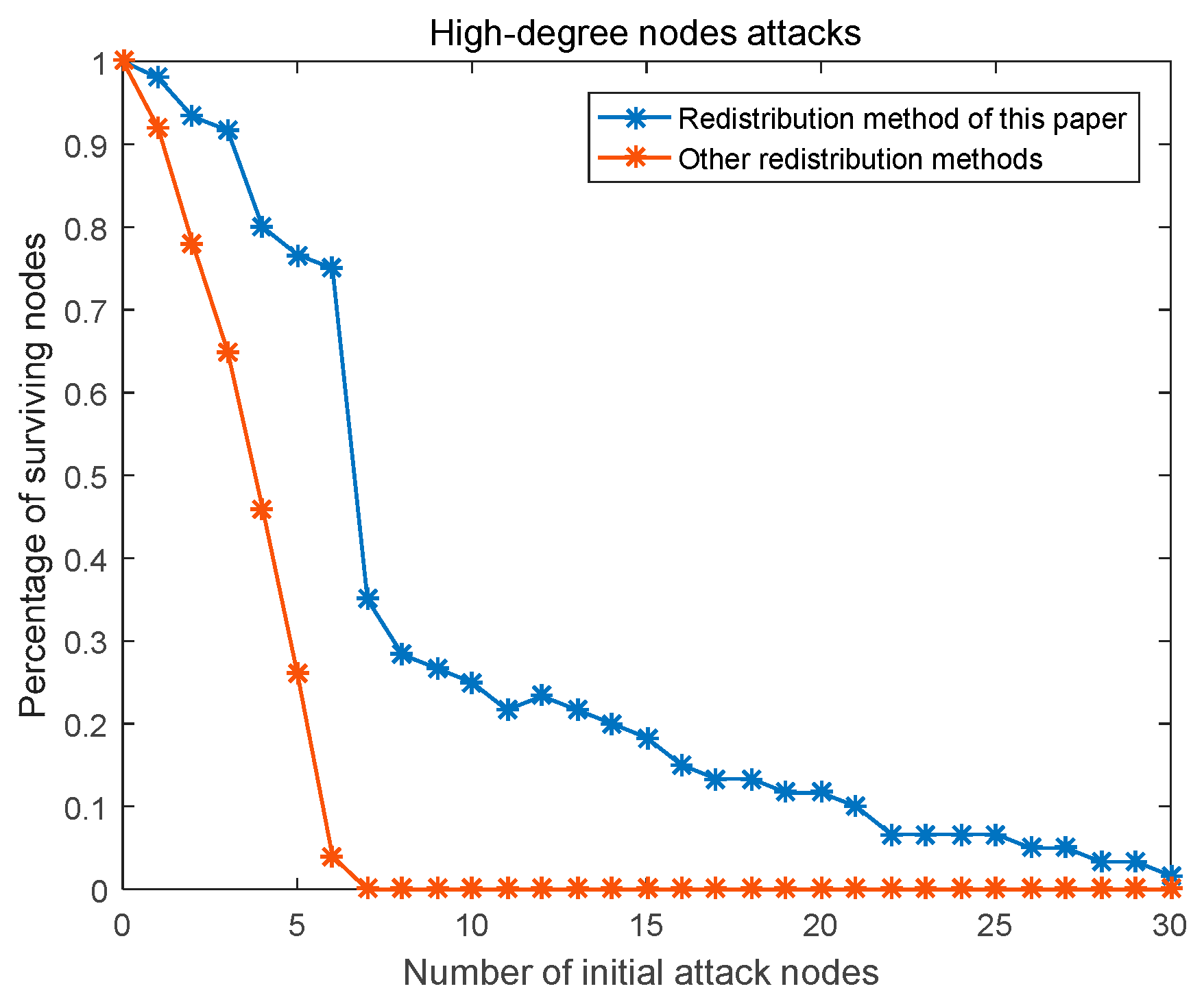
4.3.1. High-Degree Nodes Attacks

The simulation is compared to the existing redistribution methods in the literature, and the number of attacked nodes on the cyber side is increased sequentially by using the high-degree of nodes attack mode.

As can be seen from Figure 11, when the number of attacks is less than 6, the number of remaining nodes under both redistribution methods shows an obvious decreasing trend, and when the number of attacks exceeds 6, the system under the method of this paper still has more than 30% of surviving nodes, while the system under the other methods is close to 0. When the number of attacks is 7, the system under the other methods has completely failed, while the system under the method of this paper still has more than 20% of the survivability of the system, and it only shows a slow decreasing trend as the number of attacks gradually increases.

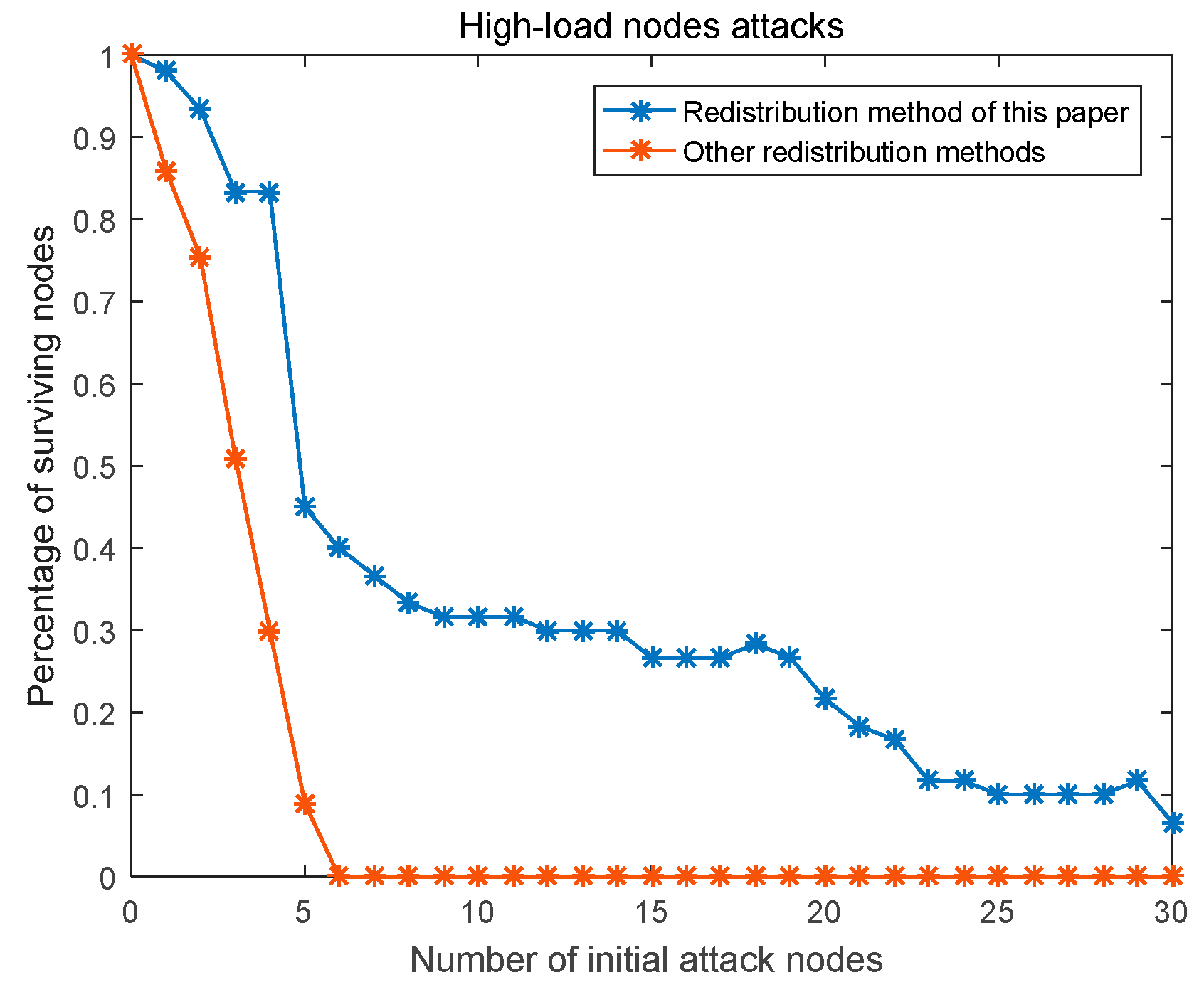
4.3.2. High-Load Nodes Attack

The simulation is compared to the existing redistribution methods in the literature, and the number of attacked nodes on the cyber side is increased sequentially by using the high-load of nodes attack mode.

As can be seen from Figure 12, similar to the degree attack, the blue curve declines more slowly than the red curve in the early stage, and the red curve drops to 0 when the number of attacking nodes is about 6, while the blue curve still has about 40% of the nodes operating normally. In addition, when four nodes on the cyber side suffer from high load attack, the blue curve has an obvious inflection point and the curve drops sharply, which is because the first four nodes on the cyber side with high load carry most of the information flow, and once these four nodes fail, they will cause a large amount of information flow redistribution, which will easily trigger more information nodes to overload and more risk propagation across space to the power side, resulting in the power side being threatened.

4.4. Parameter Analysis

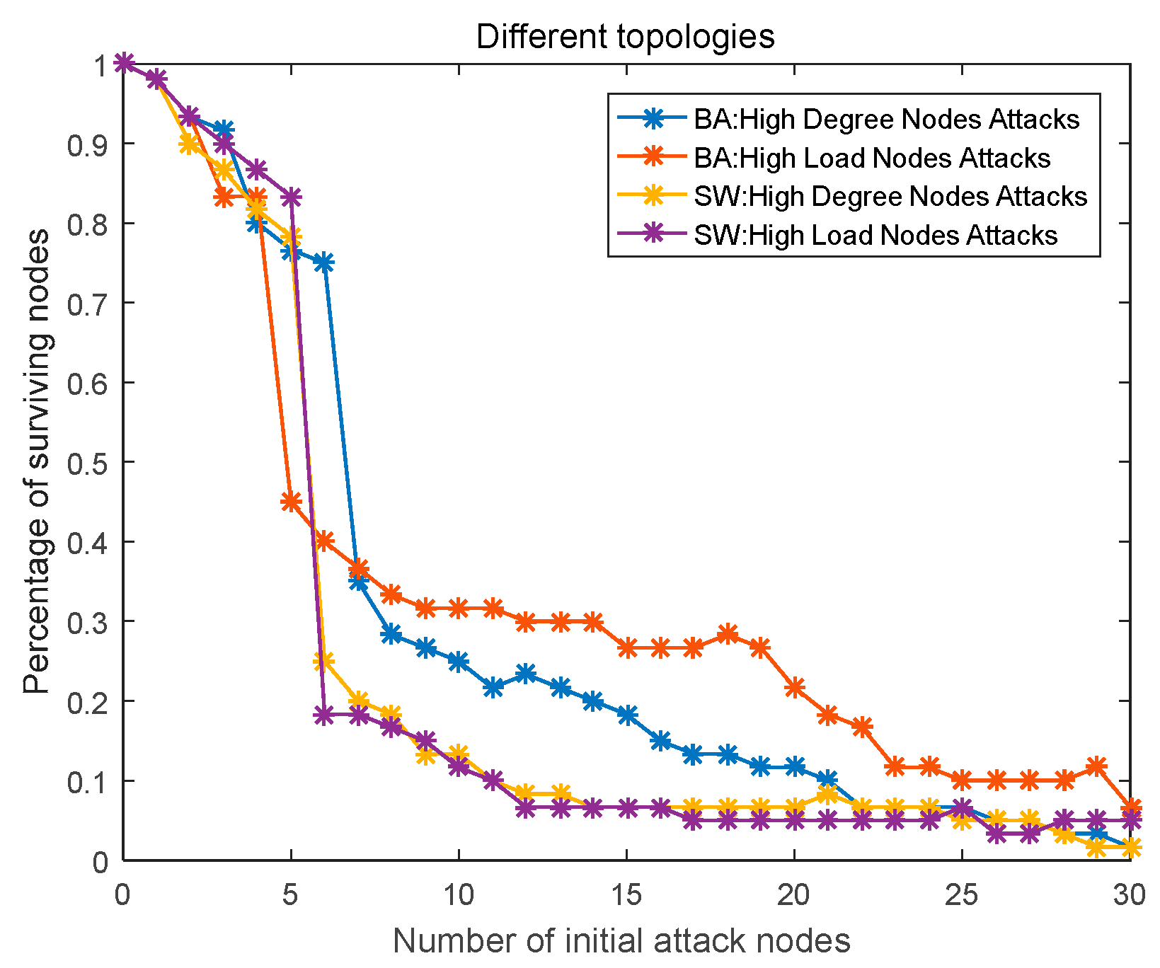
4.4.1. Different Topologies

The cyber-side scale-free network and the small world network are established, respectively. The simulation results of the high-degree node attack and the high-load node attack are performed in these two networks, respectively, as follows in Figure 13.

As can be seen from the Figure 13, the trend of the system survivability curves under both topologies is similar. Under the allocation method in this paper, regardless of whether the scale-free network or the small-world network is used on the cyber side, when the attack ratio is small (less than 6), the loss of the number of nodes in the four curves is comparable, and when the number of nodes in the initial attack is about 6, i.e., the attack ratio is 20%, the curve drop suddenly increases. Besides, when the number of attacks continues to increase gradually, it can be seen that the survivability of the system with the scale-free network is better than that of the small-world network, both under the degree attack and the load attack.

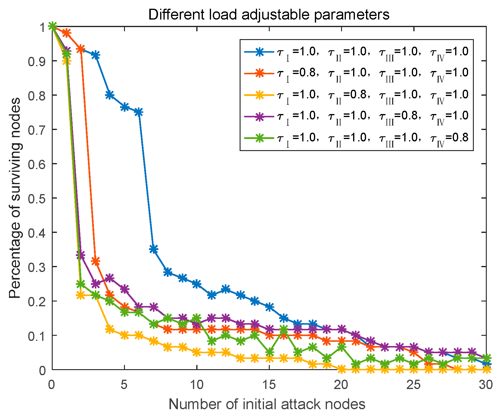
4.4.2. Different Load Adjustable Parameters

The height number attack is used and five groups of load adjustable parameters are taken for comparison, and the results are shown in the following Figure 14.

Where τ_I, τ_I, τ_III, and τ_IV denote the load adjustable parameters of safety zone I, II, and III, IV, respectively.

From Figure 14, it can be seen that there is a decreasing trend of different magnitudes in the five curves. When the load parameters of all security zones are not less than 1, the plunging trend of the curves appears when the number of attack nodes is 6. When the load parameter of zone II is less than 1, the yellow curve in the figure has been at the bottom of several curves, and it can be seen that the overall system survivability is the lowest at this time, which is because the security zone II has a large amount of business and high business importance, and it seems to be the most critical area, so when its load parameter is low, it will lead to a significant decrease in system survivability.

5. Conclusions

In this paper, the topological and functional characteristics of the dual-side network of power CPS are considered, and the active-business degree index and the coupled node pair utilization index, which consider the integrated characteristics of node pairs, are established accordingly. These two indexes are used to deal with the cross-space cascade failure and optimize the load redistribution strategy. The simulation example illustrates that the proposed coupling node pair integrated characteristic index can be effectively used in the load redistribution strategy.