Article

A Quantitative Comparison of Mortality Models with Jumps: Pre- and Post-COVID Insights on Insurance Pricing

1
Department of Accounting, Finance and Actuarial Science, School for Business and Society, University of York, York YO10 5DD, UK
2
Department of Actuarial Sciences, Ankara University, Ankara 06590, Turkey
*
Author to whom correspondence should be addressed.
These authors contributed equally to this work.
Risks 2024, 12(3), 53; https://doi.org/10.3390/risks12030053
Submission received: 26 January 2024 / Revised: 29 February 2024 / Accepted: 10 March 2024 / Published: 14 March 2024
(This article belongs to the Special Issue Extreme Events: Mortality Modelling and Insurance)

Abstract

:
Population events such as natural disasters, pandemics, extreme weather, and wars might cause jumps that have an immediate impact on mortality rates. The recent COVID-19 pandemic has demonstrated that these events should not be treated as nonrepetitive exogenous interventions. Therefore, mortality models incorporating jump effects are particularly important to capture the adverse mortality shocks. The mortality models with jumps, which we consider in this study, differ in terms of the duration of the jumps–transitory or permanent–the frequency of the jumps, and the size of the jumps. To illustrate the effect of the jumps, we also consider benchmark mortality models without jump effects, such as the Lee-Carter model, Renshaw and Haberman model and Cairns-Blake-Dowd model. We discuss the performance of all the models by analysing their ability to capture the mortality deterioration caused by COVID-19. We use data from different countries to simulate the mortality rates for the pandemic and post-pandemic years and examine their accuracy in forecasting the mortality jumps due to the pandemic. Moreover, we also examine the jump-free and jump models in terms of their impact on insurance pricing, specifically term annuity and life insurance present values calibrated for both pre- and post-COVID data.

1. Introduction

In an aging world, the accurate modelling of human mortality becomes crucial due to demographic transitions, catastrophic events, healthcare advancements, and societal shifts. Mortality models examine the factors influencing life expectancy, enabling pension plans, insurers, and actuaries to make informed decisions regarding healthcare planning, pension systems, and societal well-being. Since the early 1990s, researchers have developed numerous stochastic models to capture and quantify the patterns of human mortality over time. These models include the Lee–Carter model, its extensions and alternatives (Brouhns et al. 2002; Lee and Carter 1992; Renshaw and Haberman 2006), the P-splines model (Currie et al. 2004), and the Cairns–Blake–Dowd model (Cairns et al. 2006, 2007).
However, recent decades have witnessed significant changes in mortality rates in many countries. Generally, there has been an improving trend, but for some, the last 10 to 20 years have seen either a slowdown or even a reversal of some of these improvements, further disrupted by the COVID pandemic (Cairns 2023). Catastrophic events, such as COVID-19, are referred to as mortality risks, and they may cause sudden increases in mortality rates over certain periods of time, while these events are infrequent, their occurrences could lead to numerous death claims and mortality jumps on the mortality curve.
Particularly, COVID-19 has highlighted the crucial consequences of these catastrophic events and emphasised the importance of preparing for future outbreaks. Hence, it is essential to incorporate mortality jumps in the modelling process. Although many mortality models without jump effects exist, only a few have been developed that consider mortality jump effects with a focus on the time series properties of mortality. These include Chen and Cox (2009), Cox et al. (2006), Deng et al. (2012), and Özen and Şahin (2020), which differ in terms of the duration of the jumps–transitory or permanent–frequency of the jumps, and size of the jumps.
To provide a comprehensive overview, Regis and Jevtic (2022) also present a review of single and multi-population continuous time mortality models with and without jumps. Specifically, they focus on multi-population mortality models with jumps since these models are needed to describe the heterogeneous impact of mortality shocks across cohorts of individuals. An example of a discrete time two-population model with jump effects can be found in Özen and Şahin (2021).
Acknowledging the dynamic nature of global mortality trends and the significant impact of events like the COVID-19 pandemic, this study aims to assess the efficacy of mortality models. We aim to compare and discuss the performance of mortality models, both with and without jump effects, analysing their ability to capture the mortality deterioration caused by COVID-19. The mortality models without jump effects include the Lee–Carter model, Renshaw and Haberman model, and Cairns–Blake–Dowd model. In contrast, the Lee–Carter model with permanent jump effects, transitory jump effects, exponential transitory jumps, and renewal process effects are employed as the mortality models with jump effects. We utilise mortality data from various countries obtained from the Human Mortality Database (2023) (HMD). Given that COVID-19 is a potential cause for a jump in the mortality curve, our primary objective is to identify the mortality models that can accurately forecast COVID deaths from 2020 onward. To achieve this, we initially fit the models to the pre-COVID data and forecasted the pandemic and post-pandemic years. We compared the performance of the models considering both in-sample and out-of-sample forecasting, analysed the estimated parameters, and focused specifically on the time-dependent parameter in which the explicit jumps were added for the mortality jump models discussed.
Furthermore, we present the valuation of mortality-related insurance products, such as term life annuity and life insurance, using both the jump-free and jump models calibrated for pre- and post-COVID data.
The remainder of this paper is structured as follows: Section 2 describes the mortality models utilised in this study. Section 3 presents the results and compares the models in terms of model parameters, model fits, in-sample, and out-of-sample forecasts. Section 4 provides the impact of the pre- and post-COVID calibration of the jump-free and jump models on the valuation of mortality-related insurance products. Finally, Section 5 introduces new directions of research and concludes the paper.

2. Mortality Models

This section introduces the mortality models considered in this study. To provide a comprehensive analysis of mortality jump models and their performance in forecasting COVID-19 deaths, we compare them with the Lee and Carter (1992) (LC) model with random walk, which serves as the benchmark model. Additionally, we include the Renshaw and Haberman (2003) (RH) model as a representative of age-period-cohort (APC) models and the Cairns et al. (2006) (CBD) model as the two-factor mortality model.

2.1. The Lee–Carter Model

The Lee–Carter model describes the logarithm of central death rates as follows:
ln ( m x , t ) = α x + β x κ t
Here, α x represents the average of ln m x , t over time t, κ t captures the long-term improvements of mortality, and b x measures the age sensitivity of mortality as κ t changes. The model parameters are estimated using a two-stage singular value decomposition. To ensure a unique solution for the parameters, the estimation method requires the following identifiability constraints:
x β x = 1 and t κ t = 0 .
The estimation process involves two stages. Firstly, the singular value decomposition method is applied to the ln ( m x , t ) α x matrix to obtain the estimates of β x and κ t . In the second stage, given the α x and β x , the κ t parameters are re-estimated. This step ensures equality between the actual sum of deaths at time t and the implied sum of deaths at time t.
D t = x ( P x , t exp ( α x + β x κ t ) )
where D t gives the actual sum of deaths at time t, and P x , t is the population in age group x at time t.
In this paper, following Brouhns et al. (2002) and using the StMoMo R Package (Villegas et al. 2018), we employ the MLE method to estimate the parameters. We fit the Lee–Carter model assuming a Poisson distribution of the number of deaths, using the log link function to target the force of mortality μ x , t . Hence, the predictor η x , t is given by the following:
η x , t = α x + β x κ t
We adopted the notation from Villegas et al. (2018). In the original Lee–Carter model, the κ t parameters are modelled using a random walk with drift, as in Equation (2):
κ t + 1 = κ t + μ + σ Z t + 1
where Z t + 1 has a standard normal distribution.
The Lee–Carter model with a random walk κ t is considered as a benchmark model in this paper.

2.2. Renshaw and Haberman Model

As a second model, we use the age-period-cohort model proposed by Renshaw and Haberman (2003), which is an extension of the Lee–Carter model.
η x , t = α x + β x κ t + γ t x
Here, γ t x represents the cohort effect. Mortality projections for this model are obtained by forecasting the time series of the estimated κ t and γ t x as univariate ARIMA processes under the assumption of independence between the period and cohort effects.

2.3. Cairns–Blake–Dowd Model

Cairns et al. (2006) proposed a mortality model with two age-period terms with pre-specified age-modulating parameters β x ( 1 ) = 1 and β x ( 2 ) = x x ¯ , no cohort effect, and no static age function. The CBD model is given as follows:
η x , t = κ t ( 1 ) + ( x x ¯ ) κ t ( 2 ) ,
where x ¯ is the average age in the data. The period effects κ t ( 1 ) and κ t ( 2 ) are modelled by using a bivariate random walk with drift to obtain mortality forecasts (Villegas et al. 2018).

2.4. Jump Effect Models as Extensions to the Lee–Carter Model

While the Lee–Carter model is inherently designed for long-term mortality analysis, its time-varying mortality index must incorporate short-term effects to enhance the efficacy of mortality modelling. This necessity has led to the introduction of jump effect models.
In this section, we will present one permanent jump model and two transitory jump models. These models are regarded as extensions of the Lee–Carter model, as they specifically address the time-varying parameter κ t and incorporate explicit jump effects.
Although our study primarily focuses on jump extensions of the Lee–Carter model, it is important to note the recent literature on extensions of the CBD and RH (APC) models to include jumps. Venter (2022) proposes an ’event jump model’ as an extension to the RH model, introducing a proportional jump to mortality rates that varies by year and represents a constant percentage increase across ages and cohorts. In this model, higher-mortality groups experience the most significant increases in the number of deaths, although all groups are affected. Each year is assigned a jump factor, but these may be negligibly small for normal years. The paper fits mortality curves across age, cohort, and time parameters using regularized smoothing splines, with fit quality assessed using cross-validation criteria. In two more recent papers, Richards (2023) and Schnürch et al. (2022), the APC and CBD model have been adapted to include COVID jumps along with the others. Richards (2023) focuses on the robustification of forecasts for different types of mortality models, including the CBD model. They identify outliers in the residuals, co-estimate outlier effects with other parameters to remove bias and distortion from the forecasts caused by mortality shocks, providing a robust starting point for projections. On the other hand, Schnürch et al. (2022) induce a log-parallel shift to the CBD model, calibrate the time-dependent parameters by linear regression, and obtain forecasts via a two-dimensional random walk with drift for five-group age ranges starting at 60.

2.4.1. κ t with Permanent Jump Effect

Cox et al. (2006) proposed a mortality model with permanent jump effects, combining geometric Brownian motion and a compound Poisson process. However, we consider the model in a discrete-time setting, following Chen and Cox (2009), for the consistency of model comparisons.
Therefore, let N t denote the number of jumps occurring in year t. For simplicity, it is assumed that there is at most one jump event in each year, with the probability of a jump being p; that is, as follows:
N = 1 , with probability p , 0 , with probability 1 p .
The jump severity variable, Y, is identically and independently distributed normal variables with mean m and standard deviation s. Moreover, Y and N are independent.
As in Chen and Cox (2009), the evolution of the mortality index κ t with permanent jump effects can be written as follows:
κ t + 1 = κ t + μ p m + σ Z t + 1 , if N t + 1 = 0 , κ t + μ p m + σ Z t + 1 + Y t + 1 , if N t + 1 = 1 ,
where μ and σ are constants, and Z t is a standard normal random variable that is independent of Y and N.

2.4.2. κ t with Transitory Jump Effect

In the permanent jump model, if a jump event occurs in year t + 1 , the size of the jump Y t + 1 is incorporated into the mortality factor κ t + 1 , and this jump effect persists indefinitely. However, many of these jumps are attributed to short-term catastrophic events, resulting in a transient impact on the mortality curve. Therefore, mortality models with transitory jump effects are deemed more suitable for modelling extreme mortality risks.
We consider the transitory jump effects as proposed by Chen and Cox (2009). In their model, the mortality factor is modelled as follows:
κ ˜ t + 1 = κ ˜ t + μ + σ Z t + 1 κ t + 1 = κ ˜ t + 1 + Y t + 1 N t + 1
where κ ˜ t denotes the jump-free mortality factor, and κ t is the actual mortality factor including jumps.
Equation (6) indicates that extreme mortality events only have an impact on κ t + 1 , not on κ ˜ t + 1 . Therefore, if a mortality jump occurs in a given year, it will revert to the normal mortality level shortly thereafter.

2.4.3. κ t with Exponential Transitory Jumps and Renewal Process Effect

The model with exponential jumps and a renewal process is proposed by Özen and Şahin (2020). The originality of the model lies in employing the renewal process instead of the Poisson process. In the Poisson process, waiting times between mortality jumps are constant, meaning that the occurrence of previous catastrophic events has no impact on the likelihood of the next event. To incorporate the history of events, one approach is to consider the renewal process, featuring a time-varying hazard function reflecting the waiting times between catastrophic events. An increasing hazard function indicates longer waiting times between events than a decreasing hazard function. In these models, waiting times between catastrophic events are no longer constant; however, the occurrence of at least one event (versus none) up to time t influences the probability of another event’s arrival in t + Δ t by the time-varying hazard function. Hence, by employing the renewal process, we aim to integrate the history of catastrophic events into the mortality modelling process.
In the proposed model, the mortality factor is modelled as follows:
κ t = κ 0 + μ 1 2 σ 2 δ θ t + σ Z t + i = 1 N t Y i
where Z t is standard Brownian motion, and N t is a renewal process with parameters α and β . The expected value of the process would give the expected frequency of the jumps. Here, Y i denotes a sequence of independent and identically distributed exponential random variables representing the size of the jumps with parameter η . The terms δ and θ denote the expected value of the jump size and the jump frequency, respectively.
In the renewal process, to calculate jump probabilities, we need to specify the distribution of the inter-arrival times between mortality jumps. Therefore, we must first detect the mortality jumps on the mortality curve. This is achieved by employing the method proposed by Chen and Liu (1993) to identify outliers in the mortality index. The outlier detection approach classifies the outliers into four categories based on their impacts on the time series. In this study, we focus on the additive outliers since they have one short and immediate effect on the time series (Chen and Cox 2009). After performing the outlier detection process and obtaining the additive outliers on the mortality curve, as in Li and Chan (2005), we consider the events as outliers that are greater than the critical value of C = 2.5 . Thereafter, we need to specify the inter-arrival times between these events. The years of detected outliers and their test statistics are shown in Table 1. Subsequently, we determine the distributions of the inter-arrival times of jumps to make predictions for future expected frequencies of outliers (for model details, refer to Özen and Şahin 2020).
However, this process requires a decent sample size for distribution fitting. The detected outliers are given in Table 1, showing seven outliers for Spain, Sweden, and Switzerland, five for Denmark, three for the UK, and two for Japan. This indicates that the size of the data to fit a distribution for inter-arrival times is six for three countries in the best case. It is still too few to fit a distribution properly.
The literature on the distribution of the inter arrival times suggests lognormal, Weibull, and gamma distributions (McShane et al. 2008). Due to the small number of jumps and hence inter-arrival times, we consider the distributions proposed by the existing literature and compare the log-likelihoods and BICs of the overall model for each distribution. Then, we choose the distribution for the inter-arrival times that provides the best fit for each country. Therefore, the analysis reveals that the distributions of inter-arrival times are lognormal for Denmark and Switzerland and Weibull for Japan, Spain, Sweden, and the UK.
Based on the specified distribution, convolution methods are used to obtain the jump frequencies in the renewal process. Let P ( n ) be the probability of n jumps occurring in the given time. Moreover, F ( t ) and f ( t ) are the distribution and density functions of the inter-arrival times between jumps. Then, the jump probabilities are obtained by P ( 0 ) = 1 F ( t ) and P ( n ) = 0 t P n 1 ( t s ) f ( s ) d s (for more details, see Özen and Şahin 2020).
Table 1 presents the years of the detected outliers for Denmark, Japan, Spain, Sweden, Switzerland, and the UK after fitting time series models to the obtained κ t values using the Lee–Carter model. It is crucial to note that the detected years are subject to change due to the fitted time series model. We selected the best-fitting models, which are outlined in the table. The provided years for outliers, hence, mortality jump years, are determined based on the residuals from the given time series models. Notably, for Japan, those two jumps coincide with the Fukui earthquake (1948) and Isahaya flood (1957); for Spain, we observed seven jumps—1918–1919 represents the Spanish flu, and 1942 represents the Civil War. Likewise, for Sweden and Switzerland, we observed seven jumps—1918–1919 represents the Spanish flu. In the case of the UK, three jumps are observed, with 1944 representing World War II. Table 1 also presents the mean absolute percentage errors (MAPE) for each country. As demonstrated in the next section, κ t over time for Japan during the fitted period is notably smooth compared to the other countries, suggesting minimal indications of jumps in the mortality index.
In Table A1, we utilised all available up-to-date data for six countries to observe and compare the number of jumps and jump years in pre- and post-COVID periods. For Spain, Sweden, Switzerland, and the UK, the COVID pandemic caused statistically significant jumps based on the outlier analysis discussed above. The inclusion of the COVID years either increased the number of observed jumps or changed the observed jump years while keeping the number of jumps the same for the time index parameter.

3. Results and Discussion

This section presents results from different models for each country to compare and discuss their fits to the historical data and the performance of the models for forecasting COVID-19 deaths from 2020 onward.

3.1. Model Comparisons

3.1.1. Parameter Estimation Process
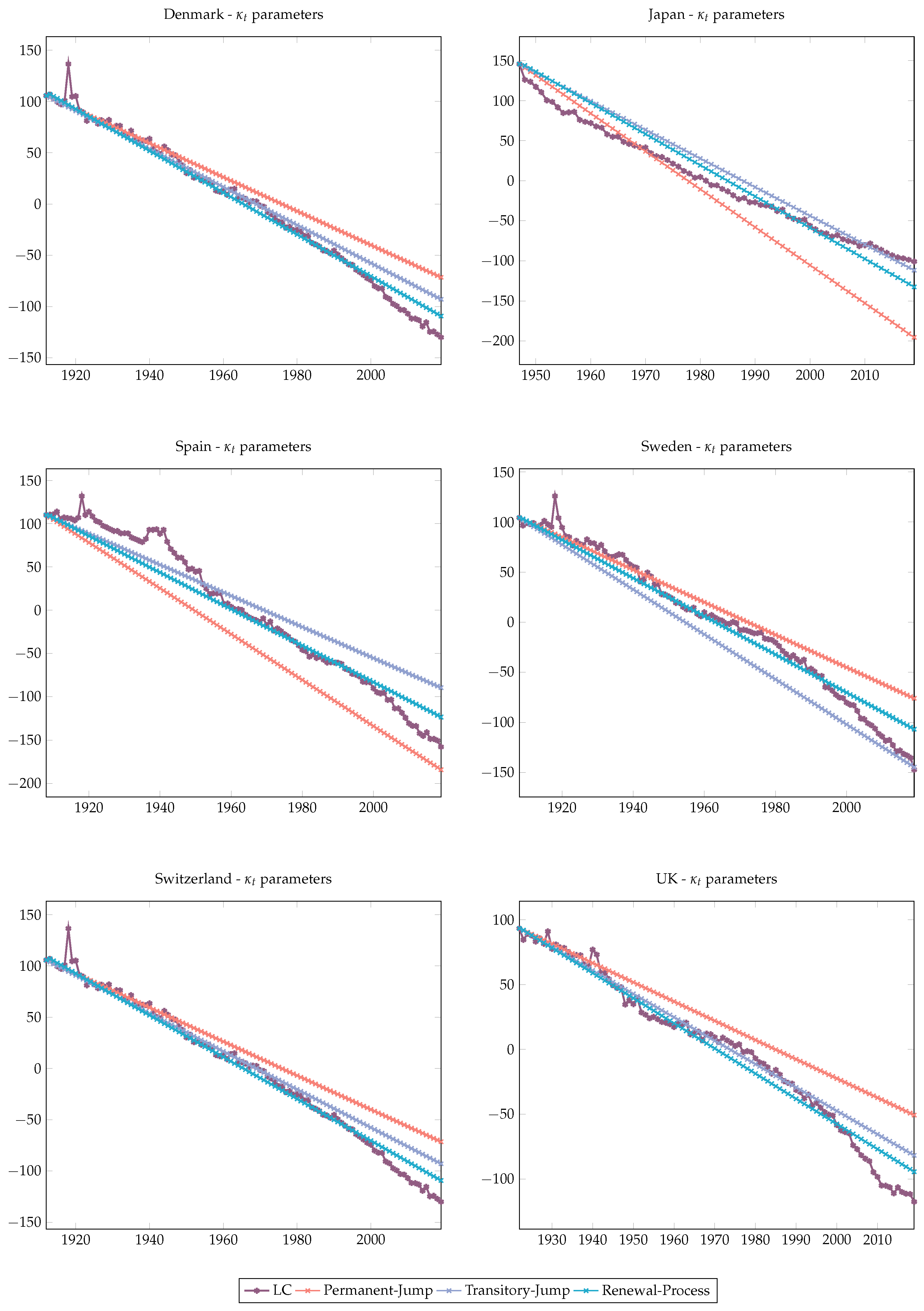
It is useful to provide an explanation of the estimation process using the jump models considered in this study. As described in Chen and Cox (2009) and Özen and Şahin (2020), the estimation procedure involves multiple stages. First, the Lee–Carter model is fitted to the data by assuming a Poisson distribution for total death counts in year t. Using the maximum likelihood method, we estimate the parameters for the Lee–Carter model. We used the R StMoMo package (Villegas et al. 2018) with a log link function to estimate the Lee–Carter parameters. Once κ t is estimated, we take the values as a time series and fit the jump processes introduced in three different jump models. For the discretised permanent jump and the transitory jump models, the parameters associated with the jump effects and the random walk with drift are estimated using the method of conditional maximum likelihood. For the transitory jump model with a renewal process and exponential jumps, we used specified distributions for inter-arrival times and then applied the convolution method to obtain the jump frequencies in the renewal process using the conditional maximum likelihood method. We do not re-estimate α x and β x in any of these processes after the κ t is modelled using jump processes. The original Lee–Carter α x and β x estimates have been used for all forecasts and diagnostic checks throughout.
Moreover, in none of these jump models has the age pattern of mortality jumps been considered. Jumps vary by time and are the same for all ages, which may not be realistic for some catastrophic events. However, the multiple-stage estimation process described above is convenient and less complicated under these circumstances. On the other hand, as discussed in Liu and Li (2015), all relevant parameters can be estimated in a single estimation algorithm, as suggested by Haberman and Renshaw (2012) in Route II methodology. Considering the structures of the jump models discussed above, this approach is beyond the scope of this paper.

3.1.2. Fitted κ t Parameters

Firstly, we present the κ t parameters obtained from the fitted LC model for each country and proceed to compare these estimates with those derived from the following three distinct jump models: κ t with a permanent jump, κ t with a transitory jump, and κ t with a renewal process.
Figure 1 visually represents the comparison, highlighting that the κ t parameters obtained from the transitory jump models exhibit a closer alignment with the original LC parameters across all examined countries. This observation is also supported by the MAPE values presented in Table 2.
The utilisation of jump models is particularly insightful, as they contribute to the production of smoother κ t trajectories by explicitly incorporating jumps in the mortality time index. A smoother trajectory that closely mirrors the LC parameter is indicative of a superior fit.
As demonstrated in Figure 1, the permanent jump model consistently and notably underestimates the time-dependent parameters in Spain, while frequently overestimating κ t for Denmark, Sweden, Switzerland, and the UK in comparison to the LC parameter. In contrast, both transitory jump models yield more accurate fits. The renewal process utilising the exponential jump model is particularly noteworthy, as it generates trajectories that closely correspond to the LC parameter across all six countries.
It is crucial to acknowledge that, in the case of Japan, the limited number of jumps during the considered period complicates the applicability of any of the jump models. Consequently, none of the models appear to be ideal for this specific scenario. This observation highlights the intricate challenges inherent in mortality jump modelling, especially in situations where jump occurrences are sparse and jump sizes are relatively small.

3.1.3. Bayes Information Criterion

The Bayes information criterion (BIC) serves as a means to compare models and discern which one better fits the data. A key aspect of BIC is its ability to compare models that are not necessarily nested.
The BIC for mortality models is defined as follows:
BIC = l ( ϕ ^ ) 1 2 υ log N
Here, ϕ denotes the parameter vector, and ϕ ^ stands for its maximum likelihood estimate. In this context, l ( ϕ ^ ) represents the maximum likelihood, N is the number of observations, and υ is the number of parameters estimated from the mortality models (Cairns et al. 2007).
To determine which jump effect better fits the mortality data, we initiate the comparison by examining the mortality time indices (for estimated κ t s), parameter estimations, and BIC values obtained for those κ t s in Table 3. Subsequently, we extend our comparison to encompass all jump-free and jump models, evaluating their overall BIC values (not limited to κ t s alone) as presented in Table 4. It is noteworthy that a higher BIC value indicates a better fit.
Table 3 presents a comparative analysis between the Lee–Carter with random walk (LC-RW) model and three jump models, all fitted to the κ t parameters derived from the benchmark LC model and its derivatives. Among these models, the two transitory jump models exhibit superior fits, as evidenced by their lower BIC values, in contrast to both the LC-RW (except Japan for one of the models) and permanent jump model. It is essential to note that while the differences in BIC values may seem substantial, a more dependable basis for comparing the performance of the models is provided by the mean absolute percentage errors (MAPE), which is discussed in the following subsection. In Table A2, we utilised all available up-to-date data for six countries to observe changes in model parameters and in-sample fits for pre- and post-COVID periods. The results indicate that although including COVID data changed the parameters, the performance of the models did not change significantly.
On the other hand, Table 4 offers a more detailed comparison among three jump-free models, namely, LC-RW, RH, and CBD, and three jump models derived from the LC model. This comparison is facilitated by presenting the overall model BICs and MAPEs. Given the diverse structures of the models, the BIC values appear quite distinct. However, it is evident that, in general, and particularly with transitory jump models, the jump models consistently outperform the benchmark jump-free models.

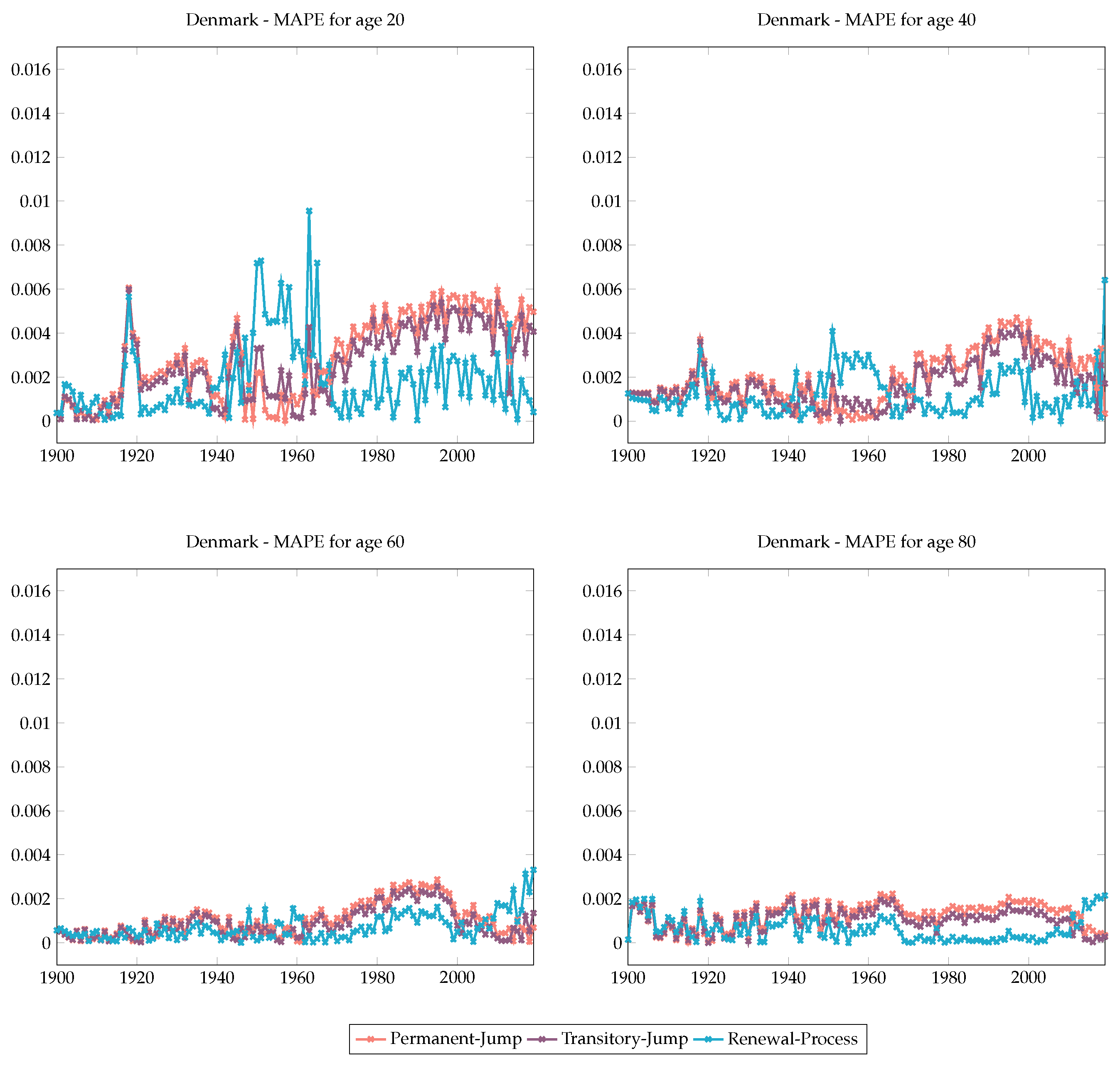
3.1.4. Mean Absolute Percentage Error (MAPE)

The mean absolute percentage error (MAPE) stands out as a widely used metric for assessing prediction accuracy in mortality modelling. Its formulation is given by the following:
M A P E i = 1 N i x , t m ^ x , i , t m x , i , t m x , i , t
In this equation, N i represents the number of observations in each population, calculated as the product of the number of ages and the number of years. Here, m ^ x , i , t denotes the estimated number of deaths, while m x , i , t represents the observed number of deaths for a specific time (t), age (x), and population (i).
We employ MAPE to assess the in-sample prediction performance of the models. Initially, we consider all ages in Table 4 as model MAPEs. Subsequently, we present graphs for specific ages (20, 40, 60, and 80) to observe age-specific variations, focusing exclusively on jump models for different countries in Figure A1, Figure A2, Figure A3, Figure A4, Figure A5 and Figure A6 in Appendix C. These graphs share a common y-scale, facilitating the comparison of different models and their effectiveness in capturing mortality deterioration across various countries.
Contrary to the BIC values, the overall MAPE values in Table 4 present a much closer scale when comparing jump-free and jump models. However, the RH model stands out by producing relatively distinct and higher MAPEs compared to the others. Consistently lower MAPEs obtained from the jump models indicate better fits for the listed countries, with transitory jump models—particularly the renewal process model—exhibiting superior fits.
Furthermore, the MAPE results illustrated in Figure A1, Figure A2, Figure A3, Figure A4, Figure A5 and Figure A6 in Appendix C indicate that better fits, characterised by lower MAPE values and reduced volatilities, are observed as ages increase for almost all countries and all three models. Notable differences emerge between the models, with the two transitory jump models consistently demonstrating superior fits and yielding the lowest MAPE values across all countries and ages, except for Japan.
The model incorporating an exponential jump with the renewal process consistently provides the lowest MAPE for all countries and ages, with the same exception, Japan, despite the volatilities observed in the graphs. Additionally, for Japan, the LC-RW model exhibits a slightly better fit as age advances, a detail not clearly depicted in the graphs. This observation aligns with the κ t parameter graphs in the preceding section for Japan, where the time series graph appears notably smoother, suggesting fewer significant jumps compared to other countries discussed in this paper. Essentially, this implies that when there are no jumps or jumps with relatively small magnitudes, regardless of their frequency, jump-free models tend to outperform models with jumps.

3.1.5. Forecasts

Table 5, Table 6, Table 7, Table 8, Table 9 and Table 10 present forecasts for the COVID and post-COVID years, including quantiles and ranges derived from 100,000 simulations for the number of deaths for age 75, serving as an example for six countries. The models, encompassing both jump-free and explicit jump models, were fitted up to 2019, the last pre-COVID year, and are compared in forecasting the number of deaths for the COVID and post-COVID years based on data availability from the HMD website. The forecast quantiles, represented by colours, indicate the intervals within which the observed number of deaths fall. The final columns of the tables present the forecast ranges, with bold ones indicating the smallest range for that specific year.
In Table 5, only the CBD model forecasts COVID deaths for all three years from 2020 to 2022 for Denmark, with much higher uncertainty as indicated by the ranges, which are from four to six times larger compared to the other models. The LC-RW model captures the number of deaths for 2020 in the first quantile, along with the CBD and all three jump models, while the RH provides true forecasts for deaths at age 75 in the third quantile. Comparing to the observed values in Denmark, the jump models accurately forecast the number of deaths for 2020 and 2022 with relatively small uncertainty given as the range in the final column. The permanent jump model provides the most accurate forecasts.
For Japan, in Table 6, all six models provide forecasts with varying degrees of uncertainty. Permanent jump and transitory jump models offer smaller forecast intervals compared to the other models whilst the RH model only forecast 2020 correctly with the highest certainty. The transitory jump model with the renewal process presents a less accurate fit, consistent with its structure, which requires the distribution of the inter-arrival times, a challenge when only two observations are available. It is important to note that the number of deaths in 2019 for age 75 is higher than the COVID and post-COVID years, and thus death rates. The CBD model provides the second largest ranges after the renewal process model.
In Table 7, only RH and CBD models capture the high jump in the first COVID year (2020) in Spain, however, with greater uncertainty. All jump models, but particularly the transitory jump model, present much narrower ranges, which also prevents them from capturing the significant jump in Spain.
For Sweden, in Table 8, except for the RH model, which only forecasts 2022 correctly, all other models forecast COVID deaths within the provided ranges for at least the first two years (2020 and 2021). Particularly, the transitory jump models offered more accurate forecasts with smaller ranges.
Table 9 shows that the transitory jump model with renewal process forecast the number of deaths for all years by providing the smallest forecast ranges for Switzerland.
In the UK (Table 10), there is a notable jump in the number of deaths due to COVID compared to 2019, and two transitory jump models provide the correct death rates with more accuracy compared to the LC-RW and the CBD models, which also included the true forecasts in their ranges. Moreover, the RH model did not forecast the death rates correctly in the provided forecast ranges.
Those results do not change significantly for other ages, such as age 60, while all six models perform differently for different countries, jump models outperform the jump-free models in forecasting COVID deaths by providing more accurate forecasts in 60% of the cases. Upon examining the RH model, which has provided the most accurate forecast for the remaining 33%, we could draw a conclusion about the shortcomings of the jump models under consideration as missing age/cohort-specific jump effects. One common feature of the jump models discussed in this paper is that those models assume that the distribution of the jump effects and general mortality improvements across ages are identical. However, this assumption is not supported by the historical data as explained below, considering the heterogeneous effect of catastrophic events on the mortality curve. In order to address this limitation, Liu and Li (2015) introduced two transitory jump models, which capture the age pattern of mortality jumps by extending the transitory jump model proposed by Chen and Cox (2009). Their study also showed that the age pattern of mortality jumps has a significant impact on the estimated CAT bond prices. Whilst this extension can be considered for the transitory jump model with a renewal process, it is not straightforward due to the differing structure of the κ t jump process compared to the process proposed by Chen and Cox (2009). This will be discussed further in conclusion section as a future study direction.
The mortality jump models employed in this paper were proposed to be calibrated using a long observation period of mortality data (see, for example, Chen and Cox 2009; Özen and Şahin 2020). On the one hand, this approach makes sense because it enables the incorporation of several extreme events and their effects on mortality rates for different age groups. For instance, while the Spanish flu disproportionately affected younger ages, COVID-19 has had a more significant impact on older age groups. Additionally, wars might influence the mortality rates of younger and middle-aged individuals, as well as males more than females, while heatwaves might affect a wider age group and all genders. Considering all these heterogeneous effects of extreme events on mortality curves, it seems more reasonable to calibrate the jump models using data that includes all possible ages or age groups, as well as a longer historical dataset.
On the other hand, the parameters of the models, which are assumed to be constant over time and given in Table 3, are estimated based on a time invariance assumption. However, this assumption has been proven to be incorrect for many populations over long calibration periods in the literature (see Schnürch et al. 2023 for more details). This distortion in the time variance assumption, which encompasses different mortality regimes over time, might have been reflected in the forecast performance of the jump models in pandemic years. A reduced calibration data period could be employed to ensure the stability of the model parameters, which is also the case for jump-free models.

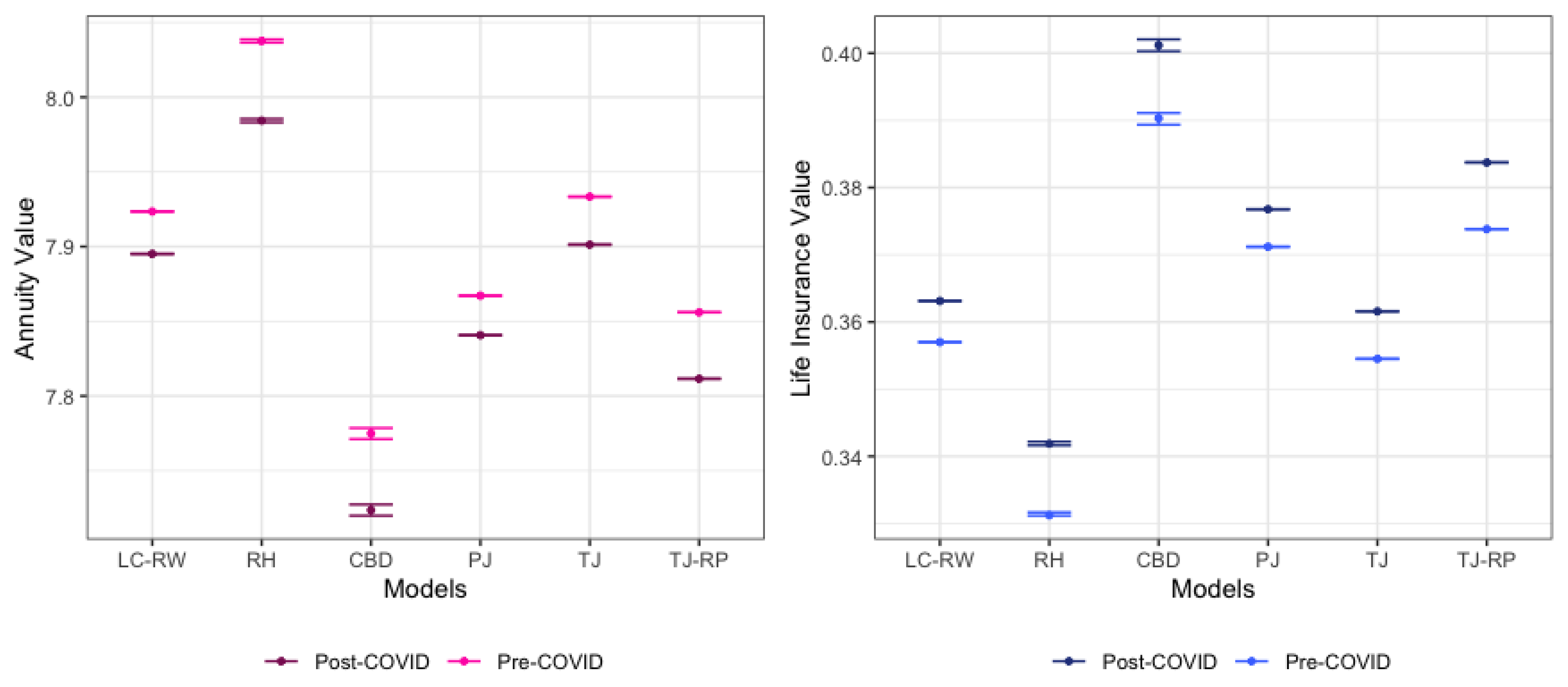
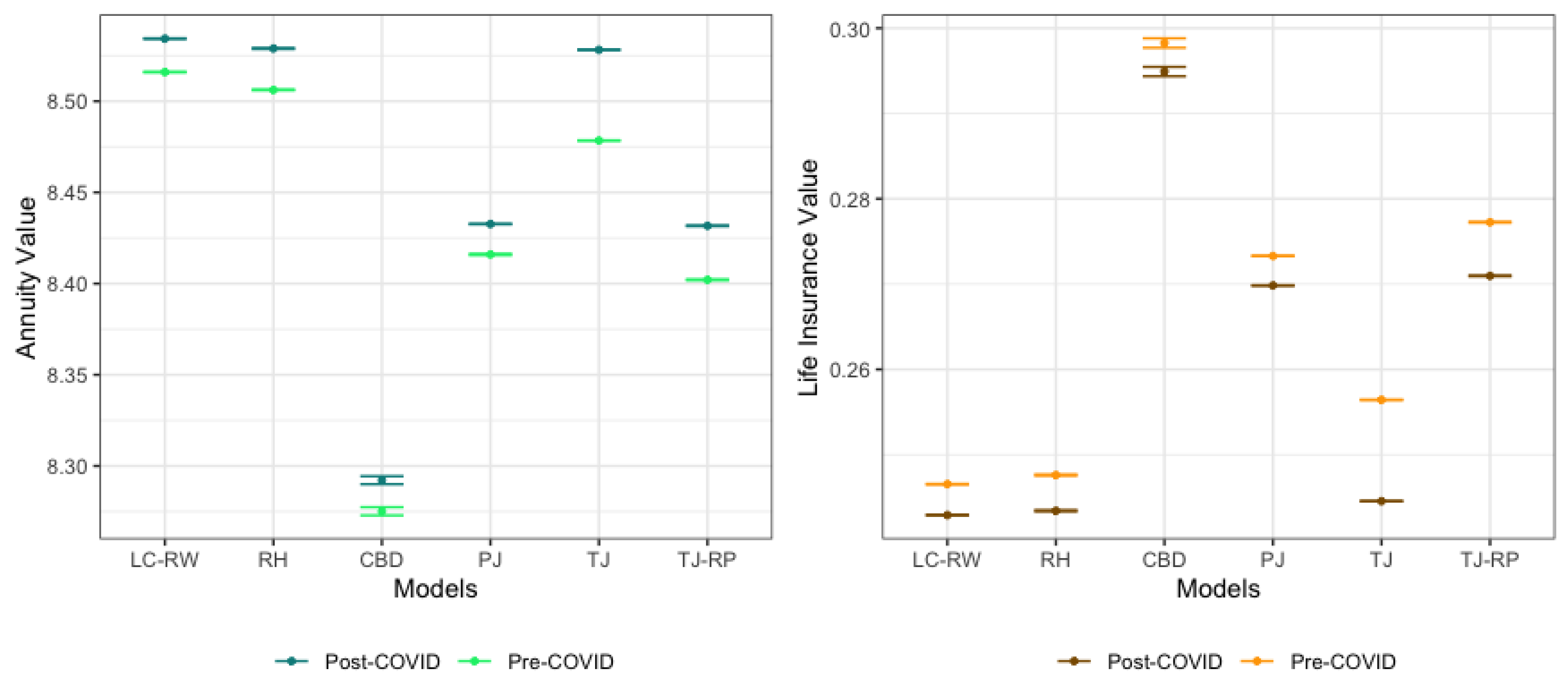
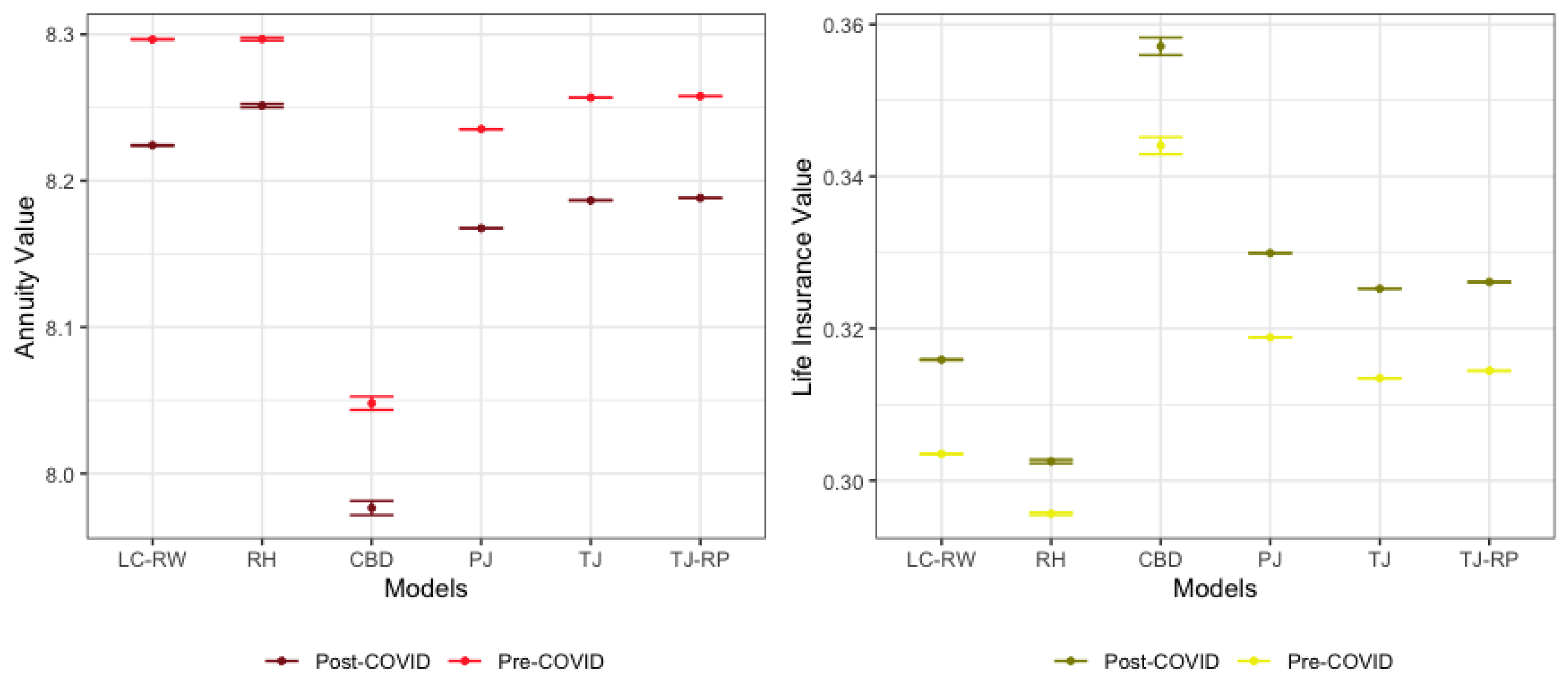
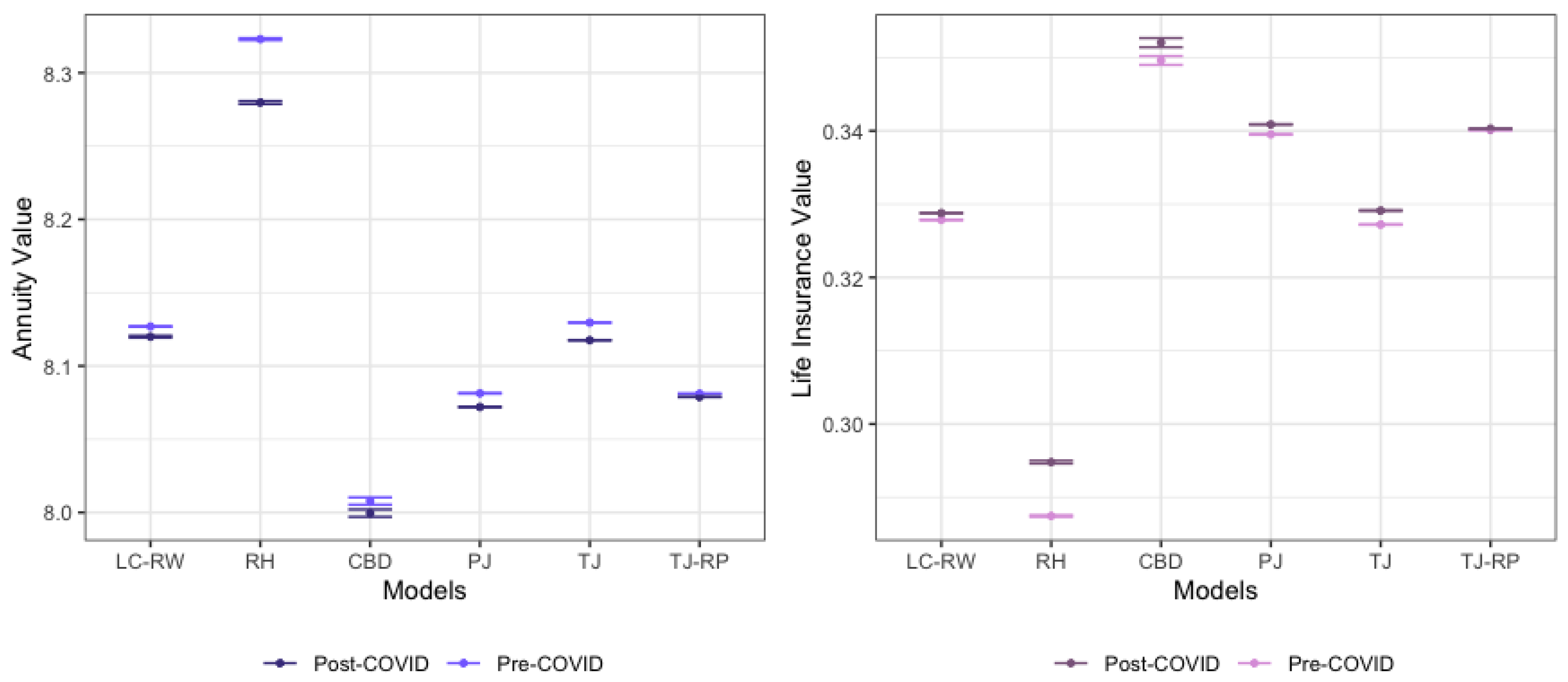
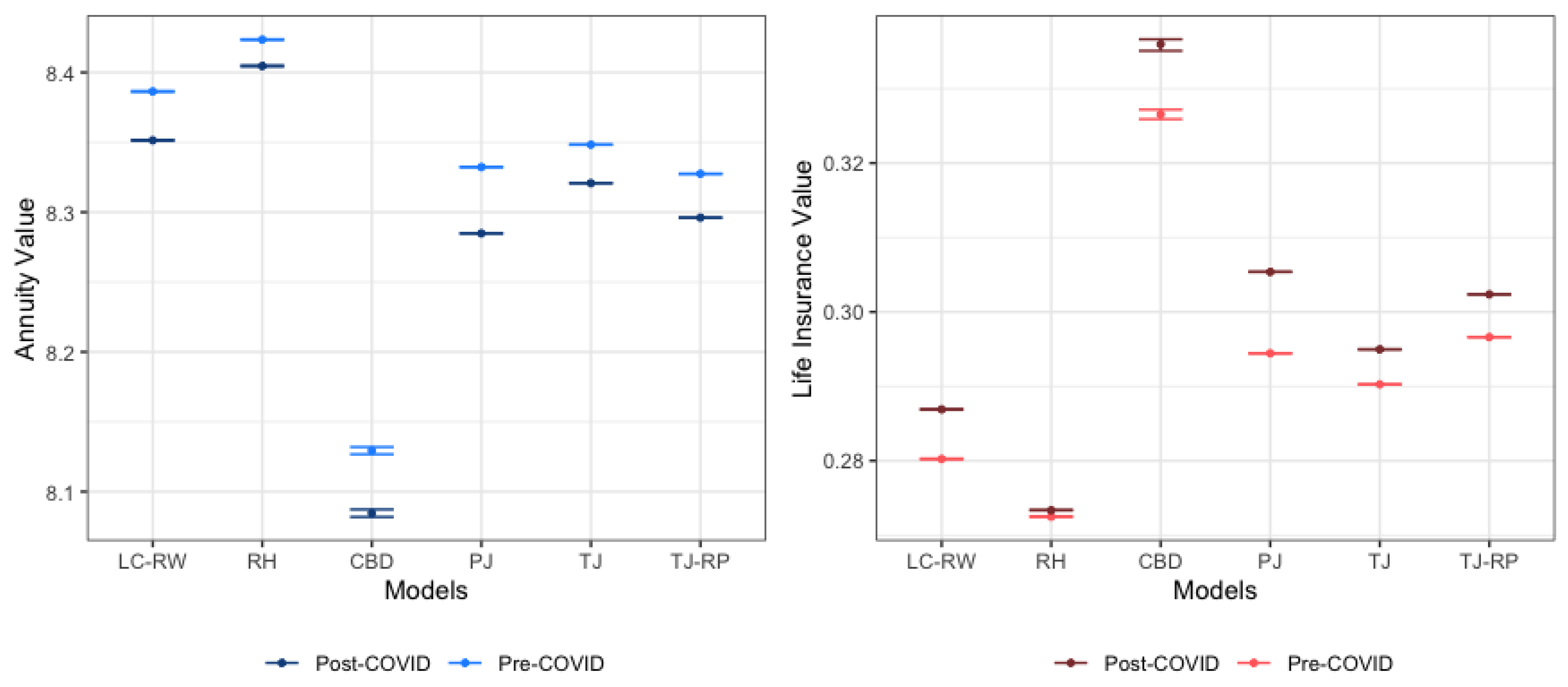
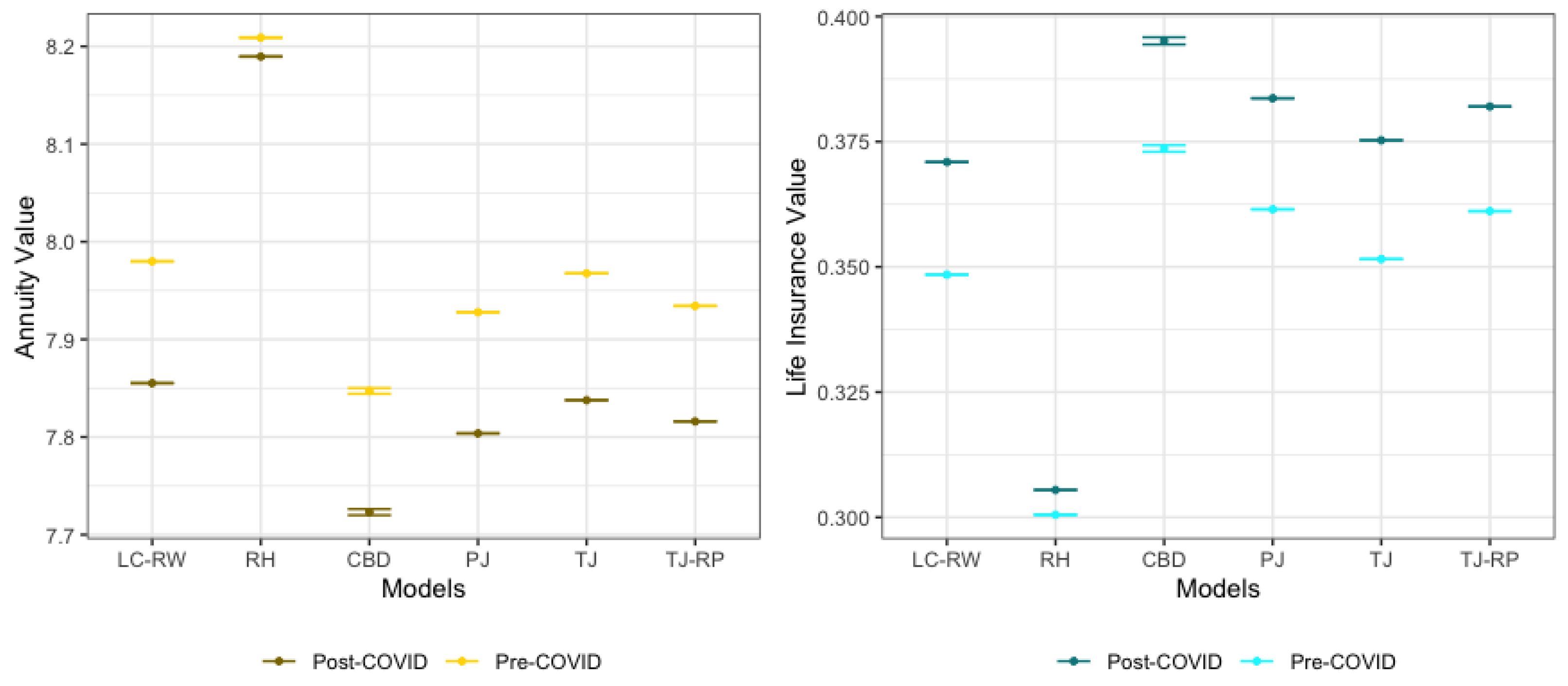
4. Valuation of Mortality-Related Insurance Contracts

In this section, we calibrate the mortality models with and without jump effects for the pre-COVID period (data up to 2019) and the post-COVID period (data up to the latest available year in the HMD, including 2020, 2021, and 2022). Similar to Schnürch et al. (2022), we aim to analyse the impact of the pandemic on the valuation of insurance products, such as term life annuities and life insurance, by using forecasted mortality rates to calculate the present values of the contracts. Since the primary aim is to observe the COVID mortality jumps on forecasted mortality rates and their financial impact on insurance valuation, for simplicity, we use a constant discount factor, v.
First, we consider an n-year term life immediate annuity issued to an individual aged x at the beginning of year t. It pays an amount of 1 at the end of each year in which the annuitant is alive. Denoting p x , t i as the i-year survival probability, the present value of the annuity is given by the following:
α x : n ( t ) = i = 1 n v i i p x , t
= i = 1 n v s s = 0 i 1 p x + s , t + s v i exp s = 0 i 1 η x + s , t + s .
Moreover, we calculate the present value of an n-year term life insurance issued to an individual aged x at the beginning of year t, which pays an amount of 1 at the end of the year if the individual dies within this year, as follows:
A x : n ( t ) = i = 0 n 1 v i i + 1 p x , t ( 1 p x + i , t + i ) i = 0 n 1 v i + 1 exp s = 0 i 1 η x + s , t + s ( 1 exp ( η x + i , t + i ) ) .
where p x , t exp ( η x , t ) is the standard approximation as in Schnürch et al. (2022).
We aim to compare the present values of the life annuities and life insurance for mortality projections calibrated by pre- and post-COVID periods and discuss the differences between the mortality models. For consistency with the previous section, we price a 10-year life insurance and annuity for an individual aged 75.
Figure 2, Figure 3, Figure 4, Figure 5, Figure 6 and Figure 7 show life annuities and life insurance present values along with their 95% confidence intervals. Although results vary from one country to another, there are a few general conclusions that can be drawn. First, post-COVID calibration leads to higher mortality forecasts, which is also evidence that the pandemic does cause a jump, and thus higher life insurance prices along with lower life annuity prices compared to pre-COVID calibration. However, for Japan, the results are the exact opposite. Present values for life annuities for pre-COVID calibration are lower than post-COVID, whilst the present values for life insurance contracts for post-COVID calibration are lower than pre-COVID. The reason is that pre-pandemic mortality in Japan (at least for age 75) is much larger than pandemic and post-pandemic mortality rates as presented in Table 6. Hence, the valuation results are consistent with the mortality results in the previous section. Second, in both insurance contracts, jump models tend to produce similar present values and more or less form clusters in the figures, whilst the jump-free models do not present such a pattern, although LC-RW and RH annuity and life insurance values are close to each other for half of the cases. Third, the CBD model, as in line with the results of the previous sections, produces larger confidence intervals for all countries since we do see the parallel lines for lower and upper confidence levels clearly, although for the other models, they look like one horizontal line. Furthermore, as expected, when there is a significant jump in mortality rates, for example, for Spain in Figure 4 and for the UK in Figure 7, the difference between the pre- and post-COVID calibration periods in the present values of the life annuities and life insurance is larger.

5. Conclusions

This paper aims to analyse the performance of mortality models with and without jump effects in forecasting COVID-19 deaths, the impact of the pandemic on mortality rate forecasts, as well as insurance contract valuations, focusing on the following six countries: Denmark, Japan, Spain, Sweden, Switzerland, and the UK. The comparison of the models involves mortality time indices, κ t , in-sample prediction performances using BIC and MAPE, and out-of-sample forecasting performances based on the simulated forecasted number of deaths for COVID and post-COVID years, while detailed results are discussed throughout the paper, more comprehensive conclusions can be drawn.
One significant observation is that the fit and forecast performance of mortality models, regardless of whether they include jump effects or not, heavily depends on the specific country, time, and age period to which they are fitted. Despite in-sample prediction and model fitting statistics indicating better results for jump models, the forecasting of COVID deaths and death rates for some countries does not support this conclusion. However, by looking at the overall accuracy of the true forecasts for all six countries, the jump models outperform by providing the most accurate forecasts in a majority of the cases. The RH model, having provided the most accurate forecasts for a significant portion of the cases, might be giving insight into future improvements in mortality jump modelling, which indicates considering the age/cohort pattern of the jumps. As mentioned in the relevant section, there is literature on improving the permanent and transitory jump models discussed in this paper. However, when considering the transitory jump model with a renewal process, the extension does not seem straightforward. Since the process of modelling the time-dependent parameter κ t is different and more complex than the other two jump models, it is not possible to add an external age/cohort jump effect on κ t as in Liu and Li (2015). A further research direction might be changing the structure of the model and including the age pattern of mortality jumps in the renewal process setting.
Another observation on the forecasts is that the jump caused by the COVID-19 pandemic, if it indeed occurred, is more visible in older age groups and is reflected in the performance of the jump models specifically designed for them. However, it is crucial to recognise that the sensitivity of the results may vary based on factors such as altering the age range, exploring gender-specific data, or considering a different time frame for analysis.
Considering the findings of the valuation for term life annuities and life insurance, post-COVID calibration results in higher mortality forecasts for all countries except Japan, indicating a pandemic-induced jump and, consequently, lower present values for life annuities and higher present values for life insurance. Jump models exhibit similar present values forming clusters, whereas jump-free models lack such patterns. The CBD model consistently produces larger confidence intervals across all countries.

Author Contributions

Conceptualization, Ş.Ş. and S.Ö.; methodology, Ş.Ş. and S.Ö.; software, Ş.Ş. and S.Ö.; validation, Ş.Ş. and S.Ö.; formal analysis, Ş.Ş. and S.Ö.; investigation, Ş.Ş. and S.Ö.; resources, Ş.Ş. and S.Ö.; data curation, Ş.Ş. and S.Ö.; writing—original draft preparation, Ş.Ş. and S.Ö.; writing—review and editing, Ş.Ş. and S.Ö.; visualization, Ş.Ş. and S.Ö.; supervision, Ş.Ş.; project administration, Ş.Ş.; funding acquisition, Ş.Ş. and S.Ö. All authors have read and agreed to the published version of the manuscript.

Funding

The authors greatly acknowledge partial funding from MAPFRE—Ignacio H. de Larramendi Research Grant 2021.

Data Availability Statement

Mortality data for different countries used in this paper can be obtained from the Human Mortality Database (https://www.mortality.org/).

Conflicts of Interest

The authors declare no conflict of interest.

Appendix A. Transitory Mortality Model with Exponential Jumps and Renewal Process

Table A1. The years of the detected outliers and test statistic values for countries (up to the year of last available data).
DenmarkTime Series ModelARIMA(1,1,0)
(1900–2022)
Year19091921197720112019
JapanTime Series ModelARIMA(0,2,2)
(1947–2021)
Year19491957
SpainTime Series ModelARIMA(1,1,0)
(1908–2021)
Year19181919194219521958201620202021
SwedenTime Series ModelARIMA(1,0,0)
(1908–2019)
Year1917191919201921200320182021
SwitzerlandTime Series ModelARIMA(1,1,0)
(1912–2022)
Year19181919192119231964201620212022
UKTime Series ModelARIMA(1,1,2)
(1922–2021)
Year1931194219442021

Appendix B. Estimated Model Parameters Including COVID Years

Table A2. Estimated model parameters for six countries (up to the year of last available data).
CountryRW without
Jumps
Permanent JumpsTransitory JumpsTransitory Jumps &
Renewal Process
Denmark μ = 1.8045 p = 0.7492 p = 0.8419 μ = 0.5032
(1900–2022) σ = 3.6524 μ = 0.2999 μ = 0.2999 σ = 0.0078
σ = 0.3500 σ = 0.0599 α = 2.9437
m = 5.2843 m = 1.9997 β = 2.2379
s = 1.9999 s = 3.4999 η = 0.4821
BIC = −333.57BIC = −414.61BIC = −319.25BIC = −161.77
MAPE = 62.56MAPE = 16.22MAPE = 15.58MAPE = 14.74
Japan μ = 3.3501 p = 0.4514 p = 0.6325 μ = 0.7498
(1947–2021) σ = 3.4295 μ = 0.6999 μ = 0.7550 σ = 0.0284
σ = 0.3549 σ = 0.3500 α = 8.4291
m = 4.9999 m = 3.8402 β = 7.4542
s = 1.6999 s = 2.1765 η = 0.2969
BIC = −198.36BIC = −279.15BIC = −224.42BIC = −119.25
MAPE = 39.54MAPE = 29.86MAPE = 27.36MAPE = 26.15
Spain μ = 2.2737 p = 0.4637 p = 0.4889 μ = 0.7126
(1908–2021) σ = 5.8078 μ = 0.5498 μ = 0.7500 σ = 0.0356
σ = 0.7500 σ = 0.4499 α = 1.4892
m = 2.9997 m = 0.7499 β = 1.3791
s = 1.2000 s = 0.06492 η = 0.2943
BIC = −363.86BIC = −1111.99BIC = −267.23BIC = −247.34
MAPE = 72.09MAPE = 28.75MAPE = 23.81MAPE = 17.34
Sweden μ = 2.1796 p = 0.6000 p = 0.8419 μ = 0.6997
(1908–2022) σ = 5.4772 μ = 0.6999 μ = 0.5883 σ = 0.0041
σ = 0.6000 σ = 0.0010 α = 0.4312
m = 0.8684 m = 1.9998 β = 0.8330
s = 6.6047 s = 3.0403 η = 0.6586
BIC = −358.00BIC = −373.77BIC = −257.46BIC = −216.69
MAPE = 68.97MAPE = 16.56MAPE = 15.94MAPE = 14.63
Switzerland μ = 2.1005 p = 0.6355 p = 0.5147 μ = 0.6592
(1912–2022) σ = 5.9431 μ = 0.7499 μ = 0.7500 σ = 0.1133
σ = 0.0899 σ = 0.3000 α = 0.6214
m = 3.1617 m = 1.0991 β = 0.7253
s = 1.0999 s = 0.4499 η = 0.5703
BIC = −356.85BIC = −1733.09BIC = −239.34BIC = −223.75
MAPE = 73.87MAPE = 21.81MAPE = 14.18MAPE = 13.06
The UK μ = 1.9556 p = 0.7651 p = 0.5916 μ = 0.7894
(1922–2021) σ = 4.7896 μ = 0.6999 μ = 0.6499 σ = 0.0041
σ = 0.3999 σ = 0.2499 α = 0.4500
m = 2.9998 m = 1.5000 β = 1.0075
s = 1.4999 s = 0.9499 η = 0.4979
BIC = −300.16BIC = −638.11BIC = −265.86BIC = −236.81
MAPE = 62.13MAPE = 34.56MAPE = 16.13MAPE = 13.96

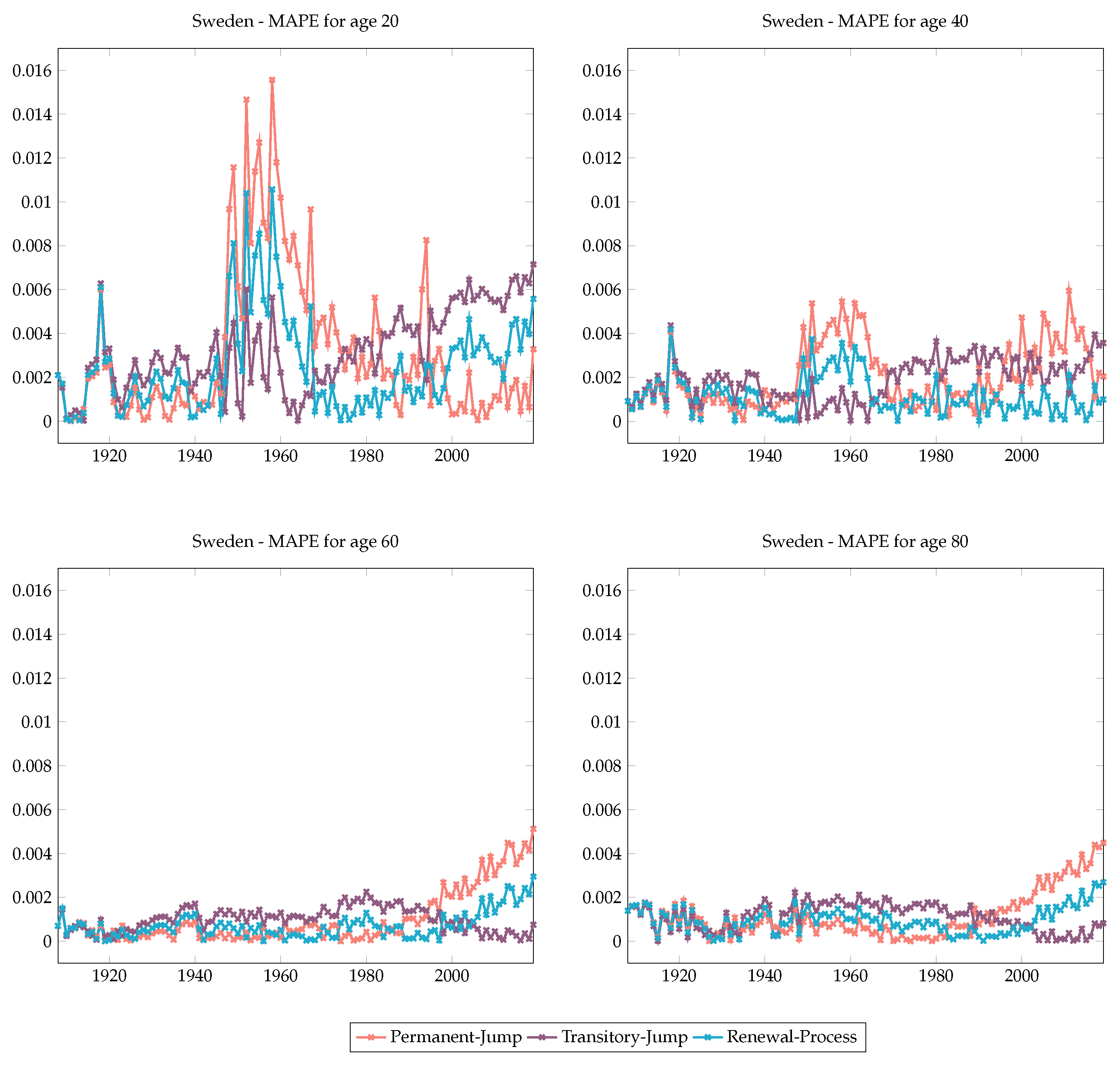
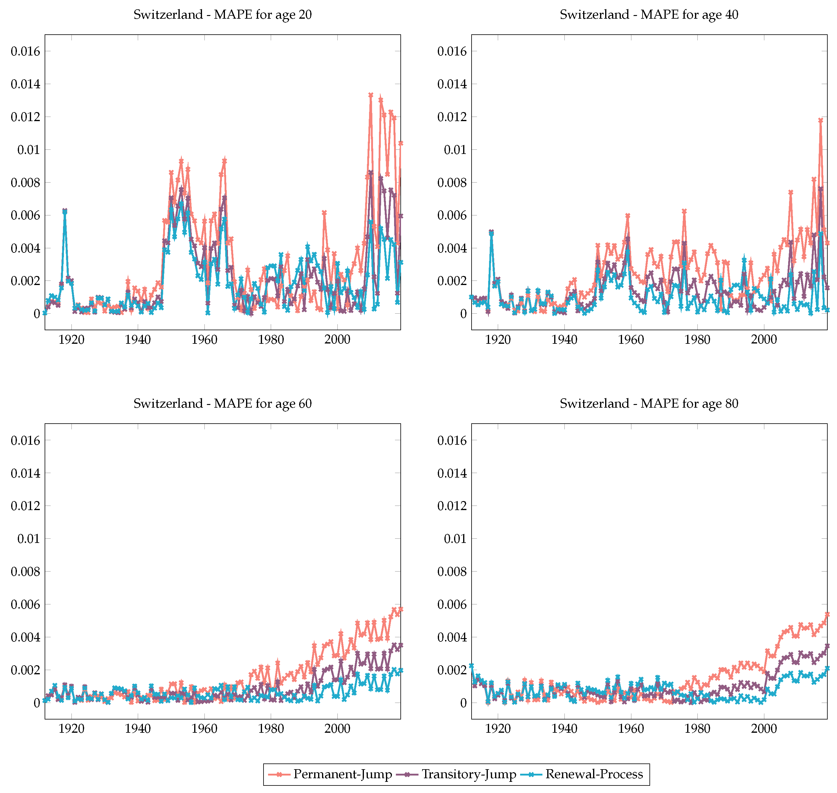
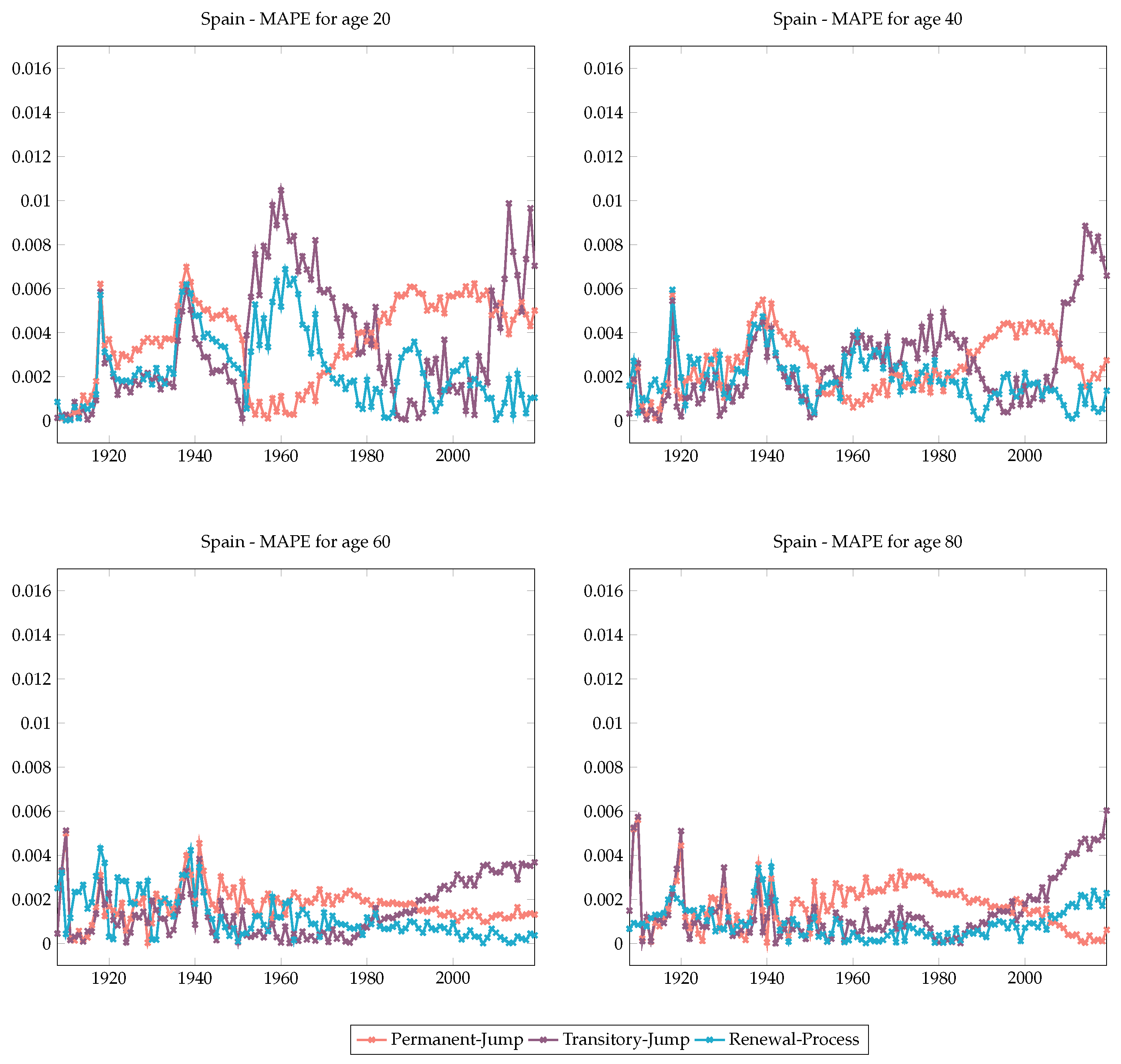
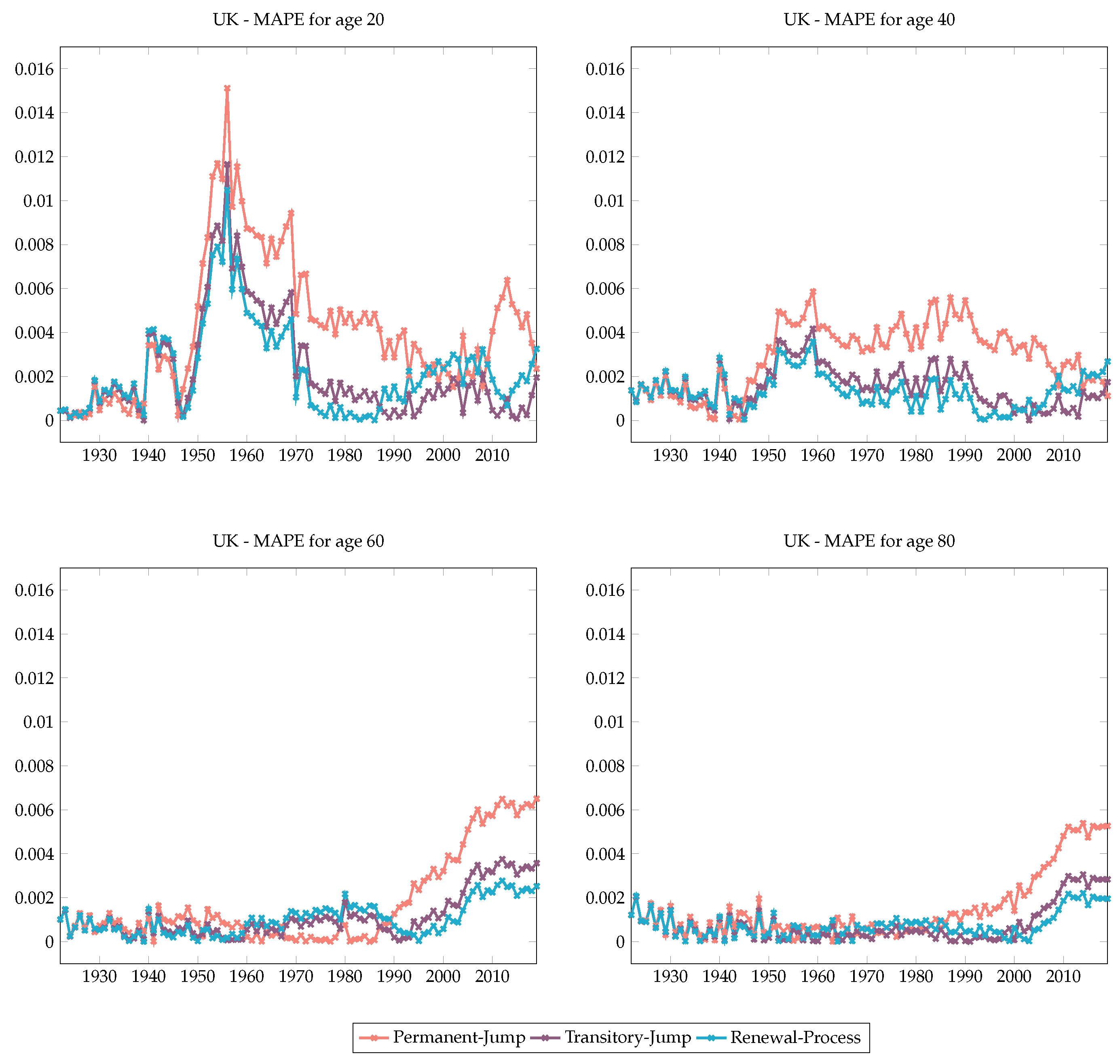
Appendix C. MAPE Values for Different Ages and Mortality Models for Different Countries

Figure A1. MAPE values for different ages and mortality models for Denmark.
Risks 12 00053 g0a1
Figure A2. MAPE values for different ages and mortality models for Japan.
Risks 12 00053 g0a2
Figure A3. MAPE values for different ages and mortality models for Sweden.
Risks 12 00053 g0a3
Figure A4. MAPE values for different ages and mortality models for Switzerland.
Risks 12 00053 g0a4
Figure A5. MAPE values for different ages and mortality models for Spain.
Risks 12 00053 g0a5
Figure A6. MAPE values for different ages and mortality models for UK.
Risks 12 00053 g0a6

References

  1. Brouhns, Natasha, Michel Denuit, and Jeroen K. Vermunt. 2002. A Poisson Log-Bilinear Regression Approach to the Construction of Projected Lifetables. Insurance: Mathematics and Economics 31: 373–93. [Google Scholar] [CrossRef]
  2. Cairns, Andrew J. G. 2023. The Common Cohort Effect Model for Cause of Death Data. “Modelling Measurement and Management of Longevity and Morbidity Risk” research program. London: The Institute and Faculty of Actuaries. [Google Scholar]
  3. Cairns, Andrew J. G., David Blake, and Kevin Dowd. 2006. A Two-Factor Model for Stochastic Mortality with Parameter Uncertainty: Theory and Calibration. Journal of the Risk and Insurance 73: 687–718. [Google Scholar] [CrossRef]
  4. Cairns, Andrew J. G., David Blake, Kevin Dowd, Guy D. Coughlan, Alen Ong, and Igor Balevich. 2007. A Quantitative Comparison of Stochastic Mortality Models Using Data From England and Wales and the United States. North American Actuarial Journal 13: 1–35. [Google Scholar] [CrossRef]
  5. Chen, Hua, and Samuel H. Cox. 2009. Modeling Mortality with Jumps: Applications to Mortality Securitization. The Journal of the Risk and Insurance 3: 727–51. [Google Scholar] [CrossRef]
  6. Chung, Chen, and Lon-Mu Liu. 1993. Joint Estimation of Model Parameters and Outlier Effects in Time Series. Journal of the American Statistical Association 3: 187–211. [Google Scholar]
  7. Cox, Samuel H., Yijia Lin, and Shaun Wang. 2006. Multivariate Exponential Tilting and Pricing Implications for Mortality Securitization. Journal of Risk and Insurance 73: 719–36. [Google Scholar] [CrossRef]
  8. Currie, Iain D., Maria Durban, and Paul H. C. Eilers. 2004. Smoothing and forecasting mortality rates. Statistical Modelling 4: 279–98. [Google Scholar] [CrossRef]
  9. Deng, Yinglu, Patrick L. Brocket, and Richard D. MacMinn. 2012. Longevity/Mortality Risk Modeling and Securities Pricing. The Journal of Risk and Insurance 3: 697–721. [Google Scholar] [CrossRef]
  10. Haberman, Steven, and Arthur E. Renshaw. 2012. Parametric mortality improvement rate modelling and projecting. Insurance: Mathematics and Economics 50: 309–33. [Google Scholar] [CrossRef]
  11. Human Mortality Database. 2023. Available online: https://www.mortality.org (accessed on 1 December 2023).
  12. Li, Ronald D., and Lawrence R. Carter. 1992. Modeling and Forecasting U.S. Mortality. Journal of the American Statistical Association 87: 659–71. [Google Scholar]
  13. Li, Siu-Hang, and Wai-Sum Chan. 2005. Outlier Analysis and Mortality Forecasting: The United Kingdom and Scandinavian Countries. Scandinavian Actuarial Journal 3: 187–211. [Google Scholar] [CrossRef]
  14. Liu, Yanxin, and Johnny S. H. Li. 2015. The Age Pattern of Transitory Mortality Jumps and Its Impact on the Pricing of Catastrophic Mortality Bonds. Insurance: Mathematics and Economics 64: 135–50. [Google Scholar] [CrossRef]
  15. McShane, Blake, Moshe Adrian, Eric T. Bradlow, and Peter S. Fader. 2008. Count Models Based on Weibull Interarrival Times. Journal of Business and Economic Statistics 26: 369–78. [Google Scholar] [CrossRef]
  16. Özen, Selin, and Şule Şahin. 2020. Transitory Mortality Jump Modeling with Renewal Process and Its Impact on Pricing of Catastrophic Bonds. Journal of Computational and Applied Mathematics 376: 112829. [Google Scholar] [CrossRef]
  17. Özen, Selin, and Şule Şahin. 2021. A Two-Population Mortality Model to Assess Longevity Basis Risk. Risks 9: 44. [Google Scholar] [CrossRef]
  18. Regis, Luca, and Petar Jevtic. 2022. Stochastic Mortality Models and Pandemic Shocks. In Pandemics: Insurance and Social Protection. Edited by Maria C. Boado-Penas, Julia Eisenberg and Şule Şahin. Springer Actuarial Series; Cham: Springer, pp. 61–73. [Google Scholar]
  19. Renshaw, Arthur E., and Steven Haberman. 2003. Lee–Carter Mortality Forecasting with Age-Specific Enhancement. Insurance: Mathematics and Economics 33: 255–72. [Google Scholar] [CrossRef]
  20. Renshaw, Arthur E., and Steven Haberman. 2006. A Cohort-Based Extension to the Lee–Carter Model for Mortality Reduction Factors. Insurance: Mathematics and Economics 38: 556–70. [Google Scholar] [CrossRef]
  21. Richards, Stephan J. 2023. Robust Mortality Forecasting in the Presence of Outliers. Presented to the Faculty of Actuaries. Edinburgh: Longevitas Ltd., pp. 1–28. [Google Scholar]
  22. Schnürch, Simon, Torsten Kleinow, and Andreas Wagner. 2023. Accounting for COVID-19-type shocks in mortality modeling: A comparative study. Journal of Demographic Economics 89: 483–512. [Google Scholar] [CrossRef]
  23. Schnürch, Simon, Torsten Kleinow, Ralf Korn, and Andreas Wagner. 2022. The impact of mortality shocks on modelling and insurance valuation as exemplified by COVID-19. Annals of Actuarial Science 16: 498–526. [Google Scholar] [CrossRef]
  24. Venter, Gary. 2022. A Mortality Model for Pandemics and Other Contagion Events. In Pandemics: Insurance and Social Protection. Edited by Maria C. Boado-Penas, Julia Eisenberg and Şule Şahin. Springer Actuarial Series; Cham: Springer, pp. 75–94. [Google Scholar]
  25. Villegas, Andres M., Pietro Millossovich, and Vladimir K. Kaishev. 2018. StMoMo: Stochastic Mortality Modeling in R. Journal of Statistical Software 84: 1–38. [Google Scholar] [CrossRef]
Figure 1. κ t Parameters for LC and mortality jump models for different countries.
Risks 12 00053 g001
Figure 2. Present values of term life annuity and life insurance contracts using Denmark mortality data.
Risks 12 00053 g002
Figure 3. Present values of term life annuity and life insurance contracts using Japan mortality data.
Risks 12 00053 g003
Figure 4. Present values of term life annuity and life insurance contracts using Spain mortality data.
Risks 12 00053 g004
Figure 5. Present values of term life annuity and life insurance contracts using Sweden mortality data.
Risks 12 00053 g005
Figure 6. Present values of term life annuity and life insurance contracts using Switzerland mortality data.
Risks 12 00053 g006
Figure 7. Present values of term life annuity and life insurance contracts using UK mortality data.
Risks 12 00053 g007
Table 1. The years of the detected outliers and the time series models of the mortality indices for the countries (up to 2019).
DenmarkTime Series ModelARIMA(1,1,0) MAPE46.14
(1900–2019)
Years19091921197720112019
JapanTime Series ModelARIMA(0,2,2) MAPE90.97
(1947–2019)
Years19491957
SpainTime Series ModelARIMA(1,1,0) MAPE44.82
(1908–2019)
Years1918191919421952195819722016
SwedenTime Series ModelARIMA(1,0,0) MAPE49.91
(1908–2019)
Years1917191919201921200320182019
SwitzerlandTime Series ModelARIMA(1,1,0) MAPE38.75
(1912–2019)
Years1918191919211923195019642016
UKTime Series ModelARIMA(1,1,2) MAPE48.16
(1922–2019)
Years193119421944
Table 2. Estimated MAPE values for κ t parameters for six countries (up to 2019).
Country Permanent Jumps Transitory Jumps Transitory Jumps & Renewal Process
Denmark 1.4054 1.0077 0.3170
Japan 2.0522 2.7480 1.8036
Spain 3.0178 1.1210 0.4981
Sweden 0.9383 2.6750 0.7685
Switzerland 0.6871 0.2040 0.2951
The UK 0.9079 0.3451 0.5801
Table 3. Estimated model parameters for six countries (up to 2019).
CountryLC-RWPermanent JumpsTransitory JumpsTransitory Jumps &
Renewal Process
Denmark μ = 1.9014 p = 0.6704 p = 0.8484 μ = 0.2016
(1900–2019) σ = 3.6579 μ = 0.2999 μ = 0.2492 σ = 0.0066
σ = 0.4500 σ = 0.0005 α = 0.4062
m = 5.3217 m = 2.2926 β = 0.4095
s = 1.6999 s = 3.4992 η = 1.6920
BIC = −327.96BIC = −442.84BIC = −310.67BIC = −52.49
Japan μ = 3.4238 p = 0.2668 p = 0.5781 μ = 0.6840
(1947–2019) σ = 3.4061 μ = 0.7998 μ = 0.8549 σ = 0.0162
σ = 0.4549 σ = 0.3548 α = 7.53763
m = 4.9992 m = 2.6991 β = 8.23064
s = 0.6998 s = 1.0999 η = 0.29636
BIC = −194.69BIC = −524.00BIC = −253.92BIC = −114.70
Spain μ = 2.4130 p = 0.3239 p = 0.4921 μ = 0.7110
(1908–2019) σ = 5.1468 μ = 0.4499 μ = 0.8001 σ = 0.0926
σ = 0.7549 σ = 0.3999 α = 1.9484
m = 2.4999 m = 0.6500 β = 1.4574
s = 0.8999 s = 0.0549 η = 0.2959
BIC = −344.09BIC = −1193.27BIC = −337.24BIC = −227.74
Sweden μ = 2.670 p = 0.6000 p = 0.7538 μ = 0.7452
(1908–2019) σ = 5.1981 μ = 0.6994 μ = 0.7000 σ = 0.0185
σ = 0.5500 σ = 0.1330 α = 1.9716
m = 0.7211 m = 1.9999 β = 1.9802
s = 6.2341 s = 2.9406 η = 0.4699
BIC = −345.18BIC = -366.61BIC = −254.07BIC = −181.07
Switzerland μ = 2.2020 p = 0.7128 p = 0.5078 μ = 0.6593
(1912–2019) σ = 5.7835 μ = 0.7996 μ = 0.6499 σ = 0.2663
σ = 0.3499 σ = 0.2997 α = 0.6202
m = 3.1989 m = 1.0999 β = 0.7061
s = 1.4999 s = 0.4499 η = 0.5949
BIC = −344.30BIC = −933.11BIC = −251.97BIC = −216.12
The UK μ = 2.1735 p = 0.5326 p = 0.7839 μ = 0.8811
(1922–2019) σ = 4.3416 μ = 0.7997 μ = 0.7500 σ = 0.0363
σ = 0.5499 σ = 0.1179 α = 1.9436
m = 0.9996 m = 1.3999 β = 1.8884
s = 0.7000 s = 2.2849 η = 0.4961
BIC = −282.35BIC = −1329.75BIC = −202.59BIC = −160.36
Table 4. BIC and MAPE Values of all models for six countries (up to 2019).
CountryLC-RWRHCBDPermanent JumpsTransitory JumpsTransitory Jumps &
Renewal Process
Denmark
(1900–2019)
BIC−2,507,517−12,625,099−1,438,469−201,649.80−153,532.60−87,829.99
MAPE62.8883.5448.5823.8320.1214.45
Japan
(1947–2019)
BIC−9,185,253−123,725,040−8,915,135−3,577,544−1,416,897−1,316,616
MAPE39.12107.5839.4829.5827.6225.57
Spain
(1908–2019)
BIC−30,767,472−81,396,057−16,432,829−3,162,232−1,661,928−1,503,534
MAPE70.2085.7767.9129.6528.5717.90
Sweden
(1908–2019)
BIC−4,805,222−23,712,707−1,462,889−198,654.20−185,479.60−130,953.20
MAPE68.7196.7237.1721.7520.5814.40
Switzerland
(1912–2019)
BIC−5,164,856−23,625,717−1,099,357−178,031−106,925.90−83,879.52
MAPE73.32240.1940.0926.5516.8612.82
The UK
(1922–2019)
BIC−21,466,019−223,085,156−9,488,580−1,255,758−487,732.40−413,783.10
MAPE60.82102.7636.0127.4414.3513.85
Table 5. Comparison of number of deaths in Denmark for age 75.
CountryFitting
Years
Estimation
Years
Number of
Deaths
ModelsQuantiles
0 % 25 % 50 % 75 % 100 % Range
(Max–Min)
Denmark1908–201920191626LC-RW
20201706 1621.181744.511767.261789.931918.09296.91
20211694 1695.291824.261848.041871.752005.77310.48
20221810 1671.201798.331821.781845.141977.26306.07
RH Model
20201706 1566.561668.901691.561715.901796.69230.12
20211694 1586.521715.751752.281787.911911.63325.12
20221810 1501.651643.751687.701729.131883.70382.05
CBD
Model
20201706 1450.231778.391848.161925.842285.08834.85
20211694 1356.641841.021947.102056.252648.281291.65
20221810 1266.581803.291927.642066.763051.361784.78
Permanent
Jump
20201706 1701.901760.591776.491812.321833.70131.80
20211694 1794.541856.431873.191910.971933.52138.97
20221810 1783.791845.311861.971899.521921.94138.14
Transitory
Jump
20201706 1631.421744.151768.561782.461902.55271.14
20211694 1703.461821.171846.661861.171986.57283.11
20221810 1676.761792.621817.711831.991955.43278.67
Transitory
Jump &
Renewal
Process
20201706 1660.491786.181798.321813.641973.36312.87
20211694 1769.201903.111916.051932.362102.55333.35
20221810 1776.991911.501924.491940.882111.82334.82
Table 6. Comparison of number of deaths in Japan for age 75.
CountryFitting
Years
Estimation
Years
Number of
Deaths
ModelsQuantiles
0 % 25 % 50 % 75 % 100 % Range
(Max–Min)
Japan1908–2019201929,155
LC-RW
202024,872 21,699.0424,043.4724,483.2624,923.8127,456.245757.20
202121,721 19,085.5421,147.6021,534.4221,921.9024,149.325063.78
RH Model
202024,872 24,294.9824,690.1324,775.1624,865.6025,158.96863.98
202121,721 23,598.6324,420.0924,699.8524,964.6225,369.291770.66
CBD
Model
202024,872 24,681.3627,674.0728,495.5029,401.6932,135.477454.11
202121,721 21,094.4024,446.4925,595.2326,712.2031,410.1110,315.71
Permanent
Jump
202024,872 23,673.7224,540.8525,208.5225,287.3425,603.971930.25
202121,721 21,256.4522,035.0322,634.5322,705.3022,989.601733.15
Transitory
Jump
202024,872 23,598.6324,420.0924,699.8524,964.6225,369.291770.66
202121,721 20,921.0021,649.2521,897.2722,132.0022,490.741569.74
Transitory
Jump &
Renewal
Process
202024,872 18,610.9624,552.9925,010.2025,477.1633,364.0914,753.13
202121,721 16,724.1922,063.8122,474.6622,894.2929,981.6513,257.46
Table 7. Comparison of number of deaths in Spain for age 75.
CountryFitting
Years
Estimation
Years
Number of
Deaths
ModelsQuantiles
0 % 25 % 50 % 75 % 100 % Range
(Max–Min)
Spain1908–201920198036
LC-RW
20209662 6492.157530.467730.477932.429123.902631.75
20218868 6478.527514.657714.237915.769104.742626.22
RH Model
20209662 6990.118089.898318.558551.439759.312769.20
20218868 6582.577926.648246.598565.3510,468.823886.25
CBD
Model
20209662 7263.439490.0610,044.1010,653.0113,502.916239.48
20218868 6347.469403.3510,195.6011,066.7216,026.089678.62
Permanent
Jump
20209662 7480.597791.207865.867907.208067.95587.36
20218868 7575.637890.187965.798007.668170.45594.82
Transitory
Jump
20209662 7674.477783.177804.817826.347915.62241.16
20218868 7732.777842.307864.117885.807975.76243.00
Transitory
Jump &
Renewal
Process
20209662 6983.007740.117792.547823.828630.571647.57
20218868 7012.477772.777825.427856.838666.991654.52
Table 8. Comparison of number of deaths in Sweden for age 75.
CountryFitting
Years
Estimation
Years
Number of
Deaths
ModelsQuantiles
0 % 25 % 50 % 75 % 100 % Range
(Max–Min)
Sweden1908–201920192333
LC-RW
20202565 2292.492533.122578.192623.312882.30589.81
20212474 2292.792533.462578.532623.662882.68589.89
20222363 2266.272504.152548.712593.312849.34583.07
RH Model
20202565 2281.032331.332344.342358.402406.55125.52
20212474 2252.262316.402334.742354.902427.10174.83
20222363 2171.522245.502267.202288.412370.01198.49
CBD
Model
20202565 2302.352688.602769.432857.393255.75953.40
20212474 2115.582672.462788.392905.833515.221399.64
20222363 2015.342630.632768.922921.123964.051399.64
Permanent
Jump
20202565 2284.332580.002593.842619.822946.18661.85
20212474 2302.682600.732614.672640.862969.85667.17
20222363 2294.032590.952604.842630.932958.68664.66
Transitory
Jump
20202565 2418.952556.072588.302599.302728.74309.79
20212474 2420.082557.272589.512600.522730.02309.94
20222363 2392.892528.542560.412571.302699.34306.45
Transitory
Jump &
Renewal
Process
20202565 2429.932582.632592.952599.762754.19324.26
20212474 2442.432595.912606.292613.132768.36325.93
20222363 2426.272578.742589.052595.852750.05323.78
Table 9. Comparison of number of deaths in Switzerland for age 75.
CountryFitting
Years
Estimation
Years
Number of
Deaths
ModelsQuantiles
0 % 25 % 50 % 75 % 100 % Range
(Max–Min)
Switzerland1908–201920191436
LC-RW
20201607 1334.221583.491632.141681.471976.30642.10
20211540 1351.001603.411652.681702.632001.17650.20
20221571 1340.451590.881639.761689.321985.53645.10
RH Model
20201607 1346.291425.051447.221468.091559.83213.50
20211540 1308.421418.551446.461476.901612.00303.60
20221571 1291.431426.181464.131500.611678.52387.10
CBD
Model
20201607 1441.971699.351755.471814.772093.26651.30
20211540 1336.121715.811794.801877.062305.43969.30
20221571 1287.481700.381795.571899.352626.871339.40
Permanent
Jump
20201607 1561.121630.641648.381675.001717.65156.50
20211540 1597.921669.081687.231714.461758.14160.20
20221571 1602.641674.011692.211719.531763.33160.70
Transitory
Jump
20201607 1611.281637.601646.441651.731668.1056.82
20211540 1644.181671.031680.051685.451702.1657.98
20221571 1643.941670.801679.811685.221701.9157.97
Transitory
Jump &
Renewal
Process
20201607 1460.021636.641648.651659.091831.28371.26
20211540 1492.681673.241685.521696.201872.24379.56
20221571 1495.321676.201688.501699.201875.55380.23
Table 10. Comparison of number of deaths in the UK for age 75.
CountryFitting
Years
Estimation
Years
Number of
Deaths
ModelsQuantiles
0 % 25 % 50 % 75 % 100 % Range
(Max–Min)
UK1908–2019201914,170
LC-RW
202015,992 13,686.8815,158.5615,434.5515,711.0017,299.713612.80
202115,549 13,237.8714,661.2714,928.2115,195.5816,732.183494.30
RH Model
202015,992 13,241.5413,596.6113,673.8813,750.6814,134.80893.30
202115,549 12,585.8013,003.1713,110.2013,212.9813,675.611089.80
CBD
Model
202015,992 13,533.4615,975.0516,515.7617,098.2719,717.186183.70
202115,549 12,018.1715,377.8416,117.6616,900.1720,921.388903.20
Permanent
Jump
202015,992 15,190.8515,508.8115,574.3715,625.6215,885.62694.80
202115,549 14,816.6215,126.7515,190.7015,240.6915,494.28677.70
Transitory
Jump
202015,992 14,557.6315,334.8815,511.3515,576.9316,327.321769.70
202115,549 14,108.8914,862.1915,033.2215,096.7815,824.031715.10
Transitory
Jump &
Renewal
Process
202015,992 14,443.3215,452.8915,523.1415,567.8716,596.262152.90
202115,549 14,037.5915,018.8015,087.0815,130.5616,130.062092.50
Disclaimer/Publisher’s Note: The statements, opinions and data contained in all publications are solely those of the individual author(s) and contributor(s) and not of MDPI and/or the editor(s). MDPI and/or the editor(s) disclaim responsibility for any injury to people or property resulting from any ideas, methods, instructions or products referred to in the content.

