Bounds for the Ruin Probability in the Sparre–Andersen Model

Abstract

We obtain the upper and lower bounds for the ruin probability in the Sparre–Andersen model. These bounds are established under various conditions: when the adjustment coefficient exists, when it does not exist, and when the interarrival distribution belongs to certain aging classes. Additionally, we improve the Lundberg upper bound for the ruin probability.

1. Introduction

In actuarial science and insurance, the Sparre–Andersen risk model plays a crucial role in stochastically modelling a company’s surplus or its available financial resources over time. This model generalises the classical risk model that was introduced by Lundberg (see, e.g., Asmussen and Albrecher (2010); Schmidli (2017); Rolski et al. (1999)), assuming that the claim number process is a renewal process (see, e.g., Labbé and Sendova (2009); Li and Garrido (2005); Temnov (2004, 2014); Willmot (2007); Asmussen and Albrecher (2010)). This model has recently become a focal point for research. A key area of interest is the ruin probability, which essentially means the probability of the company’s surplus turning negative at some point. The complexity of this concept means that there is no straightforward formula for calculating this probability. As a result, researchers are engaged in developing approximations, bounds, and asymptotic formulas to better grasp its characteristics.

In this paper, we will present both the upper and lower bounds for the ruin probability. Specifically, after a mathematical overview of the Sparre–Andersen model, we will present the proof of certain lemmas that will assist us in establishing the proof of the aforementioned bounds. Initially, we will focus on the upper and lower bounds in the case where the adjustment coefficient exists, with the upper bound being a refined version of Lundberg’s famous inequality. Moreover, these bounds serve as enhancements to those previously given by Psarrakos and Politis (2009a). Next, we will provide bounds for the ruin probability, using properties from aging classes for the distribution of the claim amounts. Our work offers enhancements to the bounds proposed by Willmot et al. (2001); Willmot (2002); Psarrakos and Politis (2009a). Finally, we will generalize the conditions under which the bounds proposed by Chadjiconstantinidis and Xenos (2022), for the cases where the adjustment coefficient does not exist, can be applied.

2. Model Description

Consider the Sparre–Andersen risk model for an insurance surplus process defined as

$$U\left(t\right)=u+ct-\sum _{k=1}^{N_t}{Y}_k$$

is the surplus at time t, where u$(\ge 0)$ is the surplus at time $t=0$ (also known as the initial surplus) and c is the rate of premium income per unit of time. With $N_t$, we denote the number of claims in the time interval $(0,t]$. The individual claim amounts $Y_i$ ($i=1,2,\dots$) are independent, identically distributed (i.i.d.) non-negative random variables with a common distribution function (d.f.) $P\left(t\right)=Pr\left(Y_1\le t\right)$, tail $\overline{P}\left(t\right)=1-P\left(t\right)$, density $p\left(t\right)$ and mean $E\left(Y_1\right)=m<\infty$. The claim amounts are also independent of $N_t$, and the corresponding interclaim times $W_1,W_2,\dots$ are i.i.d. with common mean $E\left(T_1\right)$. Also, we assume that $c=(1+\theta )m/E\left(T_1\right)$, where $\theta >0$ is the implied relative security loading. Also, F is the distribution of the drop in the surplus given that such a drop occurs (see, e.g., Willmot (2002)).

Now, let $T=inf\{t\ge 0:U(t)<0\}$ be the time of ruin, then the ruin probability is defined as

$$\psi \left(u\right)=\mathbb{P}(T<\infty \mid U(0)=u).$$

The probability of ruin $\psi \left(u\right)$ satisfies the defective renewal equation (see, e.g., Willmot and Lin (2001) and Section 3.2)

$$\psi \left(u\right)=\varphi \overline{F}\left(u\right)+\varphi {\int }_0^u\psi (u-t)dF\left(t\right),$$

(1)

with solution

$$\psi \left(u\right)=\varphi \overline{F}\left(u\right)+\frac{\varphi }{1-\varphi }{\int }_0^u\overline{F}(u-t)dH\left(t\right),$$

(2)

where

$$H\left(u\right)=1-\psi \left(u\right)=\sum _{n=0}^{\infty }(1-\varphi ){\varphi }^n{F}^{\ast n}\left(u\right)$$

is the probability of non-ruin, $\varphi =\psi \left(0\right)$, $0<\varphi <1$ and $\overline{F^{\ast n}}\left(u\right)=1-F^{\ast n}\left(u\right)$ is the tail of the n-fold convolution of the ladder height distribution F associated with the risk process.

The solution to Equation (1) is given by the Pollaczek–Khintchine type formula,

$$\psi \left(u\right)=\sum _{m=1}^{\infty }(1-\varphi ){\varphi }^m{\overline{F}}^{\ast m}\left(u\right),$$

(3)

i.e., $\psi \left(u\right)$ is a geometric compound tail with geometric parameter $\varphi$ (see, e.g., Willmot and Woo (2017)).

One of the primary results in the study of ruin probabilities is Lundberg inequality, namely:

$$\psi \left(u\right)\le e^{-Ru},$$

where R is called the adjustment coefficient and is defined as the unique positive solution of the following equation

$${\int }_0^{\infty }{e}^{Rx}dF\left(x\right)=\frac{1}{\varphi }.$$

(4)

The last equation is known as the Lundberg condition, and integrating by parts the above gives

$${\int }_0^{\infty }{e}^{Rx}\overline{F}\left(x\right)dx=\frac{1-\varphi }{\varphi R}.$$

(5)

Another key result is the Cramer–Lundberg asymptotic formula:

$$\underset{u\to \infty }{lim}{e}^{Ru}\psi \left(u\right)=C,$$

where

$$C=\frac{1-\varphi }{\varphi R{\int }_0^{\infty }x{e}^{Rx}dF\left(x\right)}.$$

There are numerous distributions which do not satisfy (4) (see Cai and Garrido (1998); Chadjiconstantinidis and Xenos (2022)). For this case Dickson (1994) considered a truncating version of (4), i.e., suppose that for any given $t\ge 0$, there exists a constant $R_{\varphi }\left(t\right)\ge 0$, such that

$${\int }_0^t{e}^{x{R}_{\varphi }\left(t\right)}dF\left(x\right)=\frac{1}{\varphi }.$$

In actuarial risk theory, a key variable of interest introduced by Gerber et al. (1987), is the deficit at ruin, with distribution defined as

$$H(u,y)=\mathbb{P}\left(\right|U\left(T\right)|\le y,T<\infty |U\left(0\right)=u).$$

It is a defective distribution function with a right tail:

$$\overline{H}(u,y)=\psi \left(u\right)-H(u,y).$$

This satisfies the following defective renewal equation

$$\overline{H}(u,y)=\varphi \overline{F}(u+y)+\varphi {\int }_0^u\overline{H}(u-t,y)dF\left(t\right),$$

(6)

with solution

$$\overline{H}(u,y)=\varphi \overline{F}(u+y)+\frac{\varphi }{1-\varphi }{\int }_0^u\overline{F}(u+y-t)dH\left(t\right).$$

3. Definitions, Notation and Preliminary Results

This section outlines all the mathematical tools we will use in subsequent sections to introduce new bounds for the ruin probability in the Sparre–Andersen risk model.

3.1. Definitions and Notation

We denote by $h\left(u\right)$ the quantity

$$h\left(u\right)=\psi \left(u\right)-e^{-Ru},u\ge 0.$$

(7)

We also define

$$G\left(u\right)=1-\overline{G}\left(u\right)=\frac{{\int }_0^u{e}^{Rt}dF\left(t\right)}{{\int }_0^{\infty }{e}^{Rt}dF\left(t\right)}=\varphi {\int }_0^u{e}^{Rt}dF\left(t\right),u\ge 0.$$

(8)

and the function ${\mathsf{\Lambda }}_u\left(y\right)$

$${\mathsf{\Lambda }}_u\left(y\right)=\frac{\varphi }{1-\varphi }\left(\psi (u+y)-\psi \left(u\right)\psi \left(y\right)\right),u,y\ge 0,$$

(9)

that serves as a critical component in the proof of Proposition 2.

And lastly, for convenience in algebraic manipulation, we define

$$\xi \left(u\right)=\varphi \overline{F}\left(u\right)-e^{-Ru}\overline{G}\left(u\right),u\ge 0.$$

(10)

3.2. Convolutions and Renewal Equation

For two integrable functions $f,g$ their convolution $f\ast g$ is defined by

$$(f\ast g)\left(t\right)={\int }_0^{t}f(t-x)g\left(x\right)dx,$$

while for two distribution functions $F,G$ the convolution $F\ast G$ is defined by $(F\ast G)\left(t\right)={\int }_0^{t}F(t-x)dG\left(x\right)$. In either case, the symbol $f^{\ast \left(k\right)}$ ($F^{\left(k\right)}$) denotes the kth convolution product of f (resp., F) by itself.

Generally, an equation with the following form

$$Z\left(t\right)=z\left(t\right)+\varphi {\int }_0^{t}Z(t-x)dF\left(x\right),$$

for $0<\varphi <1$ is called a defective renewal type equation and is known to have the following unique solution (see, e.g., Willmot and Lin (2001) for a detailed discussion of the solution of the defective renewal equation)

$$Z\left(t\right)=z\left(t\right)+\frac{1}{1-\varphi }{\int }_0^{t}z(t-x)dU\left(x\right),$$

(11)

where

$$U\left(x\right)=\sum _{k=0}^{\infty }{\varphi }^k{F}^{\ast k}\left(x\right).$$

3.3. Aging Classes

This section introduces the aging classes that we will utilize in Section 4.2 (see, e.g., Willmot and Lin (2001)). Each aging class contains distributions characterised by particular failure rate properties. These classes have been developed within the field of reliability theory and survival analysis to analyze respective lifespans. Furthermore, these classes are applied in actuarial science and insurance, aiding in the modelling of claim amounts and the number of claims. The classes used here include IFR (DFR), NBU (NWU) and NBUC (NWUC).

The d.f. $F\left(y\right)$ is said to be decreasing (increasing) failure rate or DFR (IFR) if $\overline{F}(x+y)/\overline{F}\left(y\right)$ is nondecreasing (nonincreasing) in y for fixed $x\ge 0$, i.e., if $\overline{F}\left(y\right)$ is log-convex (log-concave). Also, if $F\left(y\right)$ is absolutely continuous, then DFR (IFR) is equivalent to $\lambda \left(y\right)$ nonincreasing (nondecreasing) in y, where $\lambda \left(y\right)=f\left(y\right)/\overline{F}\left(y\right)$.

A d.f. $F\left(y\right)$ is called new worse (better) than used or NWU (NBU) if

$$\overline{F}(x+y)\ge (\le )\overline{F}\left(x\right)\overline{F}\left(y\right),\mathrm{for}\mathrm{all}x,y\ge 0.$$

Another class is the new worse (better) than used in convex ordering or NWUC (NBUC) class. The d.f. $F\left(y\right)$ is NWUC (NBUC) if

$${\overline{F}}_e(x+y)\ge (\le ){\overline{F}}_e\left(y\right)\overline{F}\left(x\right),$$

for all $x,y\ge 0$ and $F_e\left(x\right)=1/\mu {\int }_0^x\overline{F}\left(t\right)dt$ is the equilibrium distribution of F.

3.4. Preliminary Results

This section introduces four Lemmas and a Proposition, which are crucial for the proof of the bounds for the ruin probability. In the following result, we present a renewal-type equation for the difference $h\left(u\right)=\psi \left(u\right)-e^{-Ru}$.

Lemma 1.

The function h(u) satisfies the following renewal equation

$$h\left(u\right)=\varphi \overline{F}\left(u\right)-e^{-Ru}\overline{G}\left(u\right)+\varphi {\int }_0^{u}h(u-x)dF\left(x\right),u\ge 0.$$

(12)

Proof. 

Substituting (7) and (8) into (1) we have:

$$h\left(u\right)+e^{-Ru}=\varphi \overline{F}\left(u\right)+e^{-Ru}G\left(u\right)+\varphi {\int }_0^{u}h(u-x)dF\left(x\right),$$

and after a re-arranging of the terms, the proof is completed. □

Lemma 2.

For any $u\ge 0$, it holds that

$$\overline{G}\left(u\right)+\frac{1}{1-\varphi }{\int }_0^u{e}^{Rt}\overline{G}(u-t)dH\left(t\right)=1.$$

Proof. 

Using (11), we see that the solution of (12) is given by

$$\begin{array}{c}\hfill h\left(u\right)=\varphi \overline{F}\left(u\right)-e^{-Ru}\overline{G}\left(u\right)+\frac{1}{1-\varphi }{\int }_{0+}^u\left(\varphi \overline{F}(u-t)-e^{-R(u-t)}\overline{G}(u-t)\right)dH\left(t\right).\end{array}$$

(13)

Equation (13) gives

$$\begin{array}{c}\hfill h\left(u\right)=\varphi \overline{F}\left(u\right)-e^{-Ru}\overline{G}\left(u\right)+\frac{\varphi }{1-\varphi }{\int }_{0+}^u\overline{F}(u-t)dH\left(t\right)-\frac{e^{-Ru}}{1-\varphi }{\int }_{0+}^u{e}^{Rt}\overline{G}(u-t)dH\left(t\right).\end{array}$$

Inserting (2) into the above we obtain

$$\begin{array}{c}\hfill h\left(u\right)=\psi \left(u\right)-e^{-Ru}\overline{G}\left(u\right)-\frac{e^{-Ru}}{1-\varphi }{\int }_{0+}^u{e}^{Rt}\overline{G}(u-t)dH\left(t\right).\end{array}$$

Because of (7), the above equation could be written as

$$\begin{array}{c}\hfill -e^{-Ru}=-e^{-Ru}\overline{G}\left(u\right)-\frac{e^{-Ru}}{1-\varphi }{\int }_{0+}^u{e}^{Rt}\overline{G}(u-t)dH\left(t\right).\end{array}$$

Dividing by $-e^{-Ru}$, completes the proof. □

Lemma 3.

For $u\ge 0$, $\xi \left(u\right)\le 0$ and it is an increasing function of u.

Proof. 

The first derivative of (10) gives

$$\begin{array}{cc}\hfill \frac{d}{du}\xi \left(u\right)& =-\varphi f\left(u\right)-\left(-R{e}^{-Ru}\overline{G}\left(u\right)-e^{-Ru}\varphi e^{Ru}f\left(u\right)\right)\hfill \\ & =R{e}^{-Ru}\overline{G}\left(u\right)\ge 0,\hfill \end{array}$$

which means that $\xi \left(0\right)=\varphi -1\le \xi \left(u\right)\le {lim}_{u\to \infty }\xi \left(u\right)=0$, and that completes the proof. □

Lemma 4.

If the d.f. F is NWU (NBU), then

$$g\left(u\right):={\varphi }^2\overline{F}\left(u\right)-\varphi \overline{F}\left(u\right)+{\varphi }^{2}R{e}^{-Ru}{\int }_u^{\infty }{e}^{Rz}\overline{F}\left(z\right)dz\ge (\le )0.$$

Proof. 

If the d.f. F is NWU (NBU), then it holds $\overline{F}(u+y)\ge (\le )\overline{F}\left(u\right)\overline{F}\left(y\right)$, therefore,

$${\varphi }^{2}R{\int }_0^{\infty }{e}^{Ry}\left(\overline{F}(u+y)-\overline{F}\left(u\right)\overline{F}\left(y\right)\right)dy\ge (\le )0.$$

(14)

The integral on the left side could be written with the help of (5) as follows

$$\begin{array}{cc}\hfill {\int }_0^{\infty }{e}^{Ry}\left(\overline{F}(u+y)-\overline{F}\left(u\right)\overline{F}\left(y\right)\right)dy& =e^{-Ru}{\int }_u^{\infty }{e}^{Rz}\overline{F}\left(z\right)dz-\frac{1-\varphi }{\varphi R}\overline{F}\left(u\right)\hfill \end{array}$$

$$=e^{-Ru}{\int }_u^{\infty }{e}^{Rz}\overline{F}\left(z\right)dz-\frac{\overline{F}\left(u\right)}{\varphi R}+\frac{\overline{F}\left(u\right)}{R},$$

(15)

and the proof is completed by inserting the above into (14). □

Proposition 1.

In the Sparre–Andersen risk model we have that

i.

If the claim amount d.f. P is DFR, then the function $e^{Ru}\psi \left(u\right)$ is nonincreasing in u.

ii.

For any $u\ge 0$, it holds that

$${\int }_0^{\infty }{e}^{Ry}\overline{H}(u,y)dy=\frac{1}{R}\left(e^{-Ru}-\psi \left(u\right)\right).$$

(16)

iii.

For any $u\ge 0$, it holds that

$$e^{-Ru}-\frac{1-\varphi }{1-\varphi +\varphi \overline{F}\left(u\right)}\le \psi \left(u\right)\le e^{-Ru}-\varphi R{e}^{-Ru}{\int }_u^{\infty }{e}^{Ry}\overline{F}\left(y\right)dy.$$

(17)

iv.

Let $u\ge 0$. Then for $y\ge 0$ the function ${\mathsf{\Lambda }}_u$ in (9) satisfies the defective renewal equation

$${\mathsf{\Lambda }}_u\left(y\right)=\varphi \overline{H}(u,y)+\varphi {\int }_0^y{\mathsf{\Lambda }}_u(y-t)dF\left(t\right),$$

(18)

with solution

$${\mathsf{\Lambda }}_u\left(y\right)=\frac{\varphi }{1-\varphi }{\int }_0^y\overline{H}(u,y-t)dH\left(t\right).$$

Proof. 

See Psarrakos and Politis (2009a). □

4. Bounds for the Ruin Probability

4.1. Improvements of Lundberg’s Upper Bound of Ruin Probability

We assume throughout this section that F is light-tailed so that R exists. Psarrakos and Politis (2009a) provide a two-sided bound, given in (17), for the ruin probability. The upper bound is an improvement over Lundberg’s upper bound. In the following result, we improve the lower and upper bounds given in (17).

Proposition 2.

For every $k=1,2,3,\cdots$ and $u\ge 0$ it holds that

i.

a lower bound for the ruin probability is given by

$$\begin{array}{c}\hfill \psi \left(u\right)\ge e^{-Ru}+\xi \left(u\right)+\sum _{j=1}^{k-1}{\varphi }^j(\xi \ast f^{\ast j})\left(u\right)-\frac{{\varphi }^k(1-\varphi )}{1-\varphi +\varphi \overline{F}\left(u\right)}(F\ast f^{\ast k-1})\left(u\right).\end{array}$$

ii.

an upper bound for the ruin probability is given by

$$\psi \left(u\right)\le e^{-Ru}-\varphi R\left(1+\sum _{j=1}^k{\varphi }^j{F}^{\ast j}\left(u\right)\right)e^{-Ru}{\int }_u^{\infty }{e}^{Rt}\overline{F}\left(t\right)dt.$$

Proof. 

• Inserting (7) into the lower bound of (17) we obtain

  $$h\left(u\right)\ge -\frac{1-\varphi }{1-\varphi +\varphi \overline{F}\left(u\right)},$$

  and then (12) gives

  $$\begin{array}{cc}\hfill h\left(u\right)& \ge \varphi \overline{F}\left(u\right)-e^{-Ru}\overline{G}\left(u\right)-\varphi {\int }_0^u\frac{1-\varphi }{1-\varphi +\varphi \overline{F}(u-x)}dF\left(x\right)\hfill \\ & \ge \varphi \overline{F}\left(u\right)-e^{-Ru}\overline{G}\left(u\right)-\frac{\varphi (1-\varphi )}{1-\varphi +\varphi \overline{F}\left(u\right)}F\left(u\right).\hfill \end{array}$$
  In view of (10) the above inequality is written as follows

  $$\begin{array}{c}\hfill h\left(u\right)\ge \xi \left(u\right)-\frac{\varphi (1-\varphi )}{1-\varphi +\varphi \overline{F}\left(u\right)}F\left(u\right).\end{array}$$

  (19)
  Inserting the above inequality into (12) we have

  $$\begin{array}{cc}\hfill h\left(u\right)& \ge \xi \left(u\right)+\varphi {\int }_0^u\left(\xi (u-x)-\frac{\varphi (1-\varphi )}{1-\varphi +\varphi \overline{F}(u-x)}F(u-x)\right)dF\left(x\right)\hfill \\ & \ge \xi \left(u\right)+\varphi {\int }_0^u\xi (u-x)dF\left(x\right)-\frac{{\varphi }^2(1-\varphi )}{1-\varphi +\varphi \overline{F}\left(u\right)}{\int }_0^{u}F(u-x)dF\left(x\right)\hfill \end{array}$$

  $$=\xi \left(u\right)+\varphi (\xi \ast f)\left(u\right)-\frac{{\varphi }^2(1-\varphi )}{1-\varphi +\varphi \overline{F}\left(u\right)}(F\ast f)\left(u\right),$$

  (20)

  and after repeating the same process k times (for $k\ge 1$) we obtain

  $$h\left(u\right)\ge \xi \left(u\right)+\sum _{j=1}^{k-1}{\varphi }^j(\xi \ast f^{\ast j})\left(u\right)-\frac{{\varphi }^k(1-\varphi )}{1-\varphi +\varphi \overline{F}\left(u\right)}(F\ast f^{\ast k-1})\left(u\right),$$

  and the proof is completed.
• From (18) we obtain

  $${\mathsf{\Lambda }}_u\left(y\right)\ge \varphi \overline{H}(u,y).$$
  Inserting the inequality above into (18), yields

  $$\begin{array}{cc}\hfill {\mathsf{\Lambda }}_u\left(y\right)& \ge \varphi \overline{H}(u,y)+{\varphi }^2{\int }_0^y\overline{H}(u,y-t)dF\left(t\right)\hfill \\ & \ge \varphi \overline{H}(u,y)+{\varphi }^2\overline{H}(u,y){\int }_0^{y}dF\left(t\right)\hfill \\ & =\varphi \overline{H}(u,y)\left(1+\varphi F\left(y\right)\right).\hfill \end{array}$$
  By reinserting the above inequality into (18) we derive

  $$\begin{array}{cc}\hfill {\mathsf{\Lambda }}_u\left(y\right)& \ge \varphi \overline{H}(u,y)+\varphi {\int }_0^y\varphi \overline{H}(u,y-t)\left(1+\varphi F(y-t)\right)dF\left(t\right)\hfill \\ & \ge \varphi \overline{H}(u,y)+{\varphi }^2\overline{H}(u,y){\int }_0^y\left(1+\varphi F(y-t)\right)dF\left(t\right)\hfill \\ & =\varphi \overline{H}(u,y)+{\varphi }^2\overline{H}(u,y)\left(F\left(y\right)+\varphi {\int }_0^{y}F(y-t)dF\left(t\right)\right)\hfill \\ & =\varphi \overline{H}(u,y)\left(1+\varphi F\left(y\right)+{\varphi }^2{F}^{\ast 2}\left(y\right)\right).\hfill \end{array}$$
  Repeating the same process k times (for $k\ge 1$) we have

  $$\begin{array}{cc}\hfill {\mathsf{\Lambda }}_u\left(y\right)& \ge \varphi \overline{H}(u,y)\left(1+\varphi F\left(y\right)+{\varphi }^2{F}^{\ast 2}\left(y\right)+{\varphi }^3{F}^{\ast 3}\left(y\right)+\cdots {\varphi }^k{F}^{\ast k}\left(y\right)\right)\hfill \\ & =\varphi \overline{H}(u,y)\left(1+\sum _{j=1}^k{\varphi }^j{F}^{\ast j}\left(y\right)\right).\hfill \end{array}$$
  By inserting the above into (9) and rearranging the terms we obtain

  $$\overline{H}(u,y)\le \frac{\psi (u+y)-\psi \left(u\right)\psi \left(y\right)}{(1-\varphi )\left(1+{\sum }_{j=1}^k{\varphi }^j{F}^{\ast j}\left(y\right)\right)},$$

  (21)

  where $F^{\ast j}\left(y\right)={\int }_0^y{F}^{\ast (j-1)}(y-t)dF\left(t\right)$.
  From (21) we have

  $$(1-\varphi )\left(1+\sum _{j=1}^k{\varphi }^j{F}^{\ast j}\left(y\right)\right)\overline{H}(u,y)\le \psi (u+y)-\psi \left(u\right)\psi \left(y\right).$$
  Multiplying by $e^{Ru}$ yields that

  $$(1-\varphi )\left(1+\sum _{j=1}^k{\varphi }^j{F}^{\ast j}\left(y\right)\right)e^{Ru}\overline{H}(u,y)\le e^{Ru}\left(\psi (u+y)-\psi \left(u\right)\psi \left(y\right)\right).$$
  Taking the limit for $u\to \infty$ we obtain

  $$(1-\varphi )\left(1+\sum _{j=1}^k{\varphi }^j{F}^{\ast j}\left(y\right)\right)\underset{u\to \infty }{lim}{e}^{Ru}\overline{H}(u,y)\le \underset{u\to \infty }{lim}{e}^{Ru}\left(\psi (u+y)-\psi \left(u\right)\psi \left(y\right)\right).$$

  (22)
  Willmot (2002) shows that

  $$\underset{u\to \infty }{lim}{e}^{Ru}\overline{H}(u,y)=\frac{{\int }_0^{\infty }{e}^{Rt}\overline{F}(t+y)dt}{{\int }_0^{\infty }t{e}^{Rt}dF\left(t\right)}.$$

  (23)
  Psarrakos and Politis (2009a) show that

  $$\underset{u\to \infty }{lim}{e}^{Ru}\left(\psi (u+y)-\psi \left(u\right)\psi \left(y\right)\right)=\frac{{\int }_0^{\infty }{e}^{Ry}\overline{F}\left(y\right)dy}{{\int }_0^{\infty }y{e}^{Ry}dF\left(y\right)}\left(e^{-Ry}-\psi \left(y\right)\right).$$

  (24)
  Inserting (23) and (24) into (22) we obtain

  $$(1-\varphi )\left(1+\sum _{j=1}^k{\varphi }^j{F}^{\ast j}\left(y\right)\right)e^{-Ry}{\int }_y^{\infty }{e}^{Rt}\overline{F}\left(t\right)dt\le {\int }_0^{\infty }{e}^{Ry}\overline{F}\left(y\right)dy\left(e^{-Ry}-\psi \left(y\right)\right).$$
  In view of (5) and by rearranging the terms the proof is completed.

 □

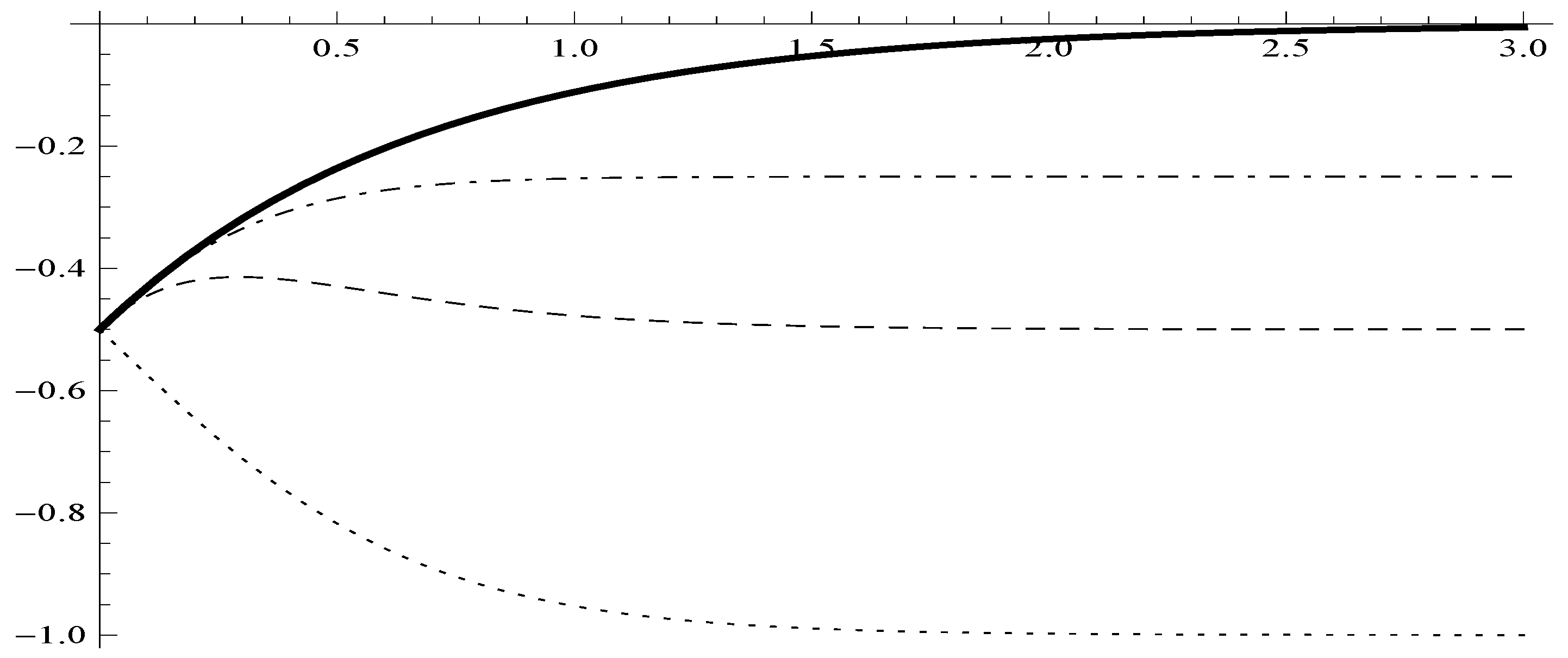
Example 1.

Suppose that the d.f. F is an exponential distribution with density

$$f\left(x\right)=3e^{-3x},x\ge 0$$

and the distribution of the inter-claim times is also an exponential distribution with density

$$k\left(t\right)=3e^{-3t},t\ge 0.$$

In this case, the associated moment generating functions are identical and given by

$$M_f\left(r\right)={\int }_0^{\infty }{e}^{Rx}f\left(x\right)dx=\frac{3}{3-r}={\int }_0^{\infty }{e}^{Rt}k\left(t\right)dt=M_k\left(r\right).$$

Assuming $c=2$, the solution of the equation $M_k(-cr)M_F\left(r\right)=1$ gives $R=1.5$, which is the adjustment coefficient, and then (4) gives $\varphi =0.5$. The probability of ruin for our example is $\psi \left(u\right)=0.5e^{-1.5u}$ and $h\left(u\right)=\psi \left(u\right)-e^{-Ru}=-0.5e^{-1.5u}$.

In Figure 1 we illustrate the actual value of the quantity $h\left(u\right)=\psi \left(u\right)-e^{-Ru}$ (solid line) and the performance of the bounds given by (19) (dashed line) and (20) (dot-dashed line), finally with dotted line we present the lower bound in (17) obtained by Psarrakos and Politis (2009a).

4.2. Bounds for the Ruin Probability under Aging Properties

For the rest of this section, let us assume that F is light-tailed, so that R exists.

Willmot et al. (2001) show if the d.f. F is NWUC (NBUC), then

$$\psi \left(u\right)\le (\ge )\varphi e^{-Ru}=:{\psi }_W\left(u\right).$$

(25)

In the next result, we improve the bound given in (25), under the assumption of NWU (NBU) ladder heights. NWU (NBU) class is a subclass of NWUC (NBUC).

Proposition 3.

If the d.f. F is NWU (NBU), then

$$\psi \left(u\right)\le (\ge )\varphi e^{-Ru}-g\left(u\right)-{\varphi }^{3}R{\int }_0^{\infty }{e}^{Ry}K(u,y)dy=:{\psi }_L\left(u\right),$$

(26)

with

$$K(u,y)={\int }_0^u\left(\overline{F}(u-t+y)-\overline{F}(u-t)\overline{F}\left(y\right)\right)dF\left(t\right).$$

(27)

Proof. 

By Psarrakos (2008), we know that if the labber height d.f. F is NWU (NBU) then a lower (upper) bound for the tail of the deficit $\overline{H}(u,y)$ is

$$\overline{H}(u,y)\ge (\le )\overline{F}\left(y\right)\psi \left(u\right)+\varphi \overline{F}(u+y)-\varphi \overline{F}\left(u\right)\overline{F}\left(y\right).$$

Inserting the above inequality into (6) and applying (1) we obtain

$$\begin{array}{c}\hfill \overline{H}(u,y)\ge (\le )\overline{F}\left(y\right)\psi \left(u\right)+\varphi \overline{F}(u+y)-\varphi \overline{F}\left(u\right)\overline{F}\left(y\right)+{\varphi }^{2}K(u,y).\end{array}$$

Inserting the above inequality into (16), we have

$$\begin{array}{cc}\hfill \frac{1}{R}\left(e^{-Ru}-\psi \left(u\right)\right)& ={\int }_0^{\infty }{e}^{Ry}\overline{H}(u,y)dy\hfill \\ & \ge (\le )\psi \left(u\right){\int }_0^{\infty }{e}^{Ry}\overline{F}\left(y\right)dy+\varphi {\int }_0^{\infty }{e}^{Ry}\left(\overline{F}(u+y)-\overline{F}\left(u\right)\overline{F}\left(y\right)\right)dy\hfill \\ & +{\varphi }^2{\int }_0^{\infty }{e}^{Ry}K(u,y)dy.\hfill \end{array}$$

Then by (5) and (15), we derive that

$$\begin{array}{cc}\hfill \frac{1}{R}\left(e^{-Ru}-\psi \left(u\right)\right)& \ge (\le )\frac{1-\varphi }{\varphi R}\psi \left(u\right)-\frac{\overline{F}\left(u\right)}{R}+\frac{\varphi \overline{F}\left(u\right)}{R}+\varphi e^{-Ru}{\int }_u^{\infty }{e}^{Rz}\overline{F}\left(z\right)dz\hfill \\ & +{\varphi }^2{\int }_0^{\infty }{e}^{Ry}K(u,y)dy.\hfill \end{array}$$

Solving by $\psi \left(u\right)$ we obtain the upper (lower) bound in (26). □

Another bound for the probability of ruin $\psi \left(u\right)$, under the assumption of NWUC (NBUC) ladder heights, is given by Psarrakos and Politis (2009a), namely:

$$\psi \left(u\right)\le (\ge )\varphi e^{-Ru}-{\varphi }^2{e}^{-Ru}{\int }_u^{\infty }{e}^{Rz}dF\left(z\right)+\varphi \overline{F}\left(u\right)=:{\psi }_P\left(u\right).$$

(28)

The bound given by (26) is a refinement of the bound (28) of Psarrakos and Politis (2009a). Indeed, the integral into (28) could be written as follows:

$$\begin{array}{cc}\hfill {\int }_u^{\infty }{e}^{Rz}dF\left(z\right)& =-{\left[e^{Rz}\overline{F}\left(z\right)\right]}_u^{\infty }+R{\int }_u^{\infty }{e}^{Rz}\overline{F}\left(z\right)dz\hfill \\ & =e^{Ru}\overline{F}\left(u\right)+R{\int }_u^{\infty }{e}^{Rz}\overline{F}\left(z\right)dz.\hfill \end{array}$$

Inserting the above into (28) and assuming NWU (NBU) ladder heights we have

$${\psi }_P\left(u\right)=\varphi e^{-Ru}-g\left(u\right)\ge (\le )\varphi e^{-Ru}-g\left(u\right)-{\varphi }^{3}R{\int }_0^{\infty }{e}^{Ry}K(u,y)dy.$$

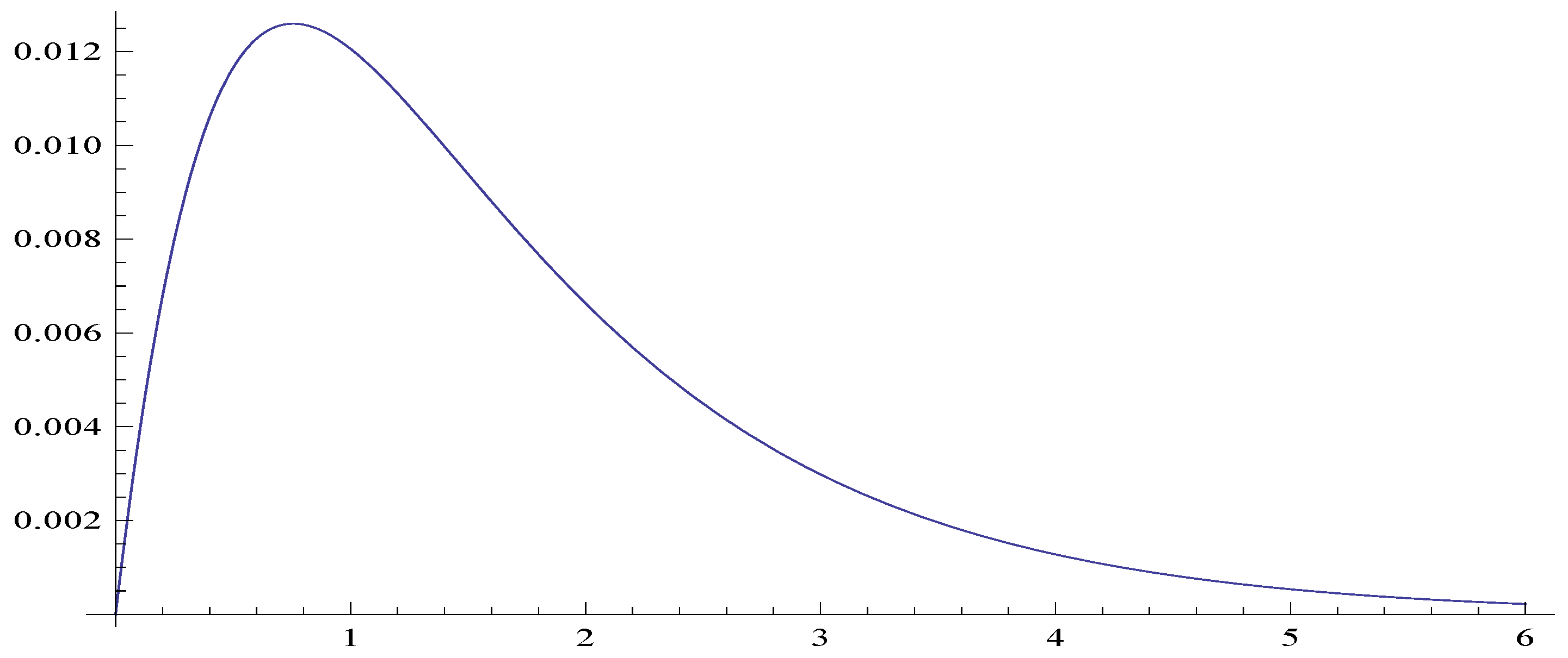
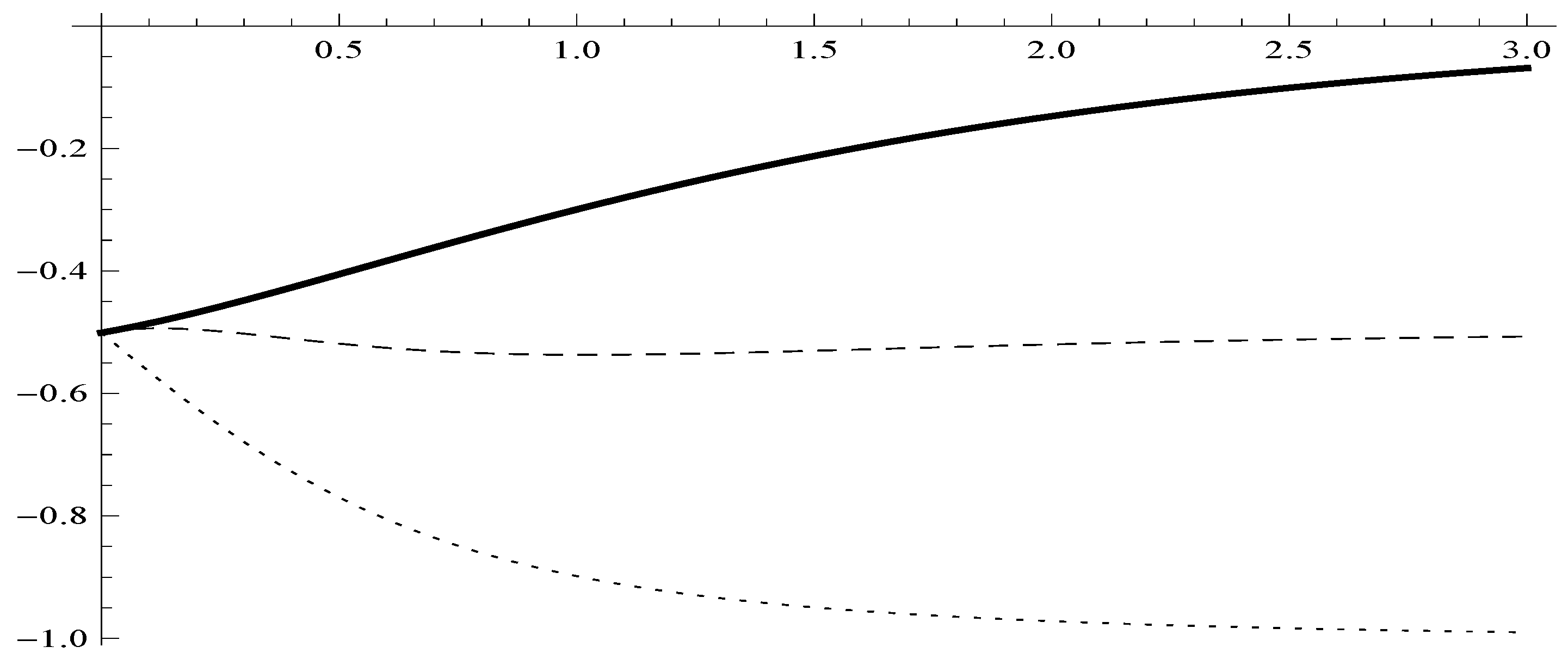
Example 2.

Suppose that the claim amount distribution is a mixture of exponential distributions with density

$$p\left(x\right)=\frac{1}{5}{e}^{-x}+\frac{12}{5}{e}^{-3x},$$

and the distribution of inter-claim times is an Erlang(2,2) distribution with density

$$k\left(t\right)=4t{e}^{-2t}.$$

We also assume $c=0.5$. In this case, the density of F is

$$f\left(x\right)=e^{-3x}\left(1.53088+0.489707e^{2x}\right),$$

while

$$R=0.128305,$$

$$\psi \left(u\right)=0.022519e^{-2.02621u}+0.890824e^{-0.128305u}.$$

Because of (26) and (28) we note that our proposed bounds perform better than the one given by Willmot et al. (2001); Psarrakos and Politis (2009a) only when $g\left(u\right)+{\varphi }^{3}R{\int }_0^{\infty }K(u,y)dy\ge 0$. In Lemma 4, we prove that the sign of the function $g\left(u\right)$ is linked with NWU (NBU) ladder heights. The mixture of exponential is always DFR (Willmot and Lin (2001, p. 10)), so we expect $g\left(u\right)\ge 0$ for $t\ge 0$. Also, from (27) we expect $K(u,y)\ge 0$ for $u,y\ge 0$.

In Figure 2 we depict the quantity $g\left(u\right)+{\varphi }^{3}R{\int }_0^{\infty }{e}^{Ry}K(u,y)dy$.

In the following

Table 1. Bounds for the ruin probability, $\psi \left(u\right)$, when $p\left(x\right)=e^{-x}/5+12e^{-3x}/5$ and $k\left(t\right)=4t{e}^{-2t}$.

	$\mathit{\psi }\left(\mathit{u}\right)$	${\mathit{\psi }}_{\mathit{P}}\left(\mathit{u}\right)$	${\mathit{\psi }}_{\mathit{L}}\left(\mathit{u}\right)$
$t=0$	0.913343	0.913343	0.913343
$t=0.25$	0.876272	0.887963	0.876517
$t=0.5$	0.843646	0.848396	0.844936
$t=0.75$	0.814023	0.821708	0.816955
$t=1$	0.786524	0.796565	0.791305
$t=1.5$	0.735945	0.748913	0.744057
$t=3$	0.606265	0.620477	0.618556
$t=5$	0.469011	0.480722	0.480331

we present the values of the ruin probability $\psi \left(u\right)$ and we compare it against ${\psi }_P\left(u\right)$ and ${\psi }_L\left(u\right)$.

Example 3.

Let us consider the case where the claim amount distribution is a mixture of exponential distributions with density

$$p\left(x\right)=\frac{1}{5}{e}^{-x}+\frac{12}{5}{e}^{-3x},$$

and the d.f. P of the inter-claim times is a Pareto distribution with density

$$k\left(t\right)=\frac{2}{{(1+t)}^3}.$$

We also assume $c=2$. In this case, we have

$$R=0.782835,$$

$$\varphi =0.499146$$

and

$$\psi \left(u\right)=0.228102e^{-1.91939u}+0.271044e^{-0.782835u}.$$

In Figure 3 we illustrate the actual value of the quantity $h\left(u\right)=\psi \left(u\right)-e^{-Ru}$ (solid line) and the performance of the bounds given by (19) (dashed line) and with the dotted line we present the lower bound in (17) obtained by Psarrakos and Politis (2009a).

In the following

Table 2. Bounds for the ruin probability, $\psi \left(u\right)$, when $p\left(x\right)=e^{-x}/5+12e^{-3x}/5$ and $k\left(t\right)=2/{(1+t)}^3$.

	$\mathit{\psi }\left(\mathit{u}\right)$	${\mathit{\psi }}_{\mathit{L}}\left(\mathit{u}\right)$	${\mathit{\psi }}_{\mathit{P}}\left(\mathit{u}\right)$
$t=0$	0.499146	0.499146	0.499146
$t=0.25$	0.364034	0.364711	0.370720
$t=0.5$	0.270618	0.273886	0.287773
$t=0.75$	0.204748	0.211491	0.229919
$t=1$	0.157358	0.167263	0.186931
$t=1.5$	0.096582	0.109944	0.126778
$t=3$	0.026608	0.035826	0.041236
$t=5$	0.0054247	0.008172	0.009088

we present the values of the ruin probability $\psi \left(u\right)$ and we compare it against ${\psi }_P\left(u\right)$ and ${\psi }_L\left(u\right)$.

In what follows, we present an upper bound for the probability of ruin $\psi \left(u\right)$ under the condition that the ladder height d.f. F is IFR.

Proposition 4.

If the d.f. F is IFR, then

$$\begin{array}{c}\hfill \psi \left(u\right)\le \frac{\varphi \overline{F}\left(u\right)}{\varphi \overline{F}\left(u\right)+(1-\varphi ){\overline{H}}_{\infty }\left(u\right)}{e}^{-Ru}.\end{array}$$

Proof. 

Let the ladder height d.f. F be IFR, then by Willmot (2002, Corollary 3.2) it holds that

$$\overline{H}(u,y)\ge \frac{\overline{F}(u+y)}{\overline{F}\left(u\right)}\psi \left(u\right).$$

Inserting the above into (16) we obtain

$$\begin{array}{c}\hfill e^{-Ru}-\psi \left(u\right)\ge \frac{\psi \left(u\right)}{\overline{F}\left(u\right)}R{\int }_0^{\infty }{e}^{Ry}\overline{F}(u+y)dy.\end{array}$$

Willmot (2002) proves that ${lim}_{t\to \infty }{\overline{H}}_u\left(y\right)={\overline{H}}_{\infty }\left(y\right)$, where

$${\overline{H}}_{\infty }\left(y\right)=\frac{\varphi R}{1-\varphi }{\int }_0^{\infty }{e}^{Rx}\overline{F}(x+y)dx.$$

(29)

In view of (29) the above inequality could be written as

$$\begin{array}{c}\hfill e^{-Ru}-\psi \left(u\right)\ge \frac{\psi \left(u\right)}{\overline{F}\left(u\right)}\frac{1-\varphi }{\varphi }{\overline{H}}_{\infty }\left(u\right).\end{array}$$

After some algebra and solving by $\psi \left(u\right)$ completes the proof. □

4.3. Bounds for the Probability of Ruin When R Does Not Exist

Chadjiconstantinidis and Xenos (2022) consider the random sum $S_{t,\varphi }=X_{t,1}+X_{t,2}+\dots +X_{t,N_{t,\varphi }}$ is a d.f., where for the counting random variable $N_{t,\varphi }$ it holds $\mathbb{P}(N_{t,\varphi }=m)=(1-\varphi F\left(t\right)){\left(\varphi F\left(t\right)\right)}^m$, and $X_t=X|X\le t$ is of d.f. with

$$F_t\left(u\right)=\left\{\begin{array}{cc}\hfill \frac{F\left(u\right)}{F\left(t\right)},& 0\le u\le t,\hfill \\ \hfill 1,& u>t.\hfill \end{array}\right.$$

By introducing the tail probability of the compound geometric sum $S_{t,\varphi }$ as follows:

$${\psi }_{t,\varphi }\left(u\right)=\mathbb{P}(S_{t,\varphi }>u)=\sum _{m=1}^{\infty }(1-\varphi F\left(t\right)){\left(\varphi F\left(t\right)\right)}^m{\overline{F}}_t^{\ast m}\left(u\right),0\le u\le t,$$

they gave the following formula for the probability of ruin:

$$\psi \left(u\right)=\frac{(1-\varphi ){\psi }_{t,\varphi }\left(u\right)+\varphi \overline{F}\left(t\right)}{1-\varphi +\varphi \overline{F}\left(t\right)},0\le u\le t.$$

(30)

For convenience, we define ${\varphi }_t=\varphi F\left(t\right)$. Chadjiconstantinidis and Xenos (2022) gave bounds for the probability of ruin under the assumption of NBU and DFR ladder heights, in more detail: If the d.f. F is DFR, then for any $t>0$ it holds

$$\psi \left(u\right)\le \frac{(1-\varphi ){\varphi }_t{e}^{-u{R}_{\varphi }\left(u\right)}+\varphi \overline{F}\left(t\right)}{1-\varphi +\varphi \overline{F}\left(t\right)},0\le u\le t$$

(31)

and for any $u>0$

$$\psi \left(u\right)\le \frac{(1-\varphi ){\varphi }_u{e}^{-u{R}_{\varphi }\left(u\right)}+\varphi \overline{F}\left(u\right)}{1-\varphi +\varphi \overline{F}\left(u\right)},$$

(32)

while for the case of NBU ladder heights, the above bounds hold with the reverse inequality.

In what follows, we improve those bounds, regarding the aging class, by employing the bounds we introduced in Section 4.2. Specifically, under the assumption that the d.f. F is NWU (NBU) it holds

$$\begin{array}{c}\hfill \psi \left(u\right)\le (\ge ){\psi }_W\left(u\right).\end{array}$$

If F is NWU (NBU), then $F_t$ is NWU (NBU) (see Chadjiconstantinidis and Xenos (2022)) and references therein). Applying the above inequality to ${\psi }_{t,\varphi }\left(u\right)$, and by replacing $\varphi$ and R with ${\varphi }_t=\varphi F\left(t\right)$, $R_{\varphi }\left(t\right)$ we, respectively, obtain:

$${\psi }_{t,\varphi }\left(u\right)\le (\ge ){\psi }_{t,\varphi ,W}\left(u\right),$$

(33)

where

$${\psi }_{t,\varphi ,W}\left(u\right)={\varphi }_t{e}^{-R_{\varphi }\left(t\right)u}.$$

(34)

In view of (34), (31) and (32) could be written as follows:

$$\psi \left(u\right)\le \frac{(1-\varphi ){\psi }_{t,\varphi ,W}\left(u\right)+\varphi \overline{F}\left(t\right)}{1-\varphi +\varphi \overline{F}\left(t\right)},0\le u\le t,$$

and for any $u>0$

$$\psi \left(u\right)\le \frac{(1-\varphi ){\psi }_{u,\varphi ,W}\left(u\right)+\varphi \overline{F}\left(u\right)}{1-\varphi +\varphi \overline{F}\left(u\right)}.$$

The above bounds are expressed in terms of the ladder height d.f. F. Although these are smoothly translated for the classical risk model in terms of the claim-size d.f. P, in the Sparre–Andersen model, the d.f. F of the ladder heights may not be available analytically. In this case bounds under assumptions regarding the claim-size d.f, P could be useful.

In the following result, we provide a refinement of the previously mentioned bound assuming that the claim-size distribution P is DFR.

Proposition 5.

If the d.f. P is DFR, then for any $t>0$ it holds

$$\psi \left(u\right)\le \frac{(1-\varphi ){\psi }_{t,\varphi ,W}\left(u\right)+\varphi \overline{F}\left(t\right)}{1-\varphi +\varphi \overline{F}\left(t\right)},0\le u\le t,$$

(35)

and for any $u>0$

$$\psi \left(u\right)\le \frac{(1-\varphi ){\psi }_{u,\varphi ,W}\left(u\right)+\varphi \overline{F}\left(u\right)}{1-\varphi +\varphi \overline{F}\left(u\right)}.$$

(36)

Proof. 

Szekli (1986, Lemma 3.2) proves that if the claim-size d.f. P is DFR, then the same holds for the ladder-height d.f. F, thus F is NWU. Inserting (33) into (30) we obtain (35). By letting $u=t$ in (35) we obtain (36). □

Chadjiconstantinidis and Xenos (2022) gave the following lower bound for the probability of ruin:

$$\psi \left(u\right)\ge \frac{1-\varphi }{1-{\varphi }^n}\sum _{m=1}^{n-1}{\varphi }^m{\overline{F}}^{\ast m}\left(u\right)+\left(1-\frac{1-\varphi }{1-{\varphi }^n}\sum _{m=1}^{n-1}{\varphi }^m{\overline{F}}^{\ast m}\left(u\right)\right){\overline{V}}_{\varphi ,n}\left(u\right),$$

where ${\overline{V}}_{\varphi ,n}\left(u\right)=1-V_{\varphi ,n}\left(u\right)$ (for $n=1,2,3,\dots$) is the tail probability of a compound geometric sum. In more detail, it holds:

$${\overline{V}}_{\varphi ,n}\left(u\right)=\sum _{m=1}^{\infty }(1-{\varphi }^n){\left({\varphi }^n\right)}^m{\left({\overline{F}}^{\ast n}\right)}^{\ast m}\left(u\right),u\ge 0,$$

(37)

and for $0\le u\le t$ they also prove that

$$\begin{array}{c}\hfill {\overline{V}}_{\varphi ,n}\left(u\right)=\frac{{\varphi }^n{\overline{F}}^{\ast n}\left(t\right)+(1-{\varphi }^n){\overline{V}}_{t,\varphi ,n}\left(u\right)}{1-{\varphi }^n+{\varphi }^n{\overline{F}}^{\ast n}\left(t\right)},\end{array}$$

where

$${\overline{V}}_{t,\varphi ,n}\left(u\right)=\sum _{m=1}^{\infty }\left(1-{\varphi }^n{F}^{\ast n}\left(t\right)\right){\varphi }^n{\left(F^{\ast n}\left(u\right)\right)}^{\ast m}.$$

Proposition 6.

If the d.f. F is $IFR$, then the ratio ${\overline{V}}_{\varphi ,n}\left(u\right)/{\overline{F}}^{\ast n}\left(u\right)$ is nondecreasing.

Proof. 

Dividing (37) by $F^{\ast n}$ we obtain:

$$\frac{{\overline{V}}_{\varphi ,n}\left(u\right)}{F^{\ast n}\left(u\right)}=\sum _{m=1}^{\infty }(1-{\varphi }^n){\left({\varphi }^n\right)}^m\frac{{\left({\overline{F}}^{\ast n}\right)}^{\ast m}\left(u\right)}{F^{\ast n}\left(u\right)},u\ge 0.$$

Barlow and Proschan (1996) prove that if F is IFR, then for $n=1,2,3,\dots$, $F^{\ast n}$ is also $IFR$. Also, Psarrakos and Politis (2009b) prove that if a d.f. F is $IFR$, then for any $m\ge 2$, the quantity ${\overline{F}}^{\ast m}\left(u\right)/\overline{F}\left(u\right)$ is nondecreasing. Replacing $\overline{F}\left(u\right)$ with ${\overline{F}}^{\ast n}\left(u\right)$ completes the proof. □

In view of (3) and (37) we note that ${\overline{V}}_{\varphi ,1}\left(u\right)=\psi \left(u\right)$.

4.4. Concluding Remarks

In this paper, we first introduce a renewal-type equation for the difference $\psi \left(u\right)-e^{-Ru}$, and using this result, we improve the Lundberg upper bound for the ruin probability by offering a general two-sided bound for the $\psi \left(u\right)$.

Next, using assumptions expressed in terms of the ladder height d.f. F, we derive bounds for the probability of ruin, refining the ones previously obtained by Willmot et al. (2001). These results are based on the assumption that the d.f F belongs to certain aging classes; however, in the Sparre–Andersen model, F may not be available analytically. For this reason, in Section 4.3, we offer bounds by making assumptions for the d.f P of the claim size.

Someone might wonder about specific conditions needed for the d.f. F to be DFR. Szekli (1986, Lemma 3.2), provided a sufficient condition for F to be DFR. Specifically, if the d.f. P is DFR, then F is DFR. In the classical risk model, a weaker assumption is that if P is IMRL, characterised by the condition that ${\int }_x^{\infty }\overline{P}\left(y\right)dy/\overline{P}\left(x\right)$ is nondecreasing for $x\ge 0$, then it follows that F is DFR (see, e.g., Willmot and Lin (2001)). In this case, the results of Chadjiconstantinidis and Xenos (2022) that assume DFR ladder heights, hold true by considering that the d.f. P is IMRL.

References

1. Asmussen, Soren, and Hansjorg Albrecher. 2010. Ruin Probabilities. Advanced Series on Statistical Science & Applied Probability. Singapore: World Scientific, vol. 14. [Google Scholar]
2. Barlow, Richard E., and Frank Proschan. 1996. Mathematical Theory of Reliability. Classics in Applied Mathematics. Philadelphia: Society for Industrial and Applied Mathematics (SIAM), vol. 17. [Google Scholar] [CrossRef]
3. Cai, Jun, and José Garrido. 1998. Aging properties and bounds for ruin probabilities and stop-loss premiums. Insurance: Mathematics and Economics 23: 33–43. [Google Scholar] [CrossRef]
4. Chadjiconstantinidis, Stathis, and Panos Xenos. 2022. Refinements of bounds for tails of compound distributions and ruin probabilities. Applied Mathematics and Computation 421: 126948. [Google Scholar] [CrossRef]
5. Dickson, David C. M. 1994. An upper bound for the probability of ultimate ruin. Scandinavian Actuarial Journal 1994: 131–38. [Google Scholar] [CrossRef]
6. Gerber, Hans U., Marc J. Goovaerts, and Rob Kaas. 1987. On the probability and severity of ruin. ASTIN Bulletin: The Journal of the IAA 17: 151–63. [Google Scholar] [CrossRef]
7. Labbé, Chantal, and Kristina P. Sendova. 2009. The expected discounted penalty function under a risk model with stochastic income. Applied Mathematics and Computation 215: 1852–67. [Google Scholar] [CrossRef]
8. Li, Shuanming, and Jose Garrido. 2005. On a general class of renewal risk process: Analysis of the Gerber-Shiu function. Advances in Applied Probability 37: 836–56. [Google Scholar] [CrossRef]
9. Psarrakos, Georgios. 2008. Tail bounds for the distribution of the deficit in the renewal risk model. Insurance: Mathematics and Economics 43: 197–202. [Google Scholar] [CrossRef]
10. Psarrakos, Georgios, and Konstadinos Politis. 2009a. A generalization of the Lundberg condition in the sparre andersen model and some applications. Stochastic Models 25: 90–109. [Google Scholar] [CrossRef]
11. Psarrakos, Georgios, and Konstadinos Politis. 2009b. Monotonicity properties and the deficit at ruin in the Sparre Andersen model. Scandinavian Actuarial Journal 2009: 104–18. [Google Scholar] [CrossRef]
12. Rolski, Tomasz, Hanspeter Schmidli, Volker Schmidt, and Jozef Teugels. 1999. Stochastic Processes for Insurance and Finance. Wiley Series in Probability and Statistics. Chichester: John Wiley & Sons, Ltd. [Google Scholar] [CrossRef]
13. Schmidli, Hanspeter. 2017. Risk Theory. Springer Actuarial. Cham: Springer. [Google Scholar] [CrossRef]
14. Szekli, Ryszard. 1986. On the concavity of the waiting-time distribution in some GI/G/1 queues. Journal of Applied Probability 23: 555–61. [Google Scholar] [CrossRef]
15. Temnov, Gregory. 2004. Risk process with random income. Journal of Mathematical Sciences 123: 3780–94. [Google Scholar] [CrossRef]
16. Temnov, Gregory. 2014. Risk models with stochastic premium and ruin probability estimation. Journal of Mathematical Sciences 196: 84–96. [Google Scholar] [CrossRef]
17. Willmot, Gordon E. 2002. Compound geometric residual lifetime distributions and the deficit at ruin. Insurance: Mathematics and Economics 30: 421–38. [Google Scholar] [CrossRef]
18. Willmot, Gordon E. 2007. On the discounted penalty function in the renewal risk model with general interclaim times. Insurance: Mathematics and Economics 41: 17–31. [Google Scholar] [CrossRef]
19. Willmot, Gordon E., and Jae-Kyung Woo. 2017. Surplus Analysis of Sparre Andersen Insurance Risk Processes. Springer Actuarial. Cham: Springer. [Google Scholar] [CrossRef]
20. Willmot, Gordon E., and X. Sheldon Lin. 2001. Lundberg Approximations for Compound Distributions with Insurance Applications. Lecture Notes in Statistics. New York: Springer, vol. 156. [Google Scholar] [CrossRef]
21. Willmot, Gordon E., Jun Cai, and X. Sheldon Lin. 2001. Lundberg inequalities for renewal equations. Advances in Applied Probability 33: 674–89. [Google Scholar] [CrossRef]
Figure 1. Bounds for the quantity h ( u ) when f ( x ) = 3 e 3 x and k ( t ) = 3 e 3 t .
Risks 12 00028 g001
Figure 2. The quantity g ( u ) + ϕ 3 R 0 e R y K ( u , y ) d y under NWU ladder heights.
Risks 12 00028 g002
Figure 3. Bounds for the quantity h ( u ) when p ( x ) = e x / 5 + 12 e 3 x / 5 and k ( t ) = 2 / ( 1 + t ) 3 .
Risks 12 00028 g003