
Maximum Pseudo-Likelihood Estimation of Copula Models and Moments of Order Statistics


School for Business and Society, University of York, York YO10 5DD, UK
Risks 2024, 12(1), 15; https://doi.org/10.3390/risks12010015
Submission received: 20 December 2023
/
Revised: 15 January 2024
/
Accepted: 16 January 2024
/
Published: 18 January 2024
(This article belongs to the Special Issue Interplay between Financial and Actuarial Mathematics II)
Abstract
:It has been shown that, despite being consistent and in some cases efficient, maximum pseudo-likelihood (MPL) estimation for copula models overestimates the level of dependence, especially for small samples with a low level of dependence. This is especially relevant in finance and insurance applications when data are scarce. We show that the canonical MPL method uses the mean of order statistics, and we propose to use the median or the mode instead. We show that the MPL estimators proposed are consistent and asymptotically normal. In a simulation study, we compare the finite sample performance of the proposed estimators with that of the original MPL and the inversion method estimators based on Kendall’s tau and Spearman’s rho. In our results, the modified MPL estimators, especially the one based on the mode of the order statistics, have a better finite sample performance both in terms of bias and mean square error. An application to general insurance data shows that the level of dependence estimated between different products can vary substantially with the estimation method used.
1. Introduction
Copula models are widely used in insurance and finance for pricing, hedging, and risk management, as well as in health sciences, hydrology, and other applied sciences; see e.g., Chen and Guo (2019); Czado (2019); Joe (2014); Kularatne et al. (2021); McNeil et al. (2015). Such wide applicability has triggered important contributions both in probabilistic and statistical aspects of copula models; see Durante and Sempi (2015); Joe (2014) and references therein. The estimation of copula model parameters from observed data appears, at first, to be a straightforward inference exercise. However, it has, in fact, significant pitfalls. The estimation of copula models without fully understanding the properties of the estimators can have undesirable consequences such as, among others, the overestimation of the dependence in the data; see the discussion in Fermanian and Scaillet (2005). One of the difficulties is that the distribution of the univariate margins is, in principle, unknown. Estimation procedures have been proposed to circumvent this problem, but no estimation procedure seems to be clearly the best. In fact, Kojadinovic and Yan (2010) show that the performance of commonly used estimation methods depends on the size of the sample and the strength of the dependence in the data. In finance, large samples of data are often available but the same does not happen in other applications where data are, by their nature, limited. This is the case, for instance, if the observations naturally occur at a low frequency or the population of interest is, by itself, small. Here, we propose new semiparametric estimators and show that the level of dependence obtained can differ substantially in a general insurance case where the data are available only quarterly.
Sklar’s representation theorem (Sklar 1959) characterizes a so-called copula model for a random vector with multivariate distribution H by a copula function, C, and univariate marginal cumulative distribution functions (cdfs) for , as
A copula is then a multivariate distribution with standard uniform univariate margins. If the univariate marginal cdfs are continuous, then the copula is unique. The versatility of copula models is apparent from Sklar’s representation theorem. By combining different distributions for the univariate margins with copula functions, a variety of models can be easily specified. Such flexibility can have a cost when it comes to the task of estimating the copula model from observed data.
Assuming that the univariate margins and copula all belong to absolutely continuous families of distributions, the obvious estimation method is maximum likelihood (ML). By default, the ML estimation of a model’s parameters is performed in one step. But, mainly due to numerical problems, which typically arise during the optimization of a likelihood function with several parameters and possibly multi-dimensional integrals, a two-step maximum likelihood estimation method has been introduced, the so-called inference functions for margins (IFM) from Joe and Xu (1996) and Joe (1997). The IFM method consists of estimating first the parameters for each univariate margin distribution independently, and then estimating the dependence parameters from the multivariate log-likelihood where the univariate margins parameter estimates are held fixed. Although the two-step IFM method can suffer from some loss of efficiency in cases of strong dependence, it still enjoys strong asymptotic efficiency as shown by Joe (2005). A further advantage of a two-step estimation method is that the estimation of the univariate margins parameters is not affected by a possible misspecification of the multivariate copula model. A fundamental challenge with the ML estimation, either the one or two-step procedure, is to ensure the correct choice of distributions for the univariate margins. This is especially relevant if we are particularly interested in modelling the dependence structure of the random vector. Through a simulation study, Fermanian and Scaillet (2005) find that misspecification of the margins may translate into a severe positive bias and high mean square errors in the estimation of the copula parameters leading to an overestimation of the degree of dependence in the data. An extensive simulation study from Kim et al. (2007) shows that the one-step ML and the IFM methods are indeed nonrobust against misspecification of the marginal distributions. Kim et al. (2007) also shows that, when the margins are unknown, in order to avoid the consequences of misspecification, it is better to use the maximum pseudo-likelihood (MPL) estimation procedure studied in Genest et al. (1995) and Shih and Louis (1995). Semiparametric estimation in copula models is indeed used widely even in nonstationary cases, for instance climate data, as is the case in Nasri et al. (2019).
For a random sample from distribution , the MPL is a semiparametric estimation procedure consisting of selecting the parameter that maximizes the log pseudo-likelihood function
where is the probability density function (pdf) of the copula family , and the univariate marginal distributions estimator is a rescaled empirical distribution function of the jth variable. Further asymptotic properties of the MPL estimator have been studied in Klaassen and Wellner (1997) and Genest and Werker (2002). The finite sample properties of the MPL estimator have been studied in Kojadinovic and Yan (2010) in a study where they compare the MPL estimator with the two method-of-moments (MM) estimators based on the inversion of Spearman’s rho and Kendall’s tau coefficients. The MM estimators have been studied by Genest (1987); Genest and Rivest (1993); Oakes (1982). Kojadinovic and Yan (2010) found that the MPL estimator performs better than the MM estimators in terms of mean squared error, except for small and weakly dependent vectors. Using the MM procedure as an alternative to MPL for small weakly dependent vectors is not the best solution, as we will demonstrate in this study. Instead, we propose to modify the canonical MPL estimator by using consistent nonparametric estimators of the univariate marginal distributions different from that used since Genest et al. (1995).
After deriving theoretically the consistency and asymptotic normality of the proposed MPL estimators, we study their small sample properties via a simulation study. We compare three alternative MPL estimators with the canonical MPL, and with the MM estimators based on the inversion of Kendall’s tau and Spearman’s rho. We find that changing the nonparametric estimator of the univariate margins indeed improves the finite sample performance of the MPL estimator, in terms of bias and mean squared error, while preserving its asymptotic properties. To confirm the large sample performance of the estimators we evaluate their relative efficiency via simulation.
Instead of proposing to use alternative nonparametric estimators of the univariate margins, another possibility would be to obtain a bias correction function for the canonical MPL estimator. Such a bias correction function would depend not only on the copula parameter and sample size, but also, importantly, on the specific copula itself. The approach that we propose to use here has the advantage of not depending on the specific copula. A bias reduction correction can also have the effect of increasing the variance of the estimator and possibly the mean square error, (see e.g., Søbye et al. 2021). That does not happen with the estimators we propose here.
Another possible approach is to estimate the multivariate model nonparametrically using empirical copulas, the asymptotic properties of which can be found in Genest and Segers (2010) and Segers et al. (2017). See also, e.g., Yang et al. (2020) on the nonparametric estimation of copula regression models. Naturally, empirical copula model estimation requires larger samples. Especially in applications where the size of the sample available is limited, there might be enough data to estimate the univariate marginal distribution functions nonparametrically but not enough data to estimate the empirical copula. That is one of the reasons why the semiparametric method from Genest et al. (1995) has become commonly used in applications.
Although we chose to compare the MPL estimators proposed here with the MM estimators, as in Kojadinovic and Yan (2010), other semiparametric estimators have been introduced in the literature. Tsukahara (2005) studied two semiparametric estimation procedures and concluded that these, overall, have a higher mean squared error when compared with the canonical MPL estimator. Chen et al. (2006) introduced and studied the properties of an MPL estimator where the unknown marginal density functions are approximated by linear combinations of finite-dimensional known basis functions with increasing complexity called sieves. They find that for weak dependence the sieve method performs comparably to the canonical MPL in finite samples. Given these results, comparing the proposed estimators with the canonical MPL and the MM estimators seems an appropriate choice.
In Section 2 of this article, we introduce the canonical MPL estimation procedure and its statistical properties. It is our starting point, as we benchmark the MPL estimators that we propose against the canonical MPL estimator. Section 3 motivates and proposes the new MPL estimators. Section 4 addresses their asymptotic properties. We show that the finite sample properties of the MPL estimators depend on the copula model in Section 5. Section 6 summarizes the MM estimators used in the simulation study. In Section 7 we report and discuss the results of the simulation study where we compare the small sample performance of the six estimators. We apply our results to a case of general insurance data in Section 8. Section 9 concludes the paper. Proofs and tables with simulation results are given in the Appendix A and Appendix B.
2. The Canonical MPL Estimator
Given a multivariate copula model with univariate marginal absolutely continuous distribution functions, the so-called canonical maximum pseudo-likelihood method consists of estimating univariate marginal distributions from the marginal empirical distributions, as a first step assuming that the univariate variables are independent, and then selecting the copula parameter that maximizes the log pseudo-likelihood function,
In the canonical MPL estimation, the so-called pseudo-observations are obtained from as
where is the empirical cumulative distribution function for , and denotes the indicator function of event A. The rescaling of the empirical distribution function by the factor in expression (2) is made to avoid computational problems on the boundary of . The use of the empirical distribution function to transform the margins to uniform can be traced back to Genest et al. (1995). The large sample properties of the canonical MPL estimator were studied by Genest et al. (1995) and Shih and Louis (1995), who showed that this estimator is consistent and asymptotically normal, and efficient at independence. Later, Genest and Werker (2002) argue that the latter is rather the exception than the rule and identify two cases of semiparametric efficiency. These are the independence and the normal copula, for which the result could already be found in Klaassen and Wellner (1997).
3. Alternative MPL Estimators
The semiparametric canonical MPL estimation procedure hinges on a nonparametric estimator of each marginal univariate distribution for . As introduced in the previous section, this nonparametric estimator is the rescaled empirical distribution function . Here, we motivate and propose the use of alternative nonparametric estimators for the univariate margins in the MPL estimation procedure.
In the implementation of the canonical MPL method, for each univariate margin , the pseudo-observations , defined in (2), are calculated as
where is the rank of among .
For clarification, MPL estimation presents no scalability problems. The estimators involve ranking the multivariate observations one margin at the time. Hence, it can be easily implemented for high dimensional data sets.
3.1. Pseudo-Observations and Moments of Order Statistics
To motivate the new estimators, first we show the relation between the pseudo-observations and order statistics. Assume that are n-independent and identically distributed (iid) univariate random variables. Arrange these in ascending order of magnitude as , and call the rth order statistic, for .
Proposition 1.
Consider a random sample from a univariate distribution with continuous cdf F and the corresponding transformed vector where for . If we define the function for , then each pseudo-observation , for , can be obtained as , where is the rank of among .
The proof of Proposition 1 can be found in the Appendix A. The conclusion is that the pseudo-observations in (3), proposed by Genest et al. (1995), can be obtained from the expected value of the order statistics defined as a function of the rank of the corresponding sample observations, i.e.,
where , for , and is the rank of within .
Note that, as we are assuming that the random variable X is continuous and its cdf F is an increasing function, we have that the rank of among is the same as the rank of among . We remark here that Clayton and Cuzick (1985) also used expected order statistics from unit exponential distributions in the estimation of the dependence parameter of a bivariate hazards model.
At this point, it is important to recall that our goal is to improve the performance of the canonical MPL which uses the pseudo-observations computed as in (4). With this objective in mind, we explore the properties of the pseudo-observations in (4) inherited from the fact that these are obtained from expected values of order statistics, and how this affects the performance of the canonical MPL estimator.
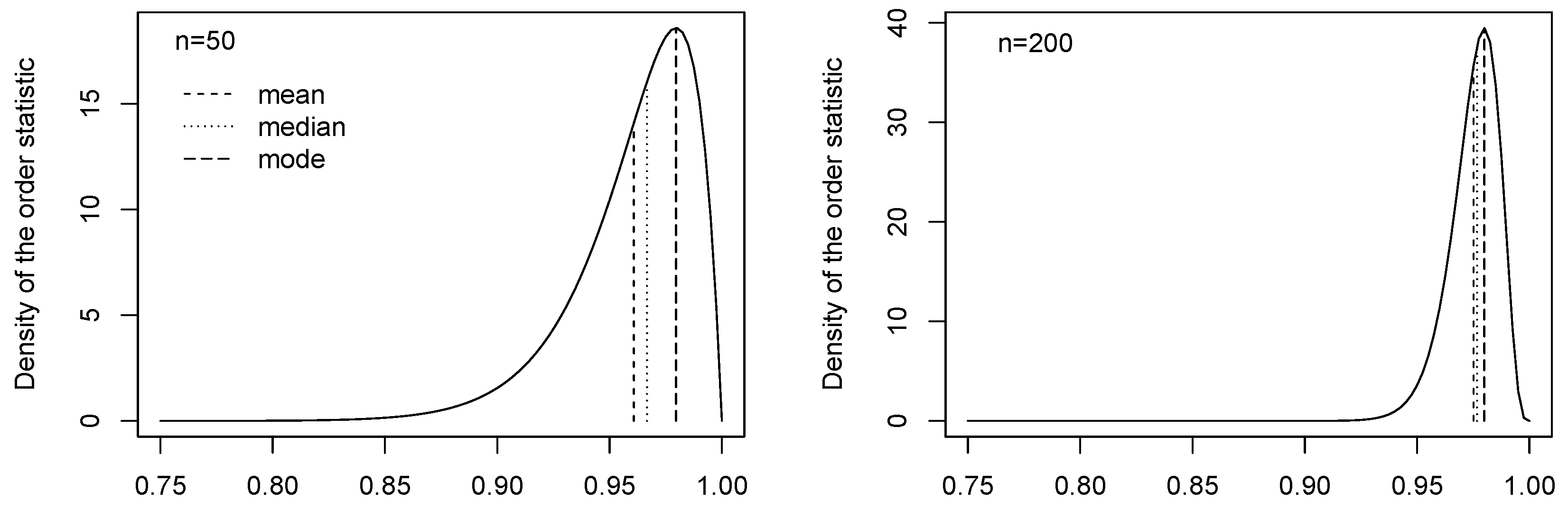
If the random variable X has cdf F, then the distribution of the order statistics is skewed (except for if n is even), especially when r is closer to 1 or n. Given that the expected value can be highly influenced by the skewness of the distribution, it is then possible that the properties of the pseudo-observations in (4) are affected by the skewness of and consequently also the canonical MPL estimator. Figure 1 displays the pdf of the order statistics and in , for samples of size and respectively. The strong skewness of the pdf implies that the mean is further away from the peak of the distribution than the median and, obviously, the mode. The pseudo-observations calculated using the mean of the order statistics might suffer from the skewness of the pdf. Hence, we propose to use the median or the mode of the order statistics, instead of the mean, to compute the pseudo-observations, and we study their effect on the performance of the new MPL estimators obtained from (1). From Figure 1 we can see that the skewness of the order statistics pdf is higher for smaller samples. We will see that, in fact, the smaller the sample, the larger the improvement of the performance of the estimator when using the median or the mode rather than the mean of the order statistics.
3.2. Pseudo-Observations and the Median of Order Statistics
We first propose to use the median of the rth order statistic as an alternative to using the mean of the order statistic. If the continuous random variable X has cdf F then is drawn from a standard uniform distribution and the median of the order statistic is
where is the regularised incomplete beta function. The computations can be made faster using the approximation (see Hyndman and Fan 1996; Kerman 2011) given by
Defining the function , the corresponding pseudo-observations for the estimation of the copula parameter via the pseudo-likelihood method are then
3.3. Pseudo-Observations and the Mode of Order Statistics
The second alternative we explore to compute the pseudo-observations is using the mode of the rth order statistic from a standard uniform distribution, which is given by
In this case, defining the function , the pseudo-observations are
We will refer to the copula parameter estimation procedure consisting of using the pseudo-observations given by (6) in the log pseudo-likelihood function as the mode MPL.
For the minimum and the maximum in each margin, i.e., for and (), it is not possible to use the mode of the corresponding order statistic as pseudo-observations in the pseudo log-likelihood function because these would be zero and one, respectively. In these cases, we use instead the mean of the order statistics and as in the canonical MPL because this is our benchmark estimator.
At this point we would like to remark the following. Instead of calculating the pseudo-observations as the mean, median or mode of the order statistics , we could consider using , or . If F is strictly monotonic then , which is one of the proposed estimators above. The pseudo-observations, calculated as or , depend on the distribution F. As we want to assume that F is unknown, we do not consider these alternatives.
3.4. Midpoint and Pseudo-Observations
In the canonical MPL estimator, the motivation to rescale the empirical distribution by multiplying it with is justified (starting with Genest et al. 1995) due to the need to keep the pseudo-observations away from the boundary of the interval . To that end, the adjustment to the empirical distribution function can rather be carried out using
Here, the additive factor ensures that the pseudo-observations are strictly in the interval . This approach, introduced by Hazen (1914), is popular with hydrologists and it is also used by Joe (2014) in the process of converting sample observations to normal scores. We include it in our study as an alternative to calculating the pseudo-observations, which are then given by
4. Large Sample Properties of the MPL Estimators
Before moving on to the small-sample performance simulation study, we consider the consistency and asymptotic normality of the different estimators. As already pointed out by other authors, (e.g., Genest et al. 1995; Kojadinovic and Yan 2010), using as pseudo-observations in the log pseudo-likelihood function in (1) corresponds to multiplying by the empirical distribution of the univariate jth variable. Each of the estimators of the univariate marginal distribution functions used above can be written as a function of the empirical distribution estimator for the corresponding variable. Given that the empirical distribution is a consistent estimator, as an immediate consequence of the strong law of large numbers, the consistency of the univariate cdf estimators used follows.
Genest et al. (1995) show the consistency and asymptotic normality of the canonical MPL estimator building on the work of Ruymgaart et al. (1972). In this section, we generalize their result for the median, mode, and midpoint MPL estimators proposed here. For simplicity of exposition, hereafter we consider bivariate distributions with copula , real parameter , and continuous univariate cdfs and , such that , . The results obtained can be generalised to the multivariate case.
The regularity conditions for the consistency and asymptotic normality of the MPL estimators are similar to those underlying the maximum likelihood estimator. Given a random sample from distribution , the MPL estimate takes the value that maximizes the log pseudo-likelihood function (1)
Let . The semiparametric estimate solves the equation
with denoting the partial derivative of l with respect to . To derive an expression for the semiparametric MPL estimator we follow Genest et al. (1995) and start by expanding (8) in a Taylor series. As a result, we obtain
where
and denotes the second derivative of l with respect to . Hence, a standardised version of is
whose large sample properties relate to those of multivariate rank statistics of the form
under the following assumptions.
Assumption 1.
is a continuous function from into such that
exists.
Assumption 2.
Define the function , on , let p and q be positive numbers satisfying and .
- (i)
- with M a positive constant, and ;
- (ii)
- with M a positive constant, and , and admits continuous partial derivatives on such that with and .
The limiting behaviour of the MPL estimators can then be summarised as follows.
Proposition 2.
Under assumptions 1 and 2, each of the median, mode and midpoint MPL estimators is consistent and is asymptotically normal with variance
where and
with denoting the indicator of A and .
The proof of Proposition 2 and necessary results are obtained in the Appendix A. The simulation study in Section 7 illustrates this result. For the cases of multidimensional dependence parameter or in a multivariate context, the previous results on the consistency and asymptotic normality of the modified MPL estimators can be extended as in Genest et al. (1995) following similar arguments.
5. Finite Sample Properties of the MPL Estimators
Consider the random sample of iid pairs from distribution . Let be the vector of ranks corresponding to , and the vector of ranks corresponding to . The mean square error of can be derived (at least approximated) from the moments of and and relation (9). Hence, we are interested in the properties of statistics and which are both of the form .
Let denote the inverse of in , the space of all permutations of . Define , where . We can then write the statistic in its dual form
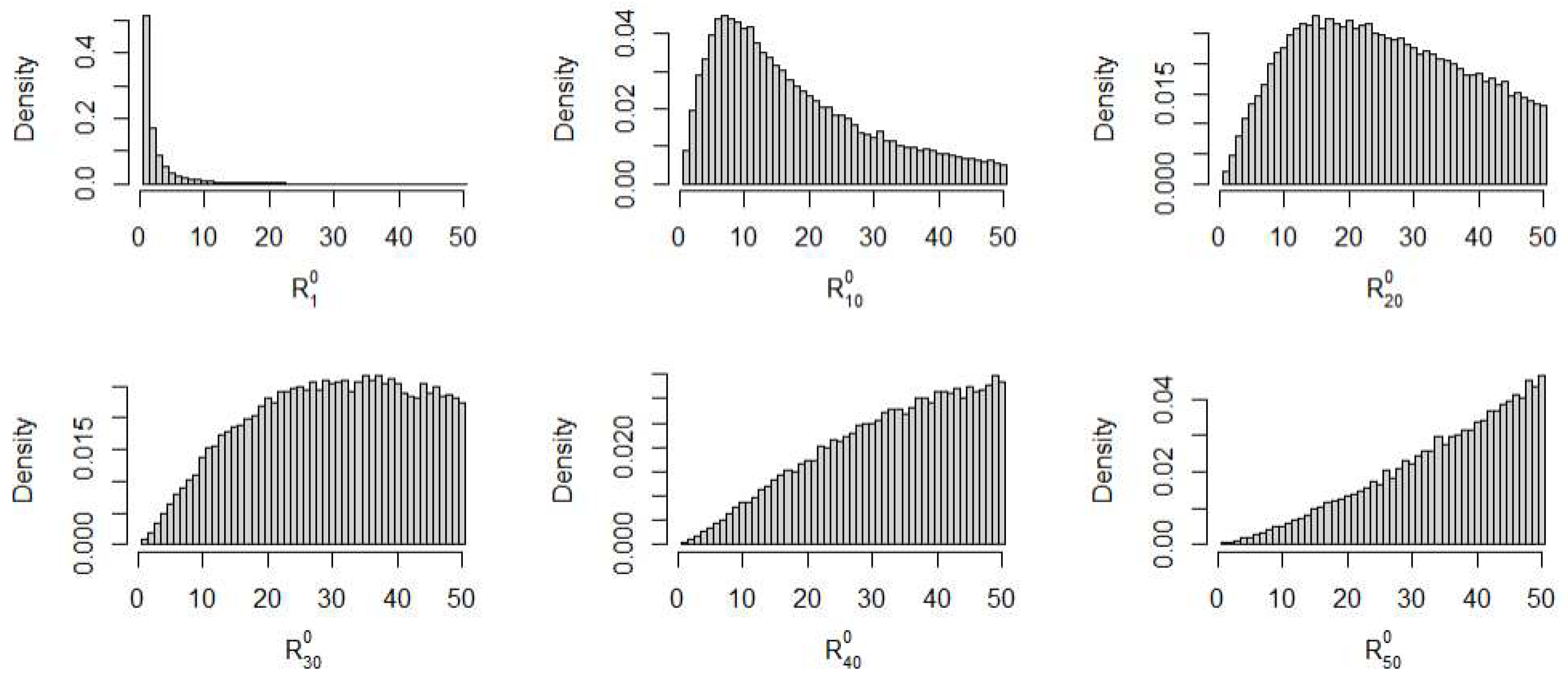
If and are independent then has a uniform distribution in and the derivation of its moments is straightforward (see e.g., Hájek 1969). Proposition 3 in the Appendix A shows how to obtain the moments of and given the distribution of . But if and are not independent then the distribution of , to the best of the author’s knowledge, is unknown. To give an idea of how different the distribution of the is from a uniform in the non independent case, we run a simulation from a Clayton copula with dependence parameter corresponding to a Kendall’s tau correlation of (see Joe 2014). We simulated 50,000 samples, each sample having pairs of observations from the Clayton copula. The histograms of the simulated observations of for are displayed in Figure 2. The histograms in Figure 2 show how the distribution of can be far from a uniform in the case of dependent samples. Given that the finite sample properties of the MPL estimators depend on the copula family via the unknown distribution of we proceed our investigation of the finite sample properties of the MPL estimators with a simulation study.
6. Method-of-Moments Estimators
In our simulation study, we also compare the performance of the four semiparametric MPL estimators with the method-of-moments (MM) estimators obtained from the relation between the copula parameter and the coefficients Kendall’s tau, , and Spearman’s rho, ; see Oakes (1982), Genest (1987), Genest and Rivest (1993). Copula parameter estimates obtained from these rank coefficients via the MM can be referred to as inversion-method estimates. The reason to include the two inversion-method estimators is first, because these perform better than the canonical MPL estimator for small weakly dependent samples, and second, to facilitate the comparison of our results with other related studies.
The MM estimation procedure is mostly used in the bivariate one-parameter copula model case, although it may be used in the multivariate and/or multiparameter cases, for instance, by imposing conditions on the dependence structure. In our simulation study we restrict ourselves to the one-parameter bivariate copulas case as explained in Section 7. Hence, consider the random sample from an absolutely continuous bivariate copula model , where belongs to an open subset of , and and are continuous cdfs. Inversion-method estimators rely on a consistent estimator of a copula moment. A consistent estimator of the copula moment Kendall’s tau is given by
Given the ranks corresponding to , where is the rank of among for , a consistent estimator of the bivariate copula moment Spearman’s rho is
The copula parameter estimate, , is then obtained by inversion from the relation between and or as or as , when the functions and are bijections. In those cases where there is no analytic expression for the relation between the copula parameter and or then a numerical approximation must be used. The consistency, asymptotic normality, and variance of and are well documented in the literature and we refrain from repeating it here, directing the reader to Kojadinovic and Yan (2010) and relevant references therein.
7. The Finite Sample Performance of the Estimators
In this section, we compare the performance of the semiparametric pseudo-likelihood estimator when calculating the pseudo-observations as in (4)–(7), and the MM Kendall’s tau and Spearman’s rho estimators. Recall that we refer to the MPL estimators for the copula model parameters corresponding to (4)–(7) as canonical MPL, median MPL, mode MPL, and midpoint MPL, respectively. To compare the performance of the six estimators, we perform a simulation study. The calculations are performed using R (R core Team 2020) and the package copula (Hofert et al. 2020).
Given their wide applicability to finance and insurance, we consider the copula families Clayton, Gumbel–Hougaard, Plackett, Normal, and Student-t. The Clayton family was first written in the form of a copula by Kimeldorf and Sampson (1975). Due to its joint lower tail dependence property, this family as been used to model the association between inter-event times, from epidemiology to insurance. The Gumbel (1960) copula can be used to model joint upper tail dependence, for instance, between large losses on financial assets or insurance claims. The bivariate Plackett (1965) family is radially symmetric and has been used as an alternative to the bivariate normal copula; see Nelsen (2006). The Normal and Student-t copulas are often used in classic finance and insurance multivariate models. Details on each of these copula families can be found, e.g., in Joe (2014). Without loss of generality, we consider the case of positive dependence in the simulation study.
We use six different levels of dependence corresponding to Kendall’s tau of 0.1, 0.2, 0.3, 0.4, 0.6, and 0.8, and four sample sizes of 50, 100, 200, and 400. These choices are also informed by the study of Kojadinovic and Yan (2010) to make it possible to benchmark some of our results against theirs. For each level of dependence and sample size, we simulate 5000 samples from all the copula families. Each sample is then used to estimate the copula parameter and standard error.
For clarification, we do not study the effect of the univariate marginal distributions because these play no role on the copula MPL estimation procedure. The pseudo-observations used in (1) to obtain the MPL estimators are adjusted ranks of each marginal observations and do not depend on the particular distribution of each margin. The set of ranks corresponding to an iid random sample from distribution F is a permutation T from the set of all possible permutations of . If the observations are independent, then the probability of obtaining permutation T is , independently of the distribution F, (see e.g., Hájek 1969).
7.1. Results
For each copula and degree of dependence considered, we present in Table A1, Table A2, Table A3 and Table A4 (in Appendix B) the results for sample sizes 50, 100, 200, and 400, respectively. In the tables, the different copula models are labelled as: C for the Clayton, G for the Gumbel–Hougaard, P for the Plackett, N for the Normal, and t for Student-t. For the six estimators, we report the percentage relative bias (PRB), the empirical standard deviation of the estimates (), the mean of the estimated standard errors (), and the empirical percentage coverage (PC) of the approximate 95% confidence interval for the dependence parameter calculated as . In the tables, we identify the results using a different subscript for each estimator. The notation for the canonical MPL is , for the median MPL is , for the mode MPL is , for the midpoint MPL is , for the MM Kendall’s tau inversion is , and for the MM Spearman’s rho inversion is .
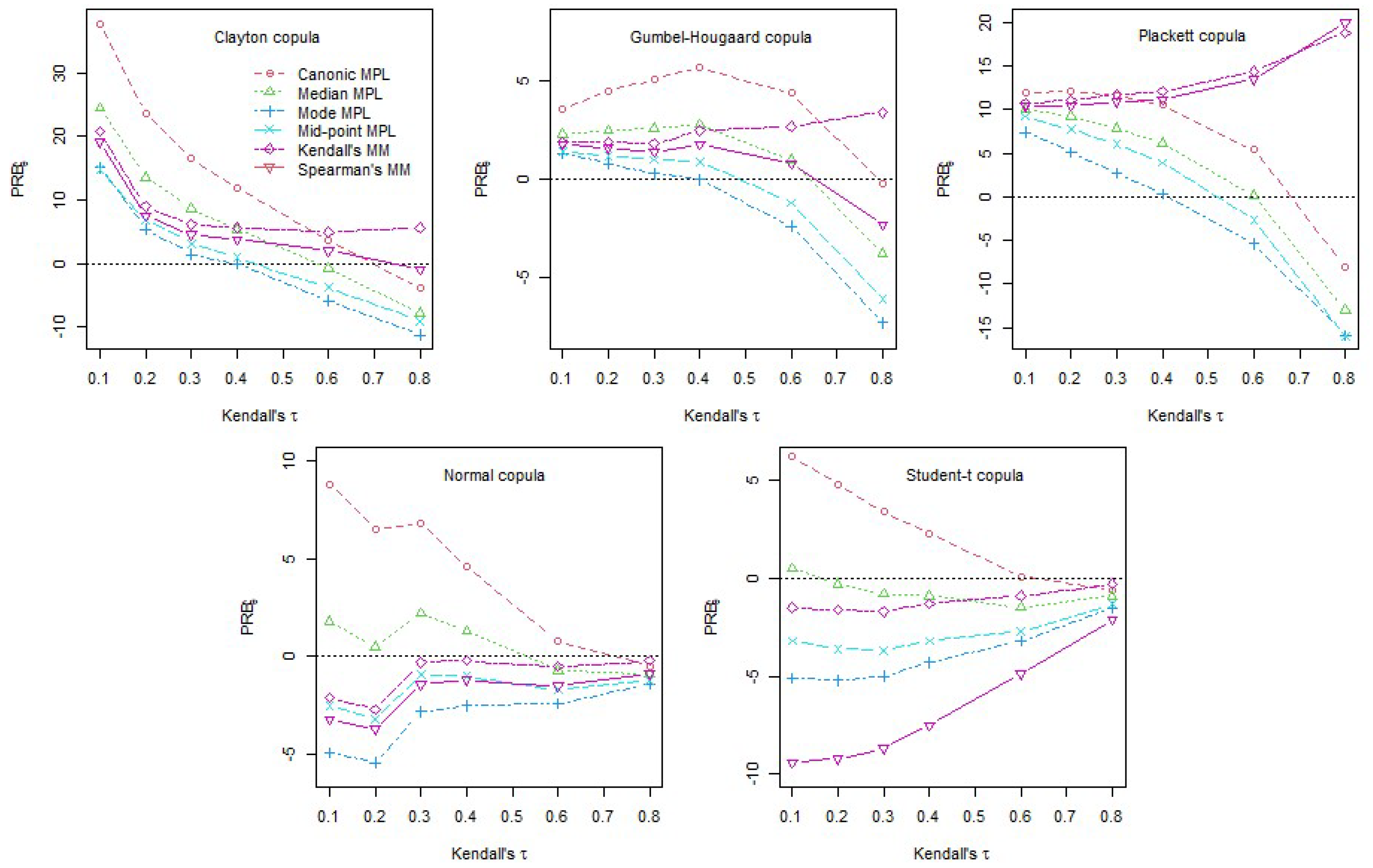
The results for the percentage relative bias can be visualised in Figure 3, where we plot the PRB for . As already observed by Kojadinovic and Yan (2010), the MM estimators have a smaller relative bias than the canonical MPL for small weakly dependent samples, except for the Student-t, where the Spearman’s inversion method performs quite poorly. However, the relative advantage of the MM estimators over the canonical MPL reduces when the sample size increases (see Table A2, Table A3 and Table A4 in Appendix B). For dependence levels the MM estimators can actually have a much larger PRB as it is the case for the Plackett copula. The newly considered median, mode and midpoint MPL estimators have smaller bias than the canonical MPL for weakly dependent samples () across all sample sizes. The mode and the midpoint MPL estimators have lower bias than the MM estimators for weakly dependent samples especially for smaller samples. The differences between the estimators in terms of bias reduce as the sample size increases. The median MPL performs remarkably well, in terms of bias, for the Normal and Student-t copulas across all levels of dependence.
The values for the empirical standard deviation of the estimates are very close to the mean of the estimated standard errors. This supports the assumptions underlying the estimator for the asymptotic variance. The empirical percentage coverage (PC) does not seem very different across the six estimators either. We can see that the PC tends to be larger than the 95% level for weaker dependence () and smaller than the 95% level for stronger dependence. From the results for the standard errors and percentage coverage obtained from the simulations, we find no evidence to contradict the asymptotic normality of the estimators. Overall, the results are consistent across the different copula families and sample sizes considered here.
Table A5 contains the estimated root mean square error (RMSE) for the canonical MPL estimator obtained for each sample size, copula, and level of dependence considered. The RMSE increases with the level of dependence, except for the Normal and Student-t, and decreases as the sample becomes larger. Hence, the higher RMSE for the canonical MPL estimator is observed for small strongly dependent samples and the lower RMSE is obtained from weakly dependent large samples. The increase in the RMSE with the level of dependence is supported by the fact that the estimated standard errors also increase with the strength of dependence, as shown in the PRB tables. For the Normal and Student-t copulas the estimated standard errors and RMSE of the canonical MPL decrease with the strength of the dependence and sample size.
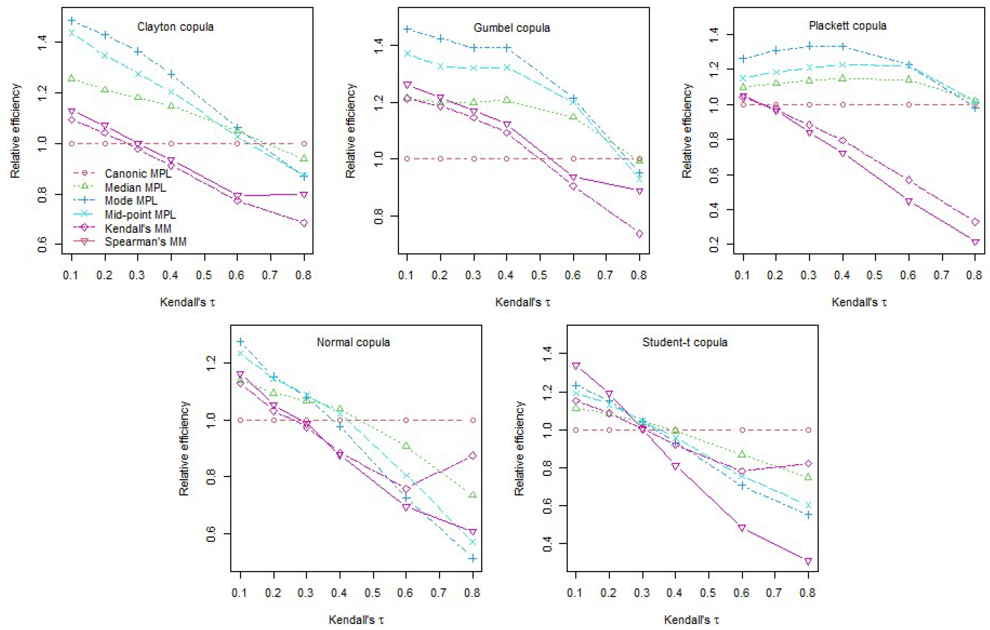
In Table A5, we also report the percentage relative efficiency (PRE) calculated as 100 times the estimated RMSE of the canonical MPL divided by the estimated RMSE of each of the other five estimators. We plot the PRE values in Figure 4 of the five estimators in relation to the canonical MPL for sample size . We observe that the MM Kendall’s tau- and Spearman’s rho-based estimators outperform the canonical MPL estimator for small weakly dependent samples but this advantage vanishes when the level of dependence becomes stronger or the sample size increases. These results are perfectly in line with the results from Kojadinovic and Yan (2010). The three semiparametric MPL estimators proposed here outperform, in terms of MSE, both MM estimators for all levels of dependence and sample size. Consequently, the three estimators introduced also outperform the canonical MPL for low dependence small samples. For stronger levels of dependence, , and samples larger than 100 the canonical MPL has the smallest MSE for the sample sizes considered. It is worth noting that, in the simulations, the proposed estimators substantially outperform the canonical MPL for weak dependence while for stronger dependence, the outperformance of the canonical MPL is modest. It is interesting that the MM estimators can have a quite poor performance in terms of MSE for stronger dependence in relation to the MPL estimators. Between the three MPL estimators introduced here, the mode MPL is overall the best for weakly dependent samples. This is particularly clear in Figure 4.
Finally, we estimate the asymptotic relative efficiency of the median MPL, mode MPL and midpoint MPL in relation to the canonical MPL estimator. The asymptotic percentage relative efficiency for each estimator is calculated as the estimated variance of the canonical MPL estimate, divided by the estimated variance of the MPL estimate given by the method being compared with, multiplied by 100. The estimates are obtained from a pseudo-randomly generated sample of size 100,000. The results, presented in Table A6, confirm that the three proposed MPL estimators and the canonical MPL estimator are asymptotically equally efficient.
8. Application to General Insurance Loss Ratios
In our application, we show the impact of using different MPL estimators while modelling the dependence between general insurance business classes, which is relevant for pricing, reserving and regulatory capital. We apply our results to loss ratios net of reinsurance from three insurance classes: houseowners/householders, domestic motor vehicles, and commercial motor vehicles. The data have been downloaded from the Australian Prudential Regulation Authority (APRA) (https://www.apra.gov.au/, accessed on 20 December 2023) general insurance statistics website. The historical loss ratios are available only from September 2010 until March 2023, comprising a sample of quarterly observations per insurance class.
Common factors underlying the risks covered under these three insurance classes, like weather conditions for instance, suggest the presence of dependence between the loss ratios. The Pearson’s linear correlation between houseowners/householders (house) and domestic motor vehicle (dom-motor) loss ratios is , between house and commercial motor vehicle (com-motor) is and between dom-motor and com-motor is . To select a copula model, we use the goodness-of-fit test from Genest et al. (2009) implemented in the R package copula. Although net of reinsurance, there might still be signs of upper joint tail dependence in the loss ratios. Indeed, a 180° rotated Clayton copula fitted to the loss ratios of house and dom-motor gives a p-value of , compared with from fitting a Gumbel copula, from a Student-t copula and from a normal copula. In panel A of Table 1, we list the estimates obtained from fitting a rotated Clayton model to house and dom-motor using the different MPL and MM estimators. For benchmarking, we also list the Kendall’s tau, , and upper tail dependence, , implied by the copula parameter estimates from the different methods. The mode MPL estimation produces the lowest copula parameter estimate and the lowest standard error, while the corresponding canonical MPL estimates are the largest among the MPL estimators. The MM estimators produce the largest copula estimates and standard errors. This agrees with the results we obtained for the finite sample performance of the estimators in Section 7.1. For a Clayton copula with , we observed that the mode MPL has the lowest PRB and standard error indicating that the mode MPL should give the least upward biased estimate of dependence. Comparing the results from the different estimators, note that the Kendall’s tau implied by the copula estimates ranges from to while the upper tail dependence ranges from to . Depending on the volume of earned premiums of these insurance classes on a particular insurance company, such variability will potentially have a significant financial impact on the calculation of reserves and regulatory capital of the firm.
For the case of house and com-motor loss ratios, with an even lower linear correlation of , the goodness-of-fit test from Genest et al. (2009) ranks first the 180° rotated Clayton copula model with a p-value of , followed by a Gumbel copula with , a normal copula with and a Student-t copula with a p-value. The results are consistent with the previous observations; see panel B in Table 1. The mode MPL produces the lowest overall estimate for the copula parameter and standard error, and the canonical MPL gives the highest estimates among the MPL estimators. The MM estimates are the highest across all the estimation methods. The implied Kendall’s tau varies now between and , while the upper tail dependence parameter ranges from to .
Finally, we consider the pair with the highest linear correlation among the named insurance classes reported in the APRA data: domestic motor vehicle and commercial motor vehicle. These two insurance classes have a sample linear correlation of between the corresponding loss ratios. In this case, the Gumbel copula model ranks first with a goodness-of-fit test p-value of . It is not surprising that a textbook three dimensional model, as a multivariate Gumbel or Clayton copulas for instance, does not have enough flexibility to accommodate real data as it is the case here. For the Gumbel copula model with parameter , Kendall’s tau is given by and the upper tail dependence parameter is ; see Joe (2014). The results from fitting a Gumbel copula model to com-motor and dom-motor, reported in panel C of Table 1, are coherent with those obtained for the previous two pairs of loss ratios. The mode MPL parameter estimate and standard error are the lowest across all the estimation methods, the canonical MPL has the largest estimates among the MPL estimators and the MM estimates are the largest overall. Nevertheless, the differences between the estimates are much smaller than in the previous two lower dependence cases, as we can see from the implied Kendall’s tau and upper tail coefficient estimates. The Kendall’s tau ranges between and and the upper tail coefficient varies from and .
From the three cases considered in this application, we observe that the variation of the estimates from the different MPL estimators increases as the dependence level decreases. The mode MPL has consistently the lowest parameter estimate and standard error. At a lower dependence level, the implied Kendall’s tau obtained by the MM estimators is almost double that obtained from the mode MPL. This study based on empirical data confirms what we would expect to observe according to the results we obtained in Section 7.1 for the finite sample performance of the estimators.
9. Conclusions
Kim et al. (2007) and Fermanian and Scaillet (2005) found that misspecification of the margins leads to non robust estimation of the dependence structure in a copula model with overestimation of the degree of dependence. Later, Kojadinovic and Yan (2010) found that overestimation of the degree of dependence can happen even when the unknown margins are estimated non-parametrically, especially for small weakly dependent samples.
We show here that the pseudo-observations used in the canonical MPL estimation method (Genest et al. 1995) can be seen as expected values of the order statistics and propose new estimators based on the corresponding median and mode instead. We derive the theoretical asymptotic properties of the new MPL estimators. Our simulation study shows that using the mode of the order statistics instead of the mean when calculating the pseudo-observations can reduce the overestimation of the level of dependence, outperforming the canonical MPL and the inversion methods’ Kendall’s tau and Spearman’s rho in terms of mean squared error for weakly dependent samples. For larger, strongly dependent samples, the canonical MPL still outperforms the proposed modified MPL estimators. Hence, within the conditions considered, our study shows that it is preferable to use the MPL estimator where the pseudo-observations are calculated as the mode of the order statistics rather than the mean.
In applications, data might naturally only be available in small samples. This is the case in our empirical study of quarterly general insurance loss ratios. Our application illustrates that the mode MPL estimator gives lower levels of dependence with smaller standard errors. The Kendall’s tau coefficient implied from the different estimators varies by up to more than , showing the importance of understanding well the performance of the different estimators.
Funding
This research received no external funding.
Data Availability Statement
The data used in this study is publicly available and can be found here: (https://www.apra.gov.au/, accessed on 20 December 2023).
Conflicts of Interest
The author declares no conflict of interest.
Appendix A. Proofs
Appendix A.1. Proof of Proposition 1
Proof.
Let , for , denote the cdf of the rth order statistic . It is well known, (see e.g., David and Nagaraja 2003), that
If we assume that is continuous, denoting the pdf of by we have that
where is the pdf of and , for and , is the beta function.
Given that the cdf of , for , is F, the random sample is drawn from a standard uniform distribution . Hence, the pdf of the rth order statistic has the expression
and belongs to the family of beta distributions. The mean of the rth order statistic for a random sample from a standard uniform distribution is then
Defining the function , for , gives the result. □
Appendix A.2. Proof of Proposition 2
Consider a continuous bivariate distribution with copula and marginals and such that .
Definition A1.
For a random sample , define the following rescaled versions of the empirical distribution for :
- (a)
- for ,
- (b)
- for ,
- (c)
- for and for , with and ,
- (d)
- for .
Let for denote any of the rescaled empirical distributions in Definition (A1). In order to proof Proposition 2 we first introduce two results concerning the asymptotic behaviour of statistics of the form
where is a continuous function from into such that
exists. Define the function , on , let p and q be positive numbers satisfying and .
Proposition A1.
If with M a positive constant, and , then almost surely.
First, note that all the rescaled empirical distribution functions (b), (c), and (d) in Definition (A1) are functions of the rescaled empirical distribution (a). The proof of Proposition (A1) can then be obtained following an argument similar to the one used by Genest et al. (1995) to prove their Proposition A1.
Proposition A2.
If with M a positive constant, and , and if J admits continuous partial derivatives on such that with and , then , with
The proof of Proposition (A2) can be obtained by using the rescaled empirical distributions in Definition (A1) (b), (c), and (d) in the proof of Theorem 2.1 of Ruymgaart et al. (1972).
Now to proof Proposition 2. we apply Proposition (A1) taking J equal to to obtain that almost sure. Then, taking J equal to in Proposition (A2), we obtain that with
giving the asymptotic results of Proposition 2.
Appendix A.3. Proposition 3
Proposition 3.
Consider the set of iid pairs of continuous random variables from distribution and the function f(r) from to . Then,
with and .
The expected value and variance of are obtained in a similar way by replacing and with and , respectively. The poof can be easily obtained from the definitions of expected value, variance, and covariance of a discrete random variable.
Appendix B. Simulation Results

Table A1.
Percentage relative bias (PRB), empirical standard deviation of the estimates (s), mean of the estimated standard errors (), and empirical percentage coverage (PC) of the approximate 95% confidence interval for the dependence parameter. Estimates based on 5000 pseudo-random samples of size .
| C | ||||||||||||||
| 0.1 | C | 0.22 | 37.8 | 0.232 | 0.240 | 97.4 | 24.5 | 0.213 | 0.224 | 98.2 | 15.1 | 0.200 | 0.211 | 98.9 |
| G | 1.11 | 3.6 | 0.125 | 0.134 | 98.1 | 2.3 | 0.117 | 0.128 | 98.6 | 1.3 | 0.108 | 0.122 | 99.0 | |
| P | 1.56 | 11.9 | 0.799 | 0.770 | 92.1 | 10.1 | 0.767 | 0.744 | 92.1 | 7.4 | 0.721 | 0.701 | 91.7 | |
| N | 0.16 | 8.8 | 0.157 | 0.155 | 91.3 | 1.8 | 0.147 | 0.149 | 92.6 | −4.9 | 0.139 | 0.142 | 93.7 | |
| t | 0.16 | 6.2 | 0.173 | 0.166 | 91.2 | 0.5 | 0.165 | 0.168 | 93.6 | −5.1 | 0.156 | 0.164 | 94.6 | |
| 0.2 | C | 0.50 | 23.7 | 0.298 | 0.289 | 94.6 | 13.6 | 0.284 | 0.273 | 94.4 | 5.4 | 0.267 | 0.267 | 93.6 |
| G | 1.25 | 4.5 | 0.164 | 0.164 | 94.6 | 2.5 | 0.156 | 0.159 | 93.5 | 0.8 | 0.145 | 0.155 | 92.9 | |
| P | 2.48 | 12.1 | 1.226 | 1.192 | 92.8 | 9.2 | 1.171 | 1.148 | 92.2 | 5.1 | 1.095 | 1.079 | 91.1 | |
| N | 0.31 | 6.5 | 0.142 | 0.138 | 90.0 | 0.5 | 0.137 | 0.136 | 91.7 | −5.4 | 0.132 | 0.133 | 93.1 | |
| t | 0.31 | 4.8 | 0.157 | 0.152 | 90.9 | −0.3 | 0.152 | 0.155 | 93.2 | −5.2 | 0.146 | 0.154 | 94.6 | |
| 0.3 | C | 0.86 | 16.5 | 0.367 | 0.361 | 94.7 | 8.6 | 0.355 | 0.343 | 93.3 | 1.4 | 0.337 | 0.346 | 92.4 |
| G | 1.43 | 5.1 | 0.205 | 0.203 | 94.3 | 2.6 | 0.195 | 0.197 | 93.2 | 0.3 | 0.184 | 0.196 | 92.9 | |
| P | 3.99 | 11.6 | 1.901 | 1.852 | 93.0 | 7.9 | 1.809 | 1.780 | 92.3 | 2.7 | 1.69 | 1.677 | 90.5 | |
| N | 0.45 | 6.8 | 0.121 | 0.115 | 88.3 | 2.2 | 0.121 | 0.116 | 91.0 | −2.8 | 0.12 | 0.119 | 93.1 | |
| t | 0.45 | 3.4 | 0.135 | 0.131 | 90.1 | −0.8 | 0.134 | 0.136 | 92.8 | −5 | 0.132 | 0.139 | 94.5 | |
| 0.4 | C | 1.33 | 11.8 | 0.463 | 0.464 | 94.5 | 5.3 | 0.451 | 0.442 | 93.0 | −1.0 | 0.433 | 0.457 | 91.9 |
| G | 1.67 | 5.7 | 0.249 | 0.252 | 94.7 | 2.8 | 0.238 | 0.246 | 93.8 | 0.0 | 0.226 | 0.248 | 93.4 | |
| P | 6.58 | 10.5 | 3.030 | 2.940 | 92.7 | 6.1 | 2.875 | 2.821 | 91.7 | 0.3 | 2.693 | 2.666 | 90.0 | |
| N | 0.59 | 4.6 | 0.092 | 0.092 | 89.0 | 1.3 | 0.094 | 0.095 | 91.6 | −2.5 | 0.096 | 0.101 | 94.7 | |
| t | 0.59 | 2.3 | 0.11 | 0.107 | 90.1 | −0.9 | 0.111 | 0.112 | 92.9 | −4.3 | 0.112 | 0.119 | 94.8 | |
| 0.6 | C | 3.00 | 3.7 | 0.796 | 0.854 | 94.5 | −0.8 | 0.784 | 0.840 | 92.0 | −5.9 | 0.759 | 0.879 | 92.1 |
| G | 2.50 | 4.4 | 0.413 | 0.424 | 94.9 | 1.0 | 0.398 | 0.415 | 93.5 | −2.4 | 0.383 | 0.427 | 92.8 | |
| P | 21.13 | 5.4 | 8.914 | 8.792 | 92.5 | 0.2 | 8.406 | 8.359 | 90.6 | −5.4 | 8.033 | 7.995 | 87.5 | |
| N | 0.81 | 0.8 | 0.051 | 0.051 | 90.9 | −0.7 | 0.054 | 0.054 | 93.6 | −2.4 | 0.057 | 0.06 | 95.9 | |
| t | 0.81 | 0.1 | 0.058 | 0.059 | 91.7 | −1.5 | 0.061 | 0.063 | 94.6 | −3.2 | 0.065 | 0.071 | 96.6 | |
| 0.8 | C | 8.00 | −3.9 | 1.803 | 2.354 | 94.5 | −7.9 | 1.799 | 2.366 | 93.4 | −11.3 | 1.741 | 2.517 | 93.3 |
| G | 5.00 | −0.2 | 0.871 | 1.014 | 95.0 | −3.8 | 0.853 | 0.993 | 92.0 | −7.3 | 0.814 | 1.063 | 92.2 | |
| P | 115 | −8.0 | 42.733 | 45.820 | 87.8 | −13 | 40.557 | 43.225 | 84.6 | −15.9 | 40.121 | 42.529 | 82.1 | |
| N | 0.95 | −0.5 | 0.015 | 0.02 | 98.5 | −0.9 | 0.017 | 0.021 | 98.9 | −1.4 | 0.018 | 0.025 | 99.3 | |
| t | 0.95 | −0.6 | 0.018 | 0.021 | 97.7 | −0.9 | 0.02 | 0.022 | 98.1 | −1.5 | 0.021 | 0.026 | 98.9 | |
| C | ||||||||||||||
| 0.1 | C | 0.22 | 14.9 | 0.203 | 0.213 | 98.5 | 20.8 | 0.231 | 0.246 | 99.0 | 19.2 | 0.228 | 0.242 | 99.2 |
| G | 1.11 | 1.4 | 0.111 | 0.126 | 98.7 | 1.9 | 0.117 | 0.126 | 98.8 | 1.8 | 0.115 | 0.120 | 98.8 | |
| P | 1.56 | 9.2 | 0.751 | 0.730 | 91.9 | 10.7 | 0.787 | 0.756 | 91.8 | 10.4 | 0.784 | 0.736 | 91.6 | |
| N | 0.16 | −2.5 | 0.141 | 0.145 | 93.3 | −2.1 | 0.148 | 0.147 | 93.2 | −3.2 | 0.146 | 0.142 | 92.8 | |
| t | 0.16 | −3.2 | 0.159 | 0.171 | 94.6 | −1.5 | 0.162 | 0.160 | 93.4 | −9.4 | 0.149 | 0.159 | 95.1 | |
| 0.2 | C | 0.50 | 6.8 | 0.274 | 0.261 | 93.5 | 9.0 | 0.311 | 0.306 | 94.0 | 7.5 | 0.308 | 0.308 | 94.3 |
| G | 1.25 | 1.2 | 0.150 | 0.158 | 92.3 | 1.9 | 0.158 | 0.156 | 94.2 | 1.6 | 0.156 | 0.149 | 93.4 | |
| P | 2.48 | 7.8 | 1.144 | 1.125 | 91.8 | 11.1 | 1.247 | 1.200 | 91.9 | 10.5 | 1.257 | 1.179 | 91.7 | |
| N | 0.31 | −3.2 | 0.134 | 0.134 | 92.6 | −2.7 | 0.141 | 0.137 | 92.8 | −3.7 | 0.139 | 0.134 | 92.5 | |
| t | 0.31 | −3.6 | 0.148 | 0.159 | 94.5 | −1.6 | 0.151 | 0.150 | 93.3 | −9.2 | 0.142 | 0.149 | 94.9 | |
| 0.3 | C | 0.86 | 3.1 | 0.348 | 0.329 | 91.8 | 6.2 | 0.394 | 0.382 | 93.7 | 4.6 | 0.392 | 0.394 | 94.0 |
| G | 1.43 | 1.0 | 0.189 | 0.196 | 92.1 | 1.8 | 0.201 | 0.196 | 94.3 | 1.4 | 0.200 | 0.186 | 92.4 | |
| P | 3.99 | 6.0 | 1.762 | 1.743 | 91.7 | 11.7 | 2.028 | 1.931 | 92.4 | 10.9 | 2.088 | 1.931 | 91.4 | |
| N | 0.45 | −0.9 | 0.119 | 0.117 | 91.9 | −0.3 | 0.127 | 0.121 | 92.4 | −1.4 | 0.126 | 0.119 | 92.3 | |
| t | 0.45 | −3.7 | 0.132 | 0.139 | 94.3 | −1.7 | 0.136 | 0.134 | 93.1 | −8.7 | 0.130 | 0.134 | 94.7 | |
| 0.4 | C | 1.33 | 0.9 | 0.446 | 0.427 | 90.5 | 5.6 | 0.507 | 0.485 | 93.5 | 3.8 | 0.504 | 0.515 | 94.2 |
| G | 1.67 | 0.9 | 0.231 | 0.245 | 92.7 | 2.5 | 0.251 | 0.250 | 94.6 | 1.8 | 0.249 | 0.233 | 93.1 | |
| P | 6.58 | 3.9 | 2.793 | 2.758 | 91.3 | 12.1 | 3.394 | 3.214 | 92.1 | 11.2 | 3.577 | 3.272 | 90.9 | |
| N | 0.59 | −1.0 | 0.094 | 0.097 | 92.9 | −0.2 | 0.102 | 0.102 | 92.8 | −1.2 | 0.102 | 0.101 | 93.0 | |
| t | 0.59 | −3.2 | 0.111 | 0.117 | 94.4 | −1.3 | 0.115 | 0.114 | 92.8 | −7.5 | 0.115 | 0.114 | 94.2 | |
| 0.6 | C | 3.00 | −3.8 | 0.785 | 0.839 | 89.6 | 4.9 | 0.901 | 0.848 | 93.0 | 2.0 | 0.900 | 1.002 | 95.0 |
| G | 2.50 | −1.2 | 0.389 | 0.420 | 92.2 | 2.7 | 0.444 | 0.436 | 95.0 | 0.8 | 0.441 | 0.395 | 91.4 | |
| P | 21.13 | −2.7 | 8.114 | 8.132 | 89.3 | 14.4 | 11.534 | 10.745 | 92.9 | 13.5 | 13.100 | 11.758 | 90.0 | |
| N | 0.81 | −1.7 | 0.055 | 0.056 | 94.7 | −0.5 | 0.059 | 0.058 | 92.4 | −1.5 | 0.059 | 0.059 | 93.9 | |
| t | 0.81 | −2.7 | 0.064 | 0.066 | 95.6 | −0.9 | 0.066 | 0.065 | 92.4 | −4.9 | 0.073 | 0.065 | 94.0 | |
| 0.8 | C | 8.00 | −9.1 | 1.814 | 2.372 | 92.5 | 5.6 | 2.165 | 2.002 | 93.2 | −1.0 | 2.046 | 3.380 | 96.6 |
| G | 5.00 | −6.1 | 0.848 | 1.00 | 90.1 | 3.4 | 0.999 | 1.067 | 96.1 | −2.3 | 0.916 | 1.112 | 92.2 | |
| P | 115 | −16.0 | 39.213 | 41.761 | 82.3 | 18.8 | 72.894 | 66.481 | 93.1 | 20.0 | 90.796 | 104.475 | 89.2 | |
| N | 0.95 | −1.2 | 0.018 | 0.023 | 98.7 | −0.2 | 0.017 | 0.019 | 94.8 | −0.9 | 0.019 | 0.026 | 99.8 | |
| t | 0.95 | −1.3 | 0.021 | 0.024 | 98.2 | −0.3 | 0.021 | 0.021 | 93.6 | −2.1 | 0.028 | 0.021 | 92.8 |
Table A2.
Percentage relative bias (PRB), empirical standard deviation of the estimates (s), mean of the estimated standard errors (), and empirical percentage coverage (PC) of the approximate 95% confidence interval for the dependence parameter. Estimates based on 5000 pseudo-random samples of size .
| C | ||||||||||||||
| 0.1 | C | 0.22 | 22.2 | 0.160 | 0.155 | 95.8 | 14.2 | 0.151 | 0.148 | 96.3 | 7.1 | 0.143 | 0.142 | 96.2 |
| G | 1.11 | 2.1 | 0.085 | 0.087 | 97.2 | 1.3 | 0.082 | 0.085 | 97.6 | 0.5 | 0.077 | 0.082 | 97.5 | |
| P | 1.56 | 6.5 | 0.520 | 0.507 | 94.0 | 5.8 | 0.509 | 0.498 | 93.9 | 4.5 | 0.492 | 0.482 | 93.6 | |
| N | 0.16 | 4.5 | 0.104 | 0.105 | 94.1 | 0.4 | 0.100 | 0.102 | 94.5 | −4.4 | 0.096 | 0.098 | 94.7 | |
| t | 0.16 | 5.2 | 0.118 | 0.116 | 92.9 | 1.6 | 0.114 | 0.117 | 94.3 | −2.7 | 0.11 | 0.116 | 95.1 | |
| 0.2 | C | 0.50 | 13.8 | 0.196 | 0.190 | 94.1 | 7.7 | 0.190 | 0.183 | 94.2 | 1.5 | 0.181 | 0.182 | 93.8 |
| G | 1.25 | 2.7 | 0.110 | 0.109 | 94.3 | 1.5 | 0.107 | 0.107 | 94.1 | 0.3 | 0.102 | 0.106 | 93.8 | |
| P | 2.48 | 6.6 | 0.804 | 0.786 | 94.1 | 5.3 | 0.786 | 0.771 | 93.8 | 3.1 | 0.757 | 0.744 | 93.1 | |
| N | 0.31 | 2.4 | 0.094 | 0.095 | 93.1 | −1.1 | 0.092 | 0.093 | 94.1 | −5.3 | 0.090 | 0.092 | 94.5 | |
| t | 0.31 | 3.6 | 0.108 | 0.107 | 92.7 | 0.4 | 0.106 | 0.108 | 93.9 | −3.4 | 0.103 | 0.109 | 95.2 | |
| 0.3 | C | 0.86 | 9.2 | 0.243 | 0.240 | 94.8 | 4.3 | 0.238 | 0.232 | 93.4 | −0.9 | 0.230 | 0.237 | 92.8 |
| G | 1.43 | 3.1 | 0.138 | 0.135 | 94.0 | 1.6 | 0.134 | 0.133 | 93.7 | 0.02 | 0.128 | 0.134 | 93.6 | |
| P | 3.99 | 6.2 | 1.243 | 1.222 | 94.2 | 4.5 | 1.213 | 1.198 | 93.8 | 1.7 | 1.166 | 1.157 | 92.8 | |
| N | 0.45 | 4.1 | 0.085 | 0.079 | 90.8 | 1.4 | 0.085 | 0.079 | 92.3 | −2.1 | 0.084 | 0.082 | 94.1 | |
| t | 0.45 | 2.5 | 0.094 | 0.092 | 92.1 | −0.1 | 0.094 | 0.095 | 93.7 | −3.3 | 0.093 | 0.097 | 95.0 | |
| 0.4 | C | 1.33 | 6.5 | 0.309 | 0.310 | 94.2 | 2.6 | 0.305 | 0.299 | 92.9 | −1.9 | 0.298 | 0.312 | 92.5 |
| G | 1.67 | 3.2 | 0.170 | 0.169 | 94.3 | 1.6 | 0.166 | 0.166 | 94.2 | −0.3 | 0.160 | 0.168 | 94.0 | |
| P | 6.58 | 5.5 | 1.971 | 1.941 | 94.1 | 3.4 | 1.920 | 1.901 | 93.5 | 0.2 | 1.845 | 1.838 | 92.3 | |
| N | 0.59 | 2.6 | 0.065 | 0.065 | 91.3 | 0.6 | 0.065 | 0.066 | 93.3 | −1.9 | 0.066 | 0.069 | 95.2 | |
| t | 0.59 | 1.7 | 0.077 | 0.076 | 91.5 | −0.3 | 0.078 | 0.078 | 93.5 | −2.8 | 0.079 | 0.082 | 95.2 | |
| 0.6 | C | 3.00 | 1.8 | 0.528 | 0.561 | 94.7 | −0.8 | 0.524 | 0.556 | 93.1 | −4.3 | 0.514 | 0.595 | 93.3 |
| G | 2.50 | 2.6 | 0.282 | 0.283 | 94.5 | 0.5 | 0.276 | 0.280 | 93.9 | −1.8 | 0.268 | 0.288 | 93.3 | |
| P | 21.1 | 2.6 | 5.797 | 5.799 | 93.7 | 0.1 | 5.618 | 5.654 | 92.8 | −3.6 | 5.414 | 5.473 | 91.0 | |
| N | 0.81 | 0.5 | 0.036 | 0.035 | 91.8 | −0.4 | 0.037 | 0.036 | 93.7 | −1.6 | 0.039 | 0.039 | 95.6 | |
| t | 0.81 | 0.1 | 0.041 | 0.041 | 92.7 | −0.8 | 0.043 | 0.043 | 94.1 | −2 | 0.045 | 0.046 | 96.0 | |
| 0.8 | C | 8.00 | −3.4 | 1.198 | 1.533 | 95.6 | −5.4 | 1.199 | 1.587 | 94.9 | −8.1 | 1.176 | 1.742 | 95.1 |
| G | 5.00 | −0.3 | 0.591 | 0.658 | 95.2 | −2.5 | 0.583 | 0.660 | 93.9 | −5.1 | 0.569 | 0.710 | 93.7 | |
| P | 115 | −6.0 | 27.836 | 29.825 | 90.5 | −8.9 | 26.916 | 28.828 | 88.5 | −11.7 | 26.386 | 28.279 | 85.9 | |
| N | 0.95 | −0.3 | 0.010 | 0.012 | 98.0 | −0.5 | 0.011 | 0.013 | 98.2 | −0.8 | 0.011 | 0.015 | 98.6 | |
| t | 0.81 | 0.1 | 0.041 | 0.041 | 92.7 | −0.8 | 0.043 | 0.043 | 94.1 | −2.0 | 0.045 | 0.046 | 95.9 | |
| C | ||||||||||||||
| 0.1 | C | 0.22 | 8.5 | 0.146 | 0.143 | 95.6 | 12.8 | 0.167 | 0.171 | 97.9 | 11.9 | 0.165 | 0.169 | 98.2 |
| G | 1.11 | 0.7 | 0.079 | 0.084 | 97.5 | 1.1 | 0.085 | 0.086 | 98.2 | 1.1 | 0.083 | 0.083 | 98.6 | |
| P | 1.56 | 5.4 | 0.504 | 0.493 | 93.8 | 5.7 | 0.513 | 0.503 | 93.8 | 5.8 | 0.515 | 0.498 | 93.6 | |
| N | 0.16 | −2.2 | 0.097 | 0.099 | 94.6 | −2.1 | 0.103 | 0.103 | 94.3 | −2.5 | 0.102 | 0.101 | 94.2 | |
| t | 0.16 | −0.7 | 0.112 | 0.119 | 95 | 0.4 | 0.113 | 0.113 | 93.6 | −7.3 | 0.105 | 0.113 | 95.6 | |
| 0.2 | C | 0.50 | 3.5 | 0.186 | 0.178 | 93.1 | 5.5 | 0.212 | 0.212 | 94.9 | 4.6 | 0.211 | 0.213 | 94.9 |
| G | 1.25 | 0.8 | 0.104 | 0.107 | 93.6 | 1.1 | 0.110 | 0.107 | 94.5 | 0.9 | 0.110 | 0.105 | 93.7 | |
| P | 2.48 | 4.7 | 0.777 | 0.763 | 93.5 | 5.9 | 0.816 | 0.800 | 93.5 | 5.7 | 0.825 | 0.797 | 93.6 | |
| N | 0.31 | −3.4 | 0.091 | 0.093 | 94.3 | −2.8 | 0.096 | 0.097 | 94.3 | −3.3 | 0.096 | 0.095 | 94.2 | |
| t | 0.31 | −1.6 | 0.104 | 0.11 | 94.7 | −0.4 | 0.106 | 0.106 | 93.8 | −7.7 | 0.100 | 0.106 | 95.5 | |
| 0.3 | C | 0.86 | 1.0 | 0.235 | 0.225 | 92.2 | 3.5 | 0.264 | 0.265 | 94.4 | 2.6 | 0.266 | 0.271 | 94.9 |
| G | 1.43 | 0.7 | 0.131 | 0.133 | 93.3 | 1.2 | 0.138 | 0.134 | 94.3 | 1.0 | 0.140 | 0.133 | 92.8 | |
| P | 3.99 | 3.7 | 1.198 | 1.185 | 93.5 | 6.0 | 1.302 | 1.279 | 94.4 | 5.7 | 1.348 | 1.305 | 93.7 | |
| N | 0.45 | −0.4 | 0.084 | 0.081 | 93.1 | 0.0 | 0.088 | 0.085 | 93.5 | −0.6 | 0.089 | 0.084 | 93.3 | |
| t | 0.45 | −1.8 | 0.093 | 0.097 | 94.5 | −0.5 | 0.095 | 0.094 | 93.4 | −7.2 | 0.092 | 0.094 | 94.9 | |
| 0.4 | C | 1.33 | −0.0 | 0.303 | 0.290 | 91.2 | 3.4 | 0.341 | 0.337 | 94.8 | 2.4 | 0.343 | 0.351 | 95.5 |
| G | 1.67 | 0.5 | 0.163 | 0.166 | 93.7 | 1.4 | 0.173 | 0.170 | 94.5 | 1.1 | 0.174 | 0.165 | 94.3 | |
| P | 6.58 | 2.4 | 1.894 | 1.881 | 93.2 | 6.2 | 2.166 | 2.128 | 94.1 | 5.8 | 2.290 | 2.214 | 93.6 | |
| N | 0.59 | −0.8 | 0.066 | 0.067 | 94.0 | −0.2 | 0.071 | 0.071 | 94.1 | −0.8 | 0.072 | 0.071 | 94.3 | |
| t | 0.59 | −1.7 | 0.078 | 0.08 | 94.6 | −0.4 | 0.08 | 0.079 | 92.9 | −6.2 | 0.081 | 0.079 | 94.4 | |
| 0.6 | C | 3.00 | −2.6 | 0.525 | 0.559 | 91.8 | 2.9 | 0.596 | 0.588 | 94.1 | 1.5 | 0.617 | 0.657 | 95.3 |
| G | 2.50 | −0.7 | 0.273 | 0.283 | 93.3 | 1.6 | 0.295 | 0.293 | 94.5 | 0.7 | 0.301 | 0.283 | 92.4 | |
| P | 21.1 | −1.3 | 5.520 | 5.577 | 92.3 | 7.1 | 7.168 | 7.028 | 94.4 | 6.9 | 8.341 | 7.85 | 93.0 | |
| N | 0.81 | −0.9 | 0.038 | 0.037 | 94.4 | −0.3 | 0.04 | 0.039 | 93.3 | −0.8 | 0.042 | 0.04 | 94.3 | |
| t | 0.81 | −1.5 | 0.044 | 0.044 | 94.9 | −0.3 | 0.045 | 0.044 | 92.8 | −4.1 | 0.051 | 0.044 | 91.9 | |
| 0.8 | C | 8.00 | −6.7 | 1.209 | 1.626 | 94.6 | 2.7 | 1.417 | 1.361 | 93.8 | −0.3 | 1.451 | 1.871 | 97.2 |
| G | 5.00 | −3.9 | 0.581 | 0.682 | 93.3 | 1.8 | 0.652 | 0.679 | 95.7 | −1.0 | 0.655 | 0.642 | 93.5 | |
| P | 115 | −10.6 | 26.36 | 28.271 | 86.7 | 8.4 | 42.741 | 41.63 | 94.4 | 10.9 | 59.905 | 54.611 | 92.6 | |
| N | 0.95 | −0.7 | 0.011 | 0.014 | 98.3 | −0.1 | 0.011 | 0.012 | 95.1 | −0.5 | 0.012 | 0.014 | 98.3 | |
| t | 0.81 | −1.5 | 0.044 | 0.044 | 94.9 | −0.3 | 0.045 | 0.044 | 92.8 | −4.1 | 0.051 | 0.044 | 91.9 |
Table A3.
Percentage relative bias (PRB), empirical standard deviation of the estimates (s), mean of the estimated standard errors (), and empirical percentage coverage (PC) of the approximate 95% confidence interval for the dependence parameter. Estimates based on 5000 pseudo-random samples of size .
| 0.1 | C | 0.22 | 9.2 | 0.106 | 0.103 | 94.1 | 4.5 | 0.102 | 0.100 | 94.0 | −0.4 | 0.098 | 0.097 | 93.5 |
| G | 1.11 | 1.0 | 0.056 | 0.058 | 95.1 | 0.5 | 0.055 | 0.058 | 94.8 | 0.02 | 0.053 | 0.056 | 94.5 | |
| P | 1.56 | 2.1 | 0.345 | 0.340 | 94.0 | 1.8 | 0.342 | 0.337 | 94.0 | 1.2 | 0.336 | 0.332 | 93.8 | |
| N | 0.16 | 3.0 | 0.072 | 0.072 | 94.7 | 0.6 | 0.07 | 0.071 | 94.9 | −2.6 | 0.068 | 0.069 | 94.8 | |
| t | 0.16 | 2.6 | 0.081 | 0.081 | 94.3 | 0.5 | 0.08 | 0.082 | 94.9 | −2.4 | 0.077 | 0.082 | 95.8 | |
| 0.2 | C | 0.50 | 6.6 | 0.133 | 0.129 | 94.2 | 2.9 | 0.131 | 0.126 | 93.9 | −1.2 | 0.127 | 0.126 | 93.4 |
| G | 1.25 | 1.3 | 0.072 | 0.074 | 95.4 | 0.6 | 0.071 | 0.073 | 95.2 | −0.1 | 0.069 | 0.073 | 94.8 | |
| P | 2.48 | 2.1 | 0.533 | 0.528 | 94.1 | 1.5 | 0.528 | 0.523 | 94.0 | 0.4 | 0.517 | 0.513 | 93.5 | |
| N | 0.31 | 1.3 | 0.064 | 0.066 | 95.2 | −0.8 | 0.063 | 0.065 | 95.2 | −3.5 | 0.062 | 0.065 | 95.1 | |
| t | 0.31 | 2.0 | 0.075 | 0.075 | 93.9 | 0.1 | 0.074 | 0.076 | 94.7 | −2.4 | 0.073 | 0.077 | 95.6 | |
| 0.3 | C | 0.86 | 4.1 | 0.169 | 0.165 | 94.0 | 1.2 | 0.167 | 0.161 | 92.9 | −2.3 | 0.164 | 0.164 | 92.6 |
| G | 1.43 | 1.5 | 0.090 | 0.092 | 95.2 | 0.7 | 0.088 | 0.092 | 95.2 | −0.3 | 0.086 | 0.092 | 94.9 | |
| P | 3.99 | 1.9 | 0.828 | 0.822 | 94.6 | 1.1 | 0.818 | 0.814 | 94.2 | −0.3 | 0.801 | 0.799 | 93.5 | |
| N | 0.45 | 2.8 | 0.06 | 0.056 | 92.2 | 1.2 | 0.06 | 0.056 | 93.1 | −0.9 | 0.06 | 0.057 | 93.8 | |
| t | 0.45 | 1.4 | 0.065 | 0.065 | 93.6 | −0.2 | 0.065 | 0.067 | 94.7 | −2.3 | 0.065 | 0.068 | 95.8 | |
| 0.4 | C | 1.33 | 2.8 | 0.216 | 0.212 | 93.8 | 0.5 | 0.214 | 0.207 | 92.8 | −2.5 | 0.212 | 0.214 | 92.4 |
| G | 1.67 | 1.5 | 0.113 | 0.115 | 95.3 | 0.5 | 0.111 | 0.114 | 95.0 | −0.7 | 0.109 | 0.115 | 95.0 | |
| P | 6.58 | 1.6 | 1.313 | 1.308 | 94.8 | 0.6 | 1.296 | 1.294 | 94.3 | −1.1 | 1.267 | 1.27 | 93.6 | |
| N | 0.59 | 1.4 | 0.046 | 0.046 | 93.5 | 0.2 | 0.046 | 0.046 | 94.5 | −1.5 | 0.046 | 0.048 | 95.4 | |
| t | 0.59 | 0.9 | 0.054 | 0.054 | 93.1 | −0.3 | 0.054 | 0.055 | 94.6 | −1.9 | 0.055 | 0.057 | 95.7 | |
| 0.6 | C | 3.00 | 0.0 | 0.373 | 0.379 | 94.4 | −1.5 | 0.372 | 0.375 | 92.8 | −3.7 | 0.368 | 0.401 | 93.2 |
| G | 2.50 | 1.1 | 0.188 | 0.193 | 95.0 | −0.01 | 0.186 | 0.192 | 94.5 | −1.5 | 0.183 | 0.196 | 94.3 | |
| P | 21.13 | 0.2 | 3.898 | 3.916 | 94.4 | −1.0 | 3.837 | 3.866 | 93.8 | −3.1 | 3.745 | 3.79 | 92.5 | |
| N | 0.81 | 0.4 | 0.026 | 0.025 | 92.7 | −0.2 | 0.026 | 0.025 | 93.5 | −0.9 | 0.027 | 0.026 | 94.3 | |
| t | 0.81 | 0.1 | 0.029 | 0.029 | 93.2 | −0.5 | 0.03 | 0.029 | 94.3 | −1.2 | 0.031 | 0.031 | 95.8 | |
| 0.8 | C | 8.00 | −2.9 | 0.845 | 1.001 | 95.2 | −4.1 | 0.845 | 1.048 | 94.9 | −5.8 | 0.835 | 1.175 | 95.2 |
| G | 5.00 | −0.4 | 0.402 | 0.438 | 95.6 | −1.7 | 0.399 | 0.443 | 95.0 | −3.4 | 0.393 | 0.476 | 94.1 | |
| P | 115 | −4.3 | 19.454 | 20.246 | 92.2 | −5.9 | 19.091 | 19.878 | 90.9 | −7.9 | 18.728 | 19.531 | 89.0 | |
| N | 0.95 | −0.1 | 0.007 | 0.008 | 96.9 | −0.3 | 0.007 | 0.008 | 97.2 | −0.5 | 0.008 | 0.009 | 97.7 | |
| t | 0.95 | −0.2 | 0.008 | 0.009 | 96.2 | −0.3 | 0.008 | 0.009 | 96.6 | −0.5 | 0.009 | 0.01 | 97.4 | |
| 0.1 | C | 0.22 | 1.2 | 0.100 | 0.097 | 93.7 | 3.6 | 0.119 | 0.118 | 94.3 | 3.2 | 0.118 | 0.117 | 94.6 |
| G | 1.11 | 0.2 | 0.054 | 0.058 | 94.6 | 0.5 | 0.059 | 0.059 | 95.0 | 0.5 | 0.058 | 0.058 | 95.4 | |
| P | 1.56 | 1.6 | 0.340 | 0.336 | 93.9 | 1.6 | 0.344 | 0.337 | 94.0 | 1.9 | 0.348 | 0.339 | 93.7 | |
| N | 0.16 | −0.9 | 0.069 | 0.07 | 95.0 | −0.8 | 0.072 | 0.073 | 94.9 | −0.9 | 0.072 | 0.072 | 94.9 | |
| t | 0.16 | −0.9 | 0.079 | 0.083 | 95.5 | −0.2 | 0.079 | 0.08 | 94.8 | −7.8 | 0.073 | 0.08 | 96.6 | |
| 0.2 | C | 0.50 | 0.4 | 0.129 | 0.124 | 93.1 | 1.8 | 0.148 | 0.147 | 94.4 | 1.3 | 0.148 | 0.147 | 94.5 |
| G | 1.25 | 0.2 | 0.070 | 0.073 | 94.9 | 0.5 | 0.073 | 0.074 | 95.2 | 0.3 | 0.074 | 0.073 | 94.9 | |
| P | 2.48 | 1.2 | 0.525 | 0.520 | 94.0 | 1.9 | 0.552 | 0.542 | 93.4 | 2.0 | 0.559 | 0.543 | 93.8 | |
| N | 0.31 | −2.0 | 0.062 | 0.065 | 95.1 | −1.7 | 0.066 | 0.068 | 95.2 | −2.0 | 0.066 | 0.067 | 95.2 | |
| t | 0.31 | −1.1 | 0.073 | 0.077 | 95.2 | −0.3 | 0.074 | 0.075 | 94.5 | −7.6 | 0.07 | 0.075 | 96.1 | |
| 0.3 | C | 0.86 | −0.7 | 0.166 | 0.157 | 92.0 | 0.8 | 0.185 | 0.184 | 94.5 | 0.4 | 0.188 | 0.188 | 94.6 |
| G | 1.43 | 0.2 | 0.088 | 0.091 | 94.6 | 0.5 | 0.091 | 0.093 | 95.3 | 0.5 | 0.094 | 0.094 | 94.7 | |
| P | 3.99 | 0.7 | 0.813 | 0.810 | 93.9 | 1.9 | 0.876 | 0.860 | 94.3 | 2.1 | 0.917 | 0.889 | 94.0 | |
| N | 0.45 | 0.2 | 0.06 | 0.056 | 93.4 | 0.3 | 0.062 | 0.06 | 94.0 | 0.0 | 0.062 | 0.06 | 94.0 | |
| t | 0.45 | −1.2 | 0.065 | 0.067 | 95.4 | −0.4 | 0.066 | 0.067 | 94.4 | −7 | 0.064 | 0.067 | 95.1 | |
| 0.4 | C | 1.33 | −1.0 | 0.214 | 0.202 | 91.6 | 1.0 | 0.240 | 0.234 | 94.1 | 0.6 | 0.245 | 0.242 | 94.5 |
| G | 1.67 | −0.04 | 0.110 | 0.114 | 95.0 | 0.5 | 0.116 | 0.117 | 95.4 | 0.5 | 0.117 | 0.116 | 95.1 | |
| P | 6.58 | 0.1 | 1.287 | 1.287 | 94.1 | 2.0 | 1.465 | 1.434 | 94.3 | 2.2 | 1.567 | 1.512 | 93.9 | |
| N | 0.59 | −0.6 | 0.046 | 0.047 | 94.9 | −0.2 | 0.049 | 0.05 | 95.1 | −0.5 | 0.05 | 0.05 | 94.9 | |
| t | 0.59 | −1.1 | 0.055 | 0.056 | 95.2 | −0.3 | 0.056 | 0.056 | 94.5 | −5.9 | 0.056 | 0.056 | 93.4 | |
| 0.6 | C | 3.00 | −2.5 | 0.37 | 0.37 | 91.9 | 0.7 | 0.418 | 0.409 | 93.9 | 0.1 | 0.440 | 0.446 | 94.3 |
| G | 2.50 | −0.7 | 0.185 | 0.194 | 94.4 | 0.6 | 0.198 | 0.201 | 95.4 | 0.2 | 0.206 | 0.202 | 94.7 | |
| P | 21.13 | −1.7 | 3.805 | 3.841 | 93.4 | 2.6 | 4.842 | 4.723 | 94.6 | 2.7 | 5.701 | 5.397 | 93.1 | |
| N | 0.81 | −0.5 | 0.027 | 0.025 | 93.9 | −0.1 | 0.028 | 0.027 | 94.1 | −0.3 | 0.029 | 0.028 | 94.2 | |
| t | 0.81 | −0.9 | 0.03 | 0.03 | 94.7 | −0.2 | 0.031 | 0.031 | 93.9 | −3.8 | 0.036 | 0.031 | 86.3 | |
| 0.8 | C | 8.00 | −4.8 | 0.850 | 1.089 | 95.2 | 0.8 | 0.975 | 0.943 | 94.0 | −0.6 | 1.044 | 1.162 | 95.6 |
| G | 5.00 | −2.6 | 0.398 | 0.461 | 94.8 | 0.8 | 0.441 | 0.453 | 95.9 | −0.4 | 0.466 | 0.445 | 92.7 | |
| P | 115 | −6.8 | 18.877 | 19.680 | 90.2 | 3.1 | 28.605 | 27.771 | 94.0 | 5.2 | 41.698 | 36.979 | 91.2 | |
| N | 0.95 | −0.4 | 0.007 | 0.009 | 97.1 | 0.0 | 0.008 | 0.008 | 95.3 | −0.2 | 0.008 | 0.009 | 96.6 | |
| t | 0.95 | −0.4 | 0.008 | 0.009 | 96.4 | −0.1 | 0.009 | 0.009 | 94.6 | −1.3 | 0.012 | 0.009 | 75.2 |
Table A4.
Percentage relative bias (PRB), empirical standard deviation of the estimates (s), mean of the estimated standard errors (), and empirical percentage coverage (PC) of the approximate 95% confidence interval for the dependence parameter. Estimates based on 5000 pseudo-random samples of size .
| 0.1 | C | 0.22 | 6.2 | 0.072 | 0.071 | 94.6 | 3.4 | 0.070 | 0.069 | 94.5 | −0.07 | 0.068 | 0.068 | 94.2 |
| G | 1.11 | 0.6 | 0.039 | 0.040 | 95.2 | 0.3 | 0.038 | 0.040 | 95.3 | −0.01 | 0.037 | 0.039 | 95.2 | |
| P | 1.56 | 1.2 | 0.233 | 0.237 | 95.3 | 1.1 | 0.232 | 0.236 | 95.2 | 0.8 | 0.23 | 0.234 | 95.1 | |
| N | 0.16 | 1.2 | 0.049 | 0.05 | 94.8 | −0.2 | 0.049 | 0.049 | 94.9 | −2.2 | 0.048 | 0.049 | 94.9 | |
| t | 0.16 | 1.6 | 0.057 | 0.057 | 94.6 | 0.3 | 0.056 | 0.057 | 94.9 | −1.5 | 0.056 | 0.057 | 95.4 | |
| 0.2 | C | 0.50 | 4.2 | 0.092 | 0.090 | 94.9 | 2.0 | 0.090 | 0.089 | 94.9 | −0.9 | 0.089 | 0.089 | 94.5 |
| G | 1.25 | 0.8 | 0.051 | 0.051 | 94.9 | 0.4 | 0.050 | 0.051 | 95.1 | −0.09 | 0.049 | 0.051 | 94.9 | |
| P | 2.48 | 1.3 | 0.362 | 0.368 | 95.0 | 1.0 | 0.360 | 0.366 | 95.0 | 0.5 | 0.356 | 0.363 | 94.8 | |
| N | 0.31 | 0.9 | 0.045 | 0.046 | 95.1 | −0.3 | 0.044 | 0.046 | 95.2 | −1.9 | 0.044 | 0.045 | 94.9 | |
| t | 0.31 | 1.3 | 0.053 | 0.053 | 94.4 | 0.2 | 0.053 | 0.053 | 94.9 | −1.4 | 0.052 | 0.054 | 95.2 | |
| 0.3 | C | 0.86 | 2.5 | 0.116 | 0.116 | 94.7 | 0.8 | 0.116 | 0.114 | 94.4 | −1.5 | 0.115 | 0.116 | 93.8 |
| G | 1.43 | 0.8 | 0.064 | 0.064 | 95.0 | 0.4 | 0.063 | 0.064 | 94.8 | −0.2 | 0.062 | 0.064 | 94.6 | |
| P | 3.99 | 1.3 | 0.565 | 0.574 | 95.1 | 0.9 | 0.562 | 0.571 | 94.9 | 0.1 | 0.556 | 0.566 | 94.8 | |
| N | 0.45 | 1.9 | 0.042 | 0.04 | 92.8 | 0.9 | 0.042 | 0.04 | 93.2 | −0.4 | 0.041 | 0.04 | 93.5 | |
| t | 0.45 | 0.9 | 0.046 | 0.046 | 94.1 | 0.0 | 0.046 | 0.047 | 94.8 | −1.3 | 0.046 | 0.047 | 95.2 | |
| 0.4 | C | 1.33 | 1.7 | 0.149 | 0.149 | 94.3 | 0.4 | 0.148 | 0.147 | 93.5 | −1.5 | 0.147 | 0.150 | 93.6 |
| G | 1.67 | 0.8 | 0.080 | 0.080 | 94.8 | 0.3 | 0.079 | 0.080 | 94.8 | −0.4 | 0.078 | 0.080 | 94.3 | |
| P | 6.58 | 1.1 | 0.903 | 0.915 | 95.2 | 0.6 | 0.898 | 0.910 | 95.0 | −0.3 | 0.887 | 0.901 | 94.7 | |
| N | 0.59 | 0.6 | 0.032 | 0.032 | 94 | −0.1 | 0.032 | 0.033 | 94.5 | −1.1 | 0.033 | 0.033 | 95.2 | |
| t | 0.59 | 0.6 | 0.039 | 0.038 | 94 | −0.1 | 0.039 | 0.039 | 94.7 | −1.2 | 0.039 | 0.039 | 95.2 | |
| 0.6 | C | 3.00 | −0.1 | 0.264 | 0.263 | 94.3 | −1.0 | 0.263 | 0.260 | 93.1 | −2.3 | 0.262 | 0.274 | 93.6 |
| G | 2.50 | 0.6 | 0.134 | 0.135 | 95.2 | −0.01 | 0.133 | 0.134 | 95.0 | −0.9 | 0.131 | 0.136 | 94.2 | |
| P | 21.13 | 0.4 | 2.722 | 2.744 | 94.7 | −0.2 | 2.700 | 2.726 | 94.3 | −1.4 | 2.663 | 2.695 | 93.8 | |
| N | 0.81 | 0.2 | 0.018 | 0.017 | 93.7 | −0.1 | 0.018 | 0.017 | 94.2 | −0.5 | 0.018 | 0.018 | 94.7 | |
| t | 0.81 | 0.1 | 0.021 | 0.02 | 93.9 | −0.2 | 0.021 | 0.021 | 94.5 | −0.7 | 0.021 | 0.021 | 95.1 | |
| 0.8 | C | 8.00 | −1.8 | 0.607 | 0.663 | 94.7 | −2.5 | 0.607 | 0.692 | 94.6 | −3.5 | 0.603 | 0.772 | 94.9 |
| G | 5.00 | −0.3 | 0.285 | 0.298 | 95.5 | −1.0 | 0.283 | 0.301 | 95.0 | −2.1 | 0.281 | 0.320 | 94.8 | |
| P | 115 | −2.2 | 13.974 | 14.173 | 93.5 | −3.0 | 13.836 | 14.040 | 92.7 | −4.3 | 13.651 | 13.865 | 91.4 | |
| N | 0.95 | −0.1 | 0.005 | 0.005 | 96.0 | −0.2 | 0.005 | 0.005 | 96.1 | −0.3 | 0.005 | 0.006 | 96.5 | |
| t | 0.95 | −0.1 | 0.006 | 0.006 | 95.8 | −0.2 | 0.006 | 0.006 | 96.1 | −0.3 | 0.006 | 0.006 | 96.3 | |
| 0.1 | C | 0.22 | 1.4 | 0.069 | 0.068 | 94.4 | 2.7 | 0.082 | 0.083 | 95.6 | 2.5 | 0.081 | 0.082 | 95.6 |
| G | 1.11 | 0.1 | 0.038 | 0.040 | 95.3 | 0.2 | 0.042 | 0.042 | 94.8 | 0.2 | 0.041 | 0.041 | 94.9 | |
| P | 1.56 | 1.0 | 0.232 | 0.236 | 95.2 | 0.8 | 0.232 | 0.235 | 95.3 | 1.1 | 0.236 | 0.238 | 95.3 | |
| N | 0.16 | −1.0 | 0.048 | 0.049 | 95 | −0.8 | 0.051 | 0.051 | 94.8 | −0.9 | 0.051 | 0.051 | 94.7 | |
| t | 0.16 | −0.5 | 0.056 | 0.058 | 95.2 | −0.1 | 0.057 | 0.057 | 94.8 | −7.7 | 0.052 | 0.057 | 96.1 | |
| 0.2 | C | 0.50 | 0.4 | 0.090 | 0.088 | 94.4 | 1.4 | 0.102 | 0.103 | 95.5 | 1.0 | 0.102 | 0.104 | 95.4 |
| G | 1.25 | 0.1 | 0.050 | 0.051 | 95.0 | 0.3 | 0.052 | 0.052 | 94.8 | 0.1 | 0.052 | 0.052 | 94.9 | |
| P | 2.48 | 0.9 | 0.359 | 0.365 | 94.9 | 1.0 | 0.377 | 0.381 | 94.9 | 1.2 | 0.380 | 0.381 | 95.1 | |
| N | 0.31 | −1.0 | 0.044 | 0.045 | 95.2 | −0.8 | 0.047 | 0.048 | 95.3 | −0.9 | 0.047 | 0.048 | 95.2 | |
| t | 0.31 | −0.5 | 0.052 | 0.054 | 95.1 | −0.1 | 0.053 | 0.053 | 94.7 | −7.3 | 0.05 | 0.053 | 94.8 | |
| 0.3 | C | 0.86 | −0.2 | 0.116 | 0.112 | 93.7 | 0.6 | 0.127 | 0.130 | 95.5 | 0.3 | 0.130 | 0.132 | 95.4 |
| G | 1.43 | 0.1 | 0.063 | 0.064 | 94.8 | 0.3 | 0.065 | 0.065 | 95.0 | 0.3 | 0.067 | 0.067 | 94.2 | |
| P | 3.99 | 0.7 | 0.560 | 0.570 | 94.9 | 1.1 | 0.597 | 0.601 | 95.1 | 1.2 | 0.627 | 0.626 | 94.9 | |
| N | 0.45 | 0.4 | 0.041 | 0.04 | 93.4 | 0.5 | 0.043 | 0.042 | 94.0 | 0.3 | 0.043 | 0.042 | 94.2 | |
| t | 0.45 | −0.6 | 0.046 | 0.047 | 95 | −0.2 | 0.047 | 0.047 | 94.7 | −6.7 | 0.046 | 0.047 | 92.5 | |
| 0.4 | C | 1.33 | −0.4 | 0.148 | 0.144 | 92.9 | 0.7 | 0.165 | 0.165 | 95.0 | 0.6 | 0.170 | 0.170 | 95.1 |
| G | 1.67 | −0.03 | 0.079 | 0.080 | 94.7 | 0.3 | 0.082 | 0.082 | 95.2 | 0.3 | 0.083 | 0.082 | 94.6 | |
| P | 6.58 | 0.4 | 0.895 | 0.908 | 95.0 | 1.0 | 1.004 | 1.004 | 94.6 | 1.2 | 1.073 | 1.064 | 94.6 | |
| N | 0.59 | −0.5 | 0.032 | 0.033 | 94.6 | −0.3 | 0.035 | 0.035 | 95.2 | −0.4 | 0.035 | 0.036 | 94.9 | |
| t | 0.59 | −0.6 | 0.039 | 0.039 | 94.9 | −0.2 | 0.04 | 0.039 | 94.3 | −5.8 | 0.04 | 0.039 | 88.5 | |
| 0.6 | C | 3.00 | −1.6 | 0.263 | 0.260 | 92.7 | 0.3 | 0.288 | 0.288 | 95.1 | 0.1 | 0.306 | 0.311 | 95.0 |
| G | 2.50 | −0.4 | 0.132 | 0.135 | 94.6 | 0.3 | 0.139 | 0.140 | 95.5 | 0.1 | 0.144 | 0.144 | 95.3 | |
| P | 21.13 | −0.6 | 2.689 | 2.717 | 94.3 | 1.5 | 3.319 | 3.303 | 94.6 | 1.5 | 3.892 | 3.821 | 93.8 | |
| N | 0.81 | −0.2 | 0.018 | 0.018 | 94.2 | 0.0 | 0.019 | 0.019 | 94.5 | −0.2 | 0.02 | 0.02 | 94.9 | |
| t | 0.81 | −0.5 | 0.021 | 0.021 | 94.6 | −0.1 | 0.022 | 0.022 | 94.6 | −3.6 | 0.025 | 0.022 | 74.7 | |
| 0.8 | C | 8.00 | −2.9 | 0.609 | 0.721 | 94.9 | 0.5 | 0.680 | 0.664 | 93.9 | −0.07 | 0.740 | 0.779 | 96.0 |
| G | 5.00 | −1.5 | 0.282 | 0.311 | 95.1 | 0.4 | 0.305 | 0.312 | 95.8 | −0.3 | 0.329 | 0.322 | 92.2 | |
| P | 115 | −3.4 | 13.757 | 13.969 | 92.0 | 1.5 | 19.564 | 19.373 | 94.4 | 2.6 | 28.53 | 26.796 | 92.5 | |
| N | 0.95 | −0.2 | 0.005 | 0.006 | 96.2 | 0.0 | 0.005 | 0.005 | 95.3 | −0.1 | 0.006 | 0.006 | 95.7 | |
| t | 0.95 | −0.2 | 0.006 | 0.006 | 96.1 | 0 | 0.006 | 0.006 | 94.9 | −1.2 | 0.009 | 0.006 | 58.4 |
Table A5.
Estimated root mean square error (RMSE) of the canonical MPL estimator and percentage relative efficiency (PRE) of the median MPL, mode MPL, midpoint MPL, MM Kendall’s, and MM Spearman’s estimators in relation to the canonical MPL estimator.
Table A5.
Estimated root mean square error (RMSE) of the canonical MPL estimator and percentage relative efficiency (PRE) of the median MPL, mode MPL, midpoint MPL, MM Kendall’s, and MM Spearman’s estimators in relation to the canonical MPL estimator.
| C | |||||||||||||||
| RMSE | PRE | RMSE | PRE | ||||||||||||
| 0.1 | C | 0.22 | 0.24 | 125.6 | 148.5 | 143.7 | 109.4 | 113.0 | 0.16 | 117.6 | 134.8 | 128.7 | 97.6 | 99.8 | |
| G | 1.11 | 0.13 | 121.5 | 145.8 | 137.3 | 121.4 | 126.3 | 0.08 | 113.6 | 130.0 | 122.7 | 107.0 | 110.2 | ||
| P | 1.56 | 0.82 | 109.9 | 126.2 | 115.1 | 104.1 | 105.1 | 0.53 | 104.7 | 113.3 | 107.2 | 103.3 | 102.7 | ||
| N | 0.16 | 0.16 | 114.0 | 127.6 | 123.5 | 112.9 | 116.2 | 0.104 | 108.3 | 117.4 | 113.4 | 101.3 | 102.9 | ||
| t | 0.16 | 0.17 | 111.3 | 123.4 | 119.2 | 115.2 | 133.9 | 0.118 | 107.1 | 115.7 | 111.8 | 108.4 | 125.1 | ||
| 0.2 | C | 0.50 | 0.32 | 121.1 | 142.9 | 134.8 | 104.2 | 107.1 | 0.20 | 115.1 | 130.5 | 123.8 | 94.7 | 95.7 | |
| G | 1.25 | 0.17 | 119.9 | 142.5 | 132.8 | 118.7 | 121.8 | 0.11 | 113.3 | 128.1 | 121.2 | 108.5 | 108.7 | ||
| P | 2.48 | 1.26 | 111.9 | 131.0 | 118.4 | 97.6 | 96.6 | 0.82 | 105.9 | 116.2 | 109.0 | 97.9 | 96.1 | ||
| N | 0.31 | 0.14 | 109.5 | 115.3 | 114.6 | 103.2 | 105.5 | 0.094 | 104.9 | 107.3 | 107.1 | 95.0 | 95.4 | ||
| t | 0.31 | 0.16 | 108.3 | 115.4 | 113.2 | 108.8 | 119.2 | 0.108 | 105.4 | 110.0 | 108.2 | 105.0 | 112.0 | ||
| 0.3 | C | 0.86 | 0.39 | 118.1 | 136.4 | 127.6 | 97.8 | 100.0 | 0.25 | 112.5 | 123.1 | 117.8 | 92.1 | 91.8 | |
| G | 1.43 | 0.21 | 120.0 | 139.2 | 132.1 | 114.6 | 117.0 | 0.14 | 113.5 | 126.7 | 120.9 | 107.8 | 105.0 | ||
| P | 3.99 | 1.96 | 113.6 | 133.4 | 121.0 | 88.4 | 84.2 | 1.27 | 106.8 | 117.7 | 110.3 | 91.6 | 85.9 | ||
| N | 0.45 | 0.13 | 106.8 | 108.1 | 108.9 | 97.6 | 98.8 | 0.087 | 104.9 | 105.6 | 106.1 | 96.7 | 96.3 | ||
| t | 0.45 | 0.14 | 103.9 | 104.2 | 104.5 | 100.7 | 100.3 | 0.095 | 102.8 | 102.2 | 102.9 | 100 | 94.6 | ||
| 0.4 | C | 1.33 | 0.49 | 114.8 | 127.5 | 120.5 | 91.3 | 93.5 | 0.32 | 109.8 | 115.6 | 112.6 | 87.3 | 86.7 | |
| G | 1.67 | 0.26 | 120.7 | 139.2 | 132.3 | 109.3 | 112.5 | 0.17 | 113.4 | 124.5 | 120.0 | 104.5 | 104.3 | ||
| P | 6.58 | 3.11 | 114.7 | 133.2 | 122.8 | 79.5 | 72.4 | 2.00 | 107.4 | 118.0 | 111.1 | 82.7 | 74.4 | ||
| N | 0.59 | 0.09 | 103.9 | 97.8 | 102.2 | 88.4 | 87.7 | 0.067 | 103.0 | 97.4 | 101.5 | 87.8 | 85.2 | ||
| t | 0.59 | 0.11 | 99.2 | 93.2 | 95.7 | 91.8 | 80.9 | 0.078 | 99.8 | 94.2 | 97.3 | 94.8 | 77.4 | ||
| 0.6 | C | 3.00 | 0.80 | 104.8 | 106.3 | 102.7 | 77.4 | 79.3 | 0.53 | 102.3 | 100.0 | 99.9 | 77.6 | 73.6 | |
| G | 2.50 | 0.42 | 114.9 | 121.4 | 119.9 | 90.6 | 93.8 | 0.28 | 109.5 | 113.3 | 111.9 | 94.3 | 92.0 | ||
| P | 21.13 | 8.99 | 114.3 | 122.7 | 122.1 | 56.8 | 44.9 | 5.82 | 107.4 | 113.4 | 110.9 | 63.2 | 47.3 | ||
| N | 0.81 | 0.05 | 90.9 | 72.7 | 80.6 | 75.9 | 69.6 | 0.036 | 94.6 | 79.2 | 87.5 | 82.4 | 75.5 | ||
| t | 0.81 | 0.06 | 86.8 | 70.5 | 75.3 | 78.2 | 48.5 | 0.041 | 91.4 | 76.5 | 83.2 | 85.7 | 47.3 | ||
| 0.8 | C | 8.00 | 1.83 | 93.9 | 87.0 | 87.5 | 68.6 | 80.0 | 1.22 | 92.7 | 83.8 | 86.2 | 73.4 | 71.7 | |
| G | 5.00 | 0.87 | 99.3 | 95.2 | 93.2 | 73.9 | 89.0 | 0.59 | 98.0 | 89.6 | 92.7 | 80.6 | 80.9 | ||
| P | 115 | 43.7 | 102.2 | 98.2 | 101.7 | 33.1 | 21.8 | 28.7 | 99.2 | 93.7 | 97.5 | 42.8 | 21.9 | ||
| N | 0.95 | 0.016 | 73.6 | 51.5 | 57.1 | 87.5 | 60.9 | 0.011 | 80.3 | 57.8 | 66.5 | 87.7 | 65.5 | ||
| t | 0.95 | 0.019 | 74.9 | 55.2 | 60.1 | 82.1 | 30.8 | 0.012 | 81.5 | 62.2 | 69.5 | 87.8 | 29.4 | ||
| C | |||||||||||||||
| RMSE | PRE | RMSE | PRE | ||||||||||||
| 0.1 | C | 0.22 | 0.10 | 110.4 | 120.9 | 116.3 | 82.7 | 84.1 | 0.07 | 107.0 | 114.5 | 111.2 | 79.6 | 80.7 | |
| G | 1.11 | 0.05 | 107.8 | 117.4 | 112.3 | 95.6 | 98.7 | 0.03 | 104.9 | 110.7 | 107.5 | 89.1 | 92.1 | ||
| P | 1.56 | 0.35 | 102.1 | 106.1 | 103.2 | 100.8 | 98.5 | 0.23 | 101.1 | 103.1 | 101.6 | 101.6 | 98.0 | ||
| N | 0.16 | 0.072 | 104.8 | 110.5 | 107.6 | 98.2 | 98.9 | 0.049 | 102.6 | 105.9 | 104.1 | 94.4 | 94.5 | ||
| t | 0.16 | 0.081 | 104.1 | 109.6 | 106.7 | 105.3 | 119.3 | 0.057 | 102.5 | 105.7 | 103.9 | 102.3 | 113 | ||
| 0.2 | C | 0.50 | 0.13 | 109.0 | 116.6 | 113.2 | 85.9 | 85.7 | 0.09 | 106.3 | 111.3 | 109.1 | 84.7 | 84.2 | |
| G | 1.25 | 0.07 | 107.7 | 115.7 | 111.4 | 101.9 | 101.7 | 0.05 | 105.1 | 109.9 | 107.5 | 97.8 | 98.2 | ||
| P | 2.48 | 0.54 | 102.6 | 107.3 | 103.9 | 93.5 | 91.2 | 0.36 | 101.4 | 103.9 | 102.0 | 92.4 | 91.0 | ||
| N | 0.31 | 0.064 | 102.9 | 103.5 | 103.8 | 92.6 | 92.4 | 0.045 | 101.9 | 102.2 | 102.4 | 90.9 | 90.4 | ||
| t | 0.31 | 0.075 | 103.1 | 105.8 | 104.5 | 102.8 | 104.1 | 0.053 | 101.9 | 103.4 | 102.9 | 100.9 | 93.9 | ||
| 0.3 | C | 0.86 | 0.17 | 106.3 | 109.1 | 107.8 | 87.1 | 84.8 | 0.11 | 104.2 | 105.6 | 105.1 | 86.3 | 83.4 | |
| G | 1.43 | 0.09 | 108.2 | 114.8 | 111.8 | 101.6 | 95.8 | 0.06 | 104.9 | 108.3 | 107.0 | 99.1 | 92.0 | ||
| P | 3.99 | 0.83 | 103.0 | 107.8 | 104.4 | 89.3 | 81.5 | 0.57 | 101.6 | 104.3 | 102.3 | 89.7 | 81.5 | ||
| N | 0.45 | 0.061 | 104.0 | 104.8 | 105.1 | 97.8 | 96.9 | 0.042 | 103.4 | 104.7 | 104.5 | 96.7 | 95.5 | ||
| t | 0.45 | 0.066 | 101.5 | 100.2 | 101.3 | 99.1 | 84.4 | 0.047 | 101.2 | 100.1 | 101.2 | 98.7 | 72.1 | ||
| 0.4 | C | 1.33 | 0.21 | 104.6 | 104.6 | 105.0 | 83.5 | 80.0 | 0.15 | 103.2 | 102.7 | 103.5 | 82.6 | 78.2 | |
| G | 1.67 | 0.11 | 107.4 | 111.8 | 110.0 | 99.0 | 96.2 | 0.08 | 104.4 | 106.1 | 106.0 | 98.4 | 95.4 | ||
| P | 6.58 | 1.32 | 103.1 | 107.7 | 104.6 | 80.2 | 70.0 | 0.91 | 101.7 | 104.4 | 102.5 | 81.2 | 71.0 | ||
| N | 0.59 | 0.046 | 101.8 | 96.6 | 100.6 | 88.9 | 85.9 | 0.032 | 100.4 | 95.2 | 99.1 | 87.3 | 84.1 | ||
| t | 0.59 | 0.054 | 99.7 | 94.5 | 97.7 | 94.9 | 66.4 | 0.039 | 100.1 | 95.9 | 98.9 | 95.1 | 53.6 | ||
| 0.6 | C | 3.00 | 0.37 | 99.4 | 94.4 | 96.7 | 79.4 | 72.1 | 0.26 | 99.1 | 94.4 | 97.1 | 83.7 | 74.3 | |
| G | 2.50 | 0.19 | 104.8 | 104.1 | 105.0 | 92.2 | 85.6 | 0.13 | 102.9 | 101.3 | 103.1 | 93.6 | 86.9 | ||
| P | 21.13 | 3.9 | 102.9 | 105.1 | 104.1 | 64 | 46.3 | 2.72 | 101.6 | 103.3 | 102.3 | 66.7 | 48.6 | ||
| N | 0.81 | 0.026 | 97.2 | 85.8 | 92.8 | 87.8 | 81.2 | 0.018 | 98.9 | 90.9 | 96.5 | 87.9 | 81.3 | ||
| t | 0.81 | 0.029 | 94.4 | 82.5 | 88.7 | 86.5 | 38.4 | 0.021 | 96.9 | 87.9 | 93.6 | 86.8 | 28.6 | ||
| 0.8 | C | 8.00 | 0.87 | 93.3 | 83.9 | 88.0 | 80.5 | 70.3 | 0.62 | 95.3 | 87.7 | 91.5 | 83.8 | 71.1 | |
| G | 5.00 | 0.40 | 97.2 | 87.8 | 92.7 | 82.5 | 74.7 | 0.28 | 97.9 | 89.7 | 94.7 | 87.0 | 74.9 | ||
| P | 115 | 20.07 | 98.2 | 92.8 | 96.7 | 48.5 | 22.7 | 14.19 | 99.1 | 95.6 | 98.4 | 52.2 | 24.5 | ||
| N | 0.95 | 0.007 | 86.6 | 66.5 | 76.3 | 88.9 | 71.7 | 0.005 | 90.8 | 74.4 | 83.2 | 86.9 | 72.3 | ||
| t | 0.95 | 0.008 | 86.4 | 69.2 | 77.1 | 83.2 | 21.9 | 0.006 | 90.8 | 75.6 | 83.9 | 79.2 | 15.2 | ||
Table A6.
Asymptotic percentage relative efficiency.
| PRE for | |||||
|---|---|---|---|---|---|
| 0.1 | C | 0.22 | 100.1 | 100.0 | 100.0 |
| G | 1.11 | 99.7 | 100.0 | 100.0 | |
| P | 1.56 | 100.0 | 100.0 | 100.0 | |
| N | 0.16 | 100.0 | 100.1 | 100.1 | |
| t | 0.16 | 100.0 | 99.9 | 99.9 | |
| 0.2 | C | 0.50 | 100.3 | 99.9 | 100.2 |
| G | 1.25 | 99.5 | 100.0 | 100.0 | |
| P | 2.48 | 100.0 | 100.0 | 100.0 | |
| N | 0.31 | 99.9 | 100.0 | 100.0 | |
| t | 0.31 | 100.0 | 99.9 | 99.9 | |
| 0.3 | C | 0.86 | 99.9 | 99.9 | 100.1 |
| G | 1.43 | 99.5 | 100.0 | 100.0 | |
| P | 3.99 | 100.0 | 100.0 | 100.0 | |
| N | 0.45 | 99.9 | 99.9 | 99.9 | |
| t | 0.45 | 99.9 | 99.9 | 99.9 | |
| 0.4 | C | 1.33 | 100.1 | 100.0 | 100.1 |
| G | 1.67 | 99.4 | 100.0 | 100.0 | |
| P | 6.58 | 100.0 | 100.0 | 100.0 | |
| N | 0.59 | 99.9 | 99.9 | 99.9 | |
| t | 0.59 | 99.9 | 99.9 | 99.9 | |
| 0.6 | C | 3.00 | 100.4 | 100.0 | 100.0 |
| G | 2.50 | 99.6 | 100.0 | 100.0 | |
| P | 21.13 | 100.0 | 100.0 | 100.0 | |
| N | 0.81 | 99.8 | 100.0 | 100.0 | |
| t | 0.81 | 99.9 | 99.9 | 99.9 | |
| 0.8 | C | 8.00 | 101.0 | 100.0 | 100.0 |
| G | 5.00 | 99.8 | 100.0 | 100.0 | |
| P | 115 | 100.0 | 100.0 | 100.0 | |
| N | 0.95 | 99.9 | 99.9 | 99.9 | |
| t | 0.95 | 99.7 | 99.9 | 99.9 | |
References
- Chen, Lu, and Shenglian Guo. 2019. Copulas and Its Application in Hydrology and Water Resources. Singapore: Springer. [Google Scholar]
- Chen, Xiaohong, Yanqin Fan, and Viktor Tsyrennikov. 2006. Efficient estimation of semiparametric multivariate copula models. Journal of the American Statistical Association 101: 1228–40. [Google Scholar] [CrossRef]
- Clayton, David, and Jack Cuzick. 1985. Multivariate generalizations of the proportional hazards model (with discussion). Journal of the Royal Statistical Society, Series A 148: 82–117. [Google Scholar] [CrossRef]
- Czado, Claudia. 2019. Analyzing Dependent Data with Copulas: A Practical Guide With R. Cham: Springer. [Google Scholar]
- David, Herbert, and Haikady Nagaraja. 2003. Order Statistics, 3rd ed. Hoboken: John Wiley and Sons, Inc. [Google Scholar]
- Durante, Fabrizio, and Carlo Sempi. 2015. Principles of Copula Theory. New York: Chapman and Hall/CRC. [Google Scholar]
- Fermanian, Jean David, and Olivier Scaillet. 2005. Some statistical pitfalls in copula modelling for financial applications. In Capital Formation, Governance and Banking. Edited by E. Klein. New York: Nova Science Publishers, pp. 59–74. [Google Scholar]
- Genest, Christian. 1987. Frank’s family of bivariate distributions. Biometrika 74: 549–55. [Google Scholar]
- Genest, Christian, and Bas Werker. 2002. Conditions for the asymptotic semiparametric efficiency of an omnibus estimator of dependence parameters in copula models. In Distributions With Given Marginals and Statistical Modelling. Edited by Carles Cuadras, Josep Fortiana and José Rodriguez-Lallena. Dordrecht: Springer, pp. 103–12. [Google Scholar]
- Genest, Christian, and Johan Segers. 2010. On the covariance of the asymptotic empirical copula process. Journal of Multivariate Analysis 101: 1837–45. [Google Scholar]
- Genest, Christian, and Louis-Paul Rivest. 1993. Statistical inference procedures for bivariate Archimedean copulas. Journal of the American Statistical Association 88: 1034–43. [Google Scholar] [CrossRef]
- Genest, Christian, Bruno Rémillard, and David Beaudoin. 2009. Goodness-of-fit tests for copulas: A review and a power study. Insurance: Mathematics and Economics 44: 199–214. [Google Scholar]
- Genest, Christian, Kilani Ghoudi, and Louis-Paul Rivest. 1995. A semiparametric estimation procedure of dependence parameters in multivariate families of distributions. Biometrika 82: 543–52. [Google Scholar] [CrossRef]
- Gumbel, Emil Julius. 1960. Distributions des valeurs extrêmes en plusieurs dimensions. Publications de l’Institut de Statistique de l’Université de Paris 9: 171–73. [Google Scholar]
- Hazen, Alan. 1914. Storage to be provided in impounding reservoirs for municipal water supply (with discussion). Transactions of the American Society of Civil Engineers 77: 1539–669. [Google Scholar] [CrossRef]
- Hájek, Jaroslav. 1969. Nonparametric Statisitcs. San Francisco: Holden-Day Inc. [Google Scholar]
- Hofert, Marius, Ivan Kojadinovic, Martin Maechler, Jun Yan, Johanna Genest Nešlehová, and Rebecca Morger. 2020. Copula: Multivariate Dependence with Copulas, R Package Version 0.999-20. Available online: https://cran.r-project.org/web/packages/copula/ (accessed on 20 December 2023).
- Hyndman, Rob John, and Yanan Fan. 1996. Sample quantiles in statistical packages. The American Statistician 50: 361–65. [Google Scholar]
- Joe, Harry. 1997. Multivariate Models and Dependence Concepts. London: Chapman and Hall. [Google Scholar]
- Joe, Harry. 2005. Asymptotic efficiency of the two-stage estimation method for copula based models. Journal of Multivariate Analysis 94: 401–19. [Google Scholar] [CrossRef]
- Joe, Harry. 2014. Dependence Modeling with Copulas. London: Chapman and Hall/CRC. [Google Scholar]
- Joe, Harry, and James Jianmeng Xu. 1996. The Estimation Method of Inference Functions for Margins for Multivariate Models. Technical Report 166. Vancouver: UBC, Department of Statistics. [Google Scholar]
- Kerman, Jouni. 2011. A closed-form approximation for the median of the beta distribution. arXiv arXiv:1111.0433. [Google Scholar]
- Kim, Gunky, Mervyn Silvapulle, and Paramsothy Silvapulle. 2007. Comparisons of semiparametric and parametric methods for estimating copulas. Computational Statistics and Data Analysis 51: 2836–50. [Google Scholar] [CrossRef]
- Kimeldorf, George, and Allan Sampson. 1975. Uniform representations of bivariate distributions. Communications in Statistics—Theory and Methods 4: 617–27. [Google Scholar] [CrossRef]
- Klaassen, Chris, and Jon August Wellner. 1997. Efficient estimation in the bivariate normal copula model: Normal margins are least favourable. Bernoulli 3: 55–77. [Google Scholar] [CrossRef]
- Kojadinovic, Ivan, and Jun Yan. 2010. Comparison of three semiparametric methods for estimating dependence parameters in copula models. Insurance: Mathematics and Economics 47: 52–63. [Google Scholar]
- Kularatne, Thilini Dulanjali, Jackie Li, and David Pitt. 2021. On the use of Archimedean copulas for insurance modelling. Annals of Actuarial Science 15: 57–81. [Google Scholar] [CrossRef]
- McNeil, Alexander John, Rüdiger Frey, and Paul Embrechts. 2015. Quantitative Risk Management: Concepts, Techniques and Tools, revised ed. Princeton Series in Finance. Princeton: Princeton University Press. [Google Scholar]
- Nasri, Bouchra, Bruno Rémillard, and Taoufik Bouezmarni. 2019. Semi-parametric copula-based models under non-stationarity. Journal of Multivariate Analysis 173: 347–65. [Google Scholar] [CrossRef]
- Nelsen, Roger B. 2006. An Introduction to Copulas, 2nd ed. New York: Springer. [Google Scholar]
- Oakes, David. 1982. A model for association in bivariate survival data. Journal of the Royal Statistical Society, Series B 44: 414–22. [Google Scholar]
- Plackett, Robin L. 1965. A class of bivariate distributions. Journal of the American Statistical Association 60: 516–22. [Google Scholar]
- R core Team. 2020. R: A Language and Environment for Statistical Computing, R Foundation for Statistical Computing. Viena, Austria. Available online: https://www.r-project.org/ (accessed on 20 December 2023).
- Ruymgaart, Frits Hendrik, Galen Richard Shorack, and Willem Rutger van Zwet. 1972. Asymptotic normality of nonparametric tests for independence. The Annals of Mathematical Statistics 43: 1122–35. [Google Scholar] [CrossRef]
- Segers, Johan, Masaaki Sibuya, and Hideatsu Tsukahara. 2017. The empirical beta copula. Journal of Multivariate Analysis 155: 35–51. [Google Scholar] [CrossRef]
- Shih, Joanna H., and Thomas A. Louis. 1995. Inferences on the association parameter in copula models for bivariate survival data. Biometrics 51: 1384–99. [Google Scholar] [PubMed]
- Sklar, Abe. 1959. Fonctions de répartition à n dimensions et leurs marges. Publications de l’Institut de Statistique de l’Université de Paris 8: 229–31. [Google Scholar]
- Søbye, Sigrunn H., Pedro G. Nicolau, and Håvard Rue. 2021. Finite-sample properties of estimators for first and second order autoregressive processes. Statistical Inference for Stochastic Processes 25: 577–98. [Google Scholar] [CrossRef]
- Tsukahara, Hideatsu. 2005. Semiparametric estimation in copula models. The Canadian Journal of Statistics 33: 357–75. [Google Scholar] [CrossRef]
- Yang, Lu, Edward W. Frees, and Zhengjun Zhang. 2020. Nonparametric estimation of copula regression models with discrete outcomes. Journal of the American Statistical Association 115: 707–20. [Google Scholar] [CrossRef]
Figure 1.
Graphs of the probability density function in of the order statistic (on the left) and (on the right) of samples of size and , respectively, from a uniform distribution. The vertical lines are the mean, median and mode of as labeled in the legend.
Figure 1.
Graphs of the probability density function in of the order statistic (on the left) and (on the right) of samples of size and , respectively, from a uniform distribution. The vertical lines are the mean, median and mode of as labeled in the legend.

Figure 2.
Histograms of 50,000 simulated observations of for .

Figure 3.
Plots of the percentage relative bias (PRB) obtained by simulation for the copula models Clayton, Gumbel–Hougaard, Plackett, Normal, and Student–t for . The legend is the same for the five plots in the figure. Up to a level of dependence of , the mode MPL estimator shows the PRB closest to zero for the Clayton, Gumbel, and Plackett copulas. For the Normal and Student–t copulas, the median MPL has a bias closer to zero at low dependence levels.

Figure 4.
Plots of the relative efficiency obtained by simulation for the copula models Clayton, Gumbel–Hougaard, Plackett, Normal, and Student-t for . The legend is the same for the five plots in the figure.
Figure 4.
Plots of the relative efficiency obtained by simulation for the copula models Clayton, Gumbel–Hougaard, Plackett, Normal, and Student-t for . The legend is the same for the five plots in the figure.

Table 1.
Estimates obtained by the different MPL and MM estimators for the copula models fitted to the houseowners/householders, domestic motor vehicle, and commercial motor vehicle loss ratios.
Table 1.
Estimates obtained by the different MPL and MM estimators for the copula models fitted to the houseowners/householders, domestic motor vehicle, and commercial motor vehicle loss ratios.
| Canonical | Median | Mode | Midpoint | Kendall | Spearman | |
|---|---|---|---|---|---|---|
| Panel A: houseowners/householders and domestic motor vehicle | ||||||
| 0.635 | 0.560 | 0.427 | 0.519 | 0.971 | 1.010 | |
| s.e | 0.278 | 0.259 | 0.224 | 0.248 | 0.336 | 0.323 |
| 0.241 | 0.219 | 0.176 | 0.206 | 0.326 | 0.335 | |
| 0.335 | 0.290 | 0.197 | 0.263 | 0.489 | 0.503 | |
| Panel B: houseowners/householders and commercial motor vehicle | ||||||
| 0.290 | 0.245 | 0.191 | 0.221 | 0.387 | 0.367 | |
| s.e | 0.228 | 0.216 | 0.193 | 0.210 | 0.280 | 0.262 |
| 0.126 | 0.109 | 0.087 | 0.099 | 0.162 | 0.155 | |
| 0.091 | 0.059 | 0.026 | 0.043 | 0.167 | 0.151 | |
| Panel C: domestic motor vehicle and commercial motor vehicle | ||||||
| 1.740 | 1.683 | 1.569 | 1.652 | 1.917 | 1.796 | |
| s.e | 0.201 | 0.186 | 0.173 | 0.177 | 0.279 | 0.264 |
| 0.425 | 0.405 | 0.362 | 0.394 | 0.478 | 0.443 | |
| 0.510 | 0.490 | 0.444 | 0.478 | 0.564 | 0.529 | |
Disclaimer/Publisher’s Note: The statements, opinions and data contained in all publications are solely those of the individual author(s) and contributor(s) and not of MDPI and/or the editor(s). MDPI and/or the editor(s) disclaim responsibility for any injury to people or property resulting from any ideas, methods, instructions or products referred to in the content. |
© 2024 by the author. Licensee MDPI, Basel, Switzerland. This article is an open access article distributed under the terms and conditions of the Creative Commons Attribution (CC BY) license (https://creativecommons.org/licenses/by/4.0/).
Share and Cite
MDPI and ACS Style
Dias, A. Maximum Pseudo-Likelihood Estimation of Copula Models and Moments of Order Statistics. Risks 2024, 12, 15. https://doi.org/10.3390/risks12010015
AMA Style
Dias A. Maximum Pseudo-Likelihood Estimation of Copula Models and Moments of Order Statistics. Risks. 2024; 12(1):15. https://doi.org/10.3390/risks12010015
Chicago/Turabian StyleDias, Alexandra. 2024. "Maximum Pseudo-Likelihood Estimation of Copula Models and Moments of Order Statistics" Risks 12, no. 1: 15. https://doi.org/10.3390/risks12010015
Note that from the first issue of 2016, this journal uses article numbers instead of page numbers. See further details here.