Article

Pricing Multi-Event-Triggered Catastrophe Bonds Based on a Copula–POT Model

1
Academy of Pharmacy, Xi’an Jiaotong-Liverpool University, Suzhou 215123, China
2
Department of Mathematical Sciences, University of Liverpool, Liverpool L69 3BX, UK
3
Department of Financial and Actuarial Mathematics, Xi’an Jiaotong-Liverpool University, Suzhou 215123, China
*
Author to whom correspondence should be addressed.
Risks 2023, 11(8), 151; https://doi.org/10.3390/risks11080151
Submission received: 26 June 2023 / Revised: 2 August 2023 / Accepted: 4 August 2023 / Published: 18 August 2023
(This article belongs to the Special Issue Catastrophe Risk and Insurance)

Abstract

:
The constantly expanding losses caused by frequent natural disasters pose many challenges to the traditional catastrophe insurance market. The purpose of this paper is to develop an innovative and systemic trigger mechanism for pricing catastrophic bonds triggered by multiple events with an extreme dependence structure. Due to the bond’s low cashflow contingencies and the CAT bond’s high return, the multiple-event CAT bond may successfully transfer the catastrophe risk to the huge financial markets to meet the diversification of capital allocations for most potential investors. The designed hybrid trigger mechanism helps reduce the moral hazard and increase the bond’s attractiveness with a lower trigger likelihood, displaying the determinants of the wiped-off coupon and principal by both the magnitude and intensity of the natural disaster events involved. As the trigger indicators resulting from the potential catastrophic disaster might be associated with heavy-tailed margins, nested Archimedean copulas are introduced with marginal distributions modeled by a POT-GP distribution for excess data and common parametric models for moderate risks. To illustrate our theoretical pricing framework, we conduct an empirical analysis of pricing a three-event rainstorm CAT bond based on the resulting losses due to rainstorms in China during 2006–2020. Monte Carlo simulations are carried out to analyze the sensitivity of the rainstorm CAT bond price in trigger attachment levels, maturity date, catastrophe intensity, and numbers of trigger indicators.

1. Introduction

In recent years, the deterioration of the natural environment and growing human activities have increased the level of damage caused by natural disasters, and the economic losses incurred have been on the rise. According to the Sigma Catastrophe Database, the global catastrophe data during 1970–2021 show that the frequency of catastrophes has generally risen over the past fifty years. The same goes for losses, with 90% of all losses over the last decade being in the tens of billions of dollars or more, placing a heavy burden on insurance companies, government finances, and society.
Many countries disperse the catastrophe risk by issuing various types of catastrophe securitization products. For example, in 1997, Hannover Re launched the first successful issue of a CAT bond that included exposure to hurricane and earthquake disasters in Japan, Australia, and Canada. This form filled in a gap in the traditional insurance approach, transferring disaster risks to the huge capital market, effectively diversifying catastrophe risk and improving the payment capacity of insurance companies (Braun 2016; Karagiannis et al. 2016). Among these, catastrophe bonds are considered to be the most mature financial instrument among catastrophe securitization products, attracting an increasing number of investors because it is almost uncorrelated with the returns of other financial market instruments (Richter and Wilson 2020).
A CAT bond is a financial security that pays the issuer (i.e., collateralized special purpose vehicles (SPVs)) when a predefined disaster risk materializes (Tang and Yuan 2019). Figure 1 illustrates its flowchart. These SPVs receive reinsurance premiums from investors and re-insurers in exchange for providing reinsurance coverage. The premiums, often part of coupon payments, may also include a floating portion linked to a reference rate like LIBOR, reflecting the trustee’s return. Upon the occurrence of the specified triggering event, the principal and coupon payments are reduced to allocate funds for reimbursing the sponsors for claims paid (Cummins 2008). Notably, the trigger mechanism, determining when payouts are made to the bond issuer, is a key distinguishing feature among issuer types (Cox and Pedersen 2000).
As CAT bonds are designed to cover high layers of insurance losses, a single unprecedented event caused by catastrophic disasters might be selected as a trigger event (Aase 1999; Chen et al. 2013; Litzenberger et al. 1996; Nowak and Romaniuk 2013). Although such industry loss trigger mechanisms can completely eliminate the basis risk for insurers, the moral hazard is very high, since insurers may exaggerate losses in their loss statistics for their own benefit, generating a vast information asymmetry with capital market investors (Pauly 1968). Additionally, as argued by Ibrahim et al. (2022), investors’ interest in single-event-triggered catastrophe bonds is likely to decline in the future, since the global trend of increasing year-on-year disaster losses and intensity may increase the risk of catastrophe bond claims. Thus, issuing multi-trigger catastrophe bonds could be a solution using both industry loss indices and physical parameters as the triggering conditions (Cox and Pedersen 2000; Woo 2004). This hybrid trigger mechanism can avoid a basis risk and moral hazard with a reduced triggering risk, attracting investors with a low risk appetite in the market. In addition to understanding the tail behavior of the marginal trigger indicators within the framework of extreme value theory (Anantapadmanabhan 1971; Deng et al. 2020; Leppisaari 2016; McNeil 1997; Zimbidis et al. 2007), the dependence among multiple trigger indicators needs to be considered through a copula approach (Chao and Zou 2018; Reshetar 2008; Wei et al. 2022).
This paper aims to develop an innovative and systemic trigger mechanism in the design of CAT bond pricing models. It allows for a step-wise coupon paid out based on both the intensity of catastrophic events and the severity of its resulting multiple dependent catastrophe indicators. The innovation of our trigger mechanism is four-fold.
  • First, the considerable selection of catastrophe indicators, incorporating the hazard information from multiple recording indicators, may result in smaller trigger errors with integrated advantages of the hybrid trigger mechanism. The dependence structure of the relevant indicators is completely described by a copula, including a nested Archimedean copula and its marginal tail behavior with peaks-over-threshold (POT) under the framework of extreme value theory.
  • Second, in our pricing setting, the principal-based coupon paid out is closely related to the inter-annual and intra-annual variations of both the severity and frequency of the catastrophe risks with operational flexibility via the utilization of functions (see details in Section 2.1).
  • Third, instead of modelling the occurrence process of disasters, we employ time series models to describe the heterogeneity of catastrophic events up to the maturity date of the CAT bonds. Note that the yearly paid coupon scenario facilitates the discretization of the counting process of catastrophe events, and time series including auto-regressive moving average models (ARMA) are helpful for modelling the time dependence of the quantities involved.
  • Finally, we conduct an empirical analysis of pricing a rainfall CAT bond using comprehensive trigger indicators of the affected population, crop affected area, and direct economic losses in China during 2006–2020. Our pricing mechanism is well illustrated with both annual maxima and annual average retention levels (cf. Equations (10) and (11)). Monte Carlo simulations are carried out further to analyze the sensitivity of the rainstorm CAT bond price to trigger attachment levels, maturity date, catastrophe intensity, and numbers of trigger indicators (see details in Section 3).
The considerable CAT bond pricing mechanism is well-illustrated by pricing the flood CAT bond in China. The empirical analysis enables us to draw the following conclusions. First, the price of CAT bonds is negatively correlated with the maturity period, indicating that long-term bonds have lower prices due to the potential for more severe and frequent disasters, resulting in larger coupon and principal losses. Medium-term bonds tend to have relatively lower prices. Second, the time of bond purchase also affects the bond price, with earlier purchases leading to higher prices as they are associated with lower risks in previous years. Third, the trigger levels and intensity measures of the major rainstorms play significant roles in determining the bond prices. Higher trigger levels lead to increased coupon and principal retention, resulting in higher bond prices, while higher intensity measures of rainstorms lead to decreased bond prices due to reduced retained amounts. Finally, we found that CAT bonds triggered by multiple events are more attractive. Those CAT bonds triggered by more events have lower prices since they are more likely to have a smaller concurrent trigger probability with a larger principal retention.
The remainder of this paper is organized as follows. Section 2 presents the CAT bond pricing models with an innovative trigger mechanism. Section 3 gives an empirical analysis of flood CAT bond pricing in China and a numerical analysis of pricing sensitivity. We conclude this paper in Section 4 with extensional discussion. The relevant methodology and proofs are deferred to Appendix A.

2. Model Formulation

2.1. CAT Bond Pricing Model

This paper considers the pricing of catastrophe bonds due to a single disaster, where both the coupon and the principal are at risk in the case of a serious disaster. We refer to the main idea in Chao and Zou (2018) to consider a coupon-paying CAT bond triggered by m dependent catastrophe indicators x 1 , , x m . The investors may receive a portion of the coupon at the end of each year and a portion of the principal back at the maturity date. These proportions are determined by the accumulated excesses of the trigger indicators x i over their attachment levels u i . Different from Chao and Zou (2018), we incorporate a triple of quantities ( α t , β t , γ t ) to determine the step-wise coupon and principal triggered. The triple plays an important role in the pricing of the CAT bond, which depends on the stressful indicators vector x = ( x 1 , , x m ) and the counting process of the disaster { N ( t ) , t 0 } , i.e., an integer-valued, non-negative, and non-decreasing stochastic process. We will develop a pricing mechanism reflecting both exceeding magnitude of the trigger indicators and its occurrence of the potential disaster below. We list all notations with explanations involved in Table 1.
Supposing that the observations of the m-dimensional indicator vector ( x 1 j , , x m j ) , j = N ( t 1 ) + 1 , , N ( t ) are independent of the counting process { N ( t ) , t 0 } (Chao and Zou 2018; Goda 2021; Ibrahim et al. 2022), we define the overall catastrophe risk severity in year t as below:
α t = f s N ( t 1 ) + 1 , , s N ( t ) , s j = i = 1 m 1 x i j u i + x i j ,
where x + = max ( x , 0 ) , f : [ 0 , 1 ] N [ 0 , 1 ] , a component-wise, non-decreasing, non-negative, and right-continuous function defined on a filtered physical probability space. We make f a general function so as to allow for different designs of CAT bonds. In general, we may suppose the coupon retention α t to be the yearly average of the cumulative non-excess proportion caused by each disaster or its maxima as below.
(i)
The average coupon retention proportion due to the disaster in year t is modeled by
α t = 1 N ( t ) N ( t 1 ) j = N ( t 1 ) + 1 N ( t ) i = 1 m 1 x i j u i + x i j .
(ii)
The maximum coupon retention proportion due to the disaster in year t is modeled by
α t = max N ( t 1 ) + 1 j N ( t ) i = 1 m 1 x i j u i + x i j .
Remark 1. 
Note that each s j ( 0 , 1 ] . The case with s j = 1 shows that in the jth disaster, all trigger indicators are below the attachment levels. The smaller s j is, the more likely indicator x j = ( x 1 j , , x m j ) is to be far larger than its attachment level u = ( u 1 , , u m ) . It follows by the component-wise non-decreasing property of the function f that the α t ( 0 , 1 ] is appropriate to quantify the coupon retention proportion.
To further trigger partial principal caused by multiple stressful indicators, i.e., more than one indicator being over its attachment level, we define the following two new indices β t and γ t . Similar to s j and the function f in Equation (1), we define
β t = g s N ( t 1 ) + 1 * , , s N ( t ) * , s j * = 1 i 1 < i 2 m 1 x i 1 j u i 1 + x i 1 j · x i 2 j u i 2 + x i 2 j ,
γ t = h s N ( t 1 ) + 1 * * , , s N ( t ) * * , s j * * = 1 i 1 < i 2 < i 3 m 1 x i 1 j u i 1 + x i 1 j · x i 2 j u i 2 + x i 2 j · x i 3 j u i 3 + x i 3 j ,
where g and h are two functions that are component-wise, non-decreasing, non-negative, and right-continuous functions from [ 0 , 1 ] N to [ 0 , 1 ] . The following proposition gives the properties of ( s j , s j * , s j * * ) and ( α t , β t , γ t ) .
Proposition 1. 
Let ( s j , s j * , s j * * ) be defined by Equations (1)–(3) and ( α t , β t , γ t ) be in [ 0 , 1 ] obtained by the three component-wise, non-decreasing, non-negative, and right-continuous functions ( f , g , h ) from [ 0 , 1 ] N to [ 0 , 1 ] .
(i) 
It follows that s j , s j * , s j * * range over [ 0 , 1 ] . The case with s j * < 1 (or s j * * < 1 ) implies that in the jth disaster, among all m trigger indicators, there are at least two (or three) indicators above its attachment levels simultaneously. Similar to s j , the values of s j * and s j * * quantify the concurrent exceeding magnitude over its thresholds.
(ii) 
Quantitatively, we have 0 < s j s j * s j * * 1 . It follows further that
0 < α t β t γ t 1 ,
when the three functions f , g , and h are taken as the same.
(iii) 
It follows by the component-wise non-decreasing monotonicity of the functions f , g , and h that the quantities α t , β t , γ t are negatively associated with both the severity and the frequency of the disaster in the given year t.
Proposition 1 is key for our new pricing mechanism. The triple of resulting quantities ( α t , β t , γ t ) gives us the insight to trigger a partial coupon and principal when more indicators are triggered simultaneously. The proof of Proposition 1 is deferred to Appendix A. We will design below the cashflow of a CAT bond based on Proposition 1. Suppose that the investor buys a CAT bond with a face value of F in year t and maturity in year T. Denote by C t , s the coupon paid in year s and F t , T the redemption value in year T. We define
C t , s = α t + 1 · C 0 , s = t + 1 , α s · k = t + 1 s 1 β k 2 I γ k < 1 + β k I γ k 1 · C 0 , s = t + 2 , , T , F t , T = k = t + 1 T β k 2 I γ k < 1 + β k I γ k 1 · F ,
where ( α t , β t , γ t ) are defined by Equations (1)–(3) and C 0 = F · R , the coupon paid according to a fixed coupon rate R for a bond with the face value of F. We can see from Equation (4) that the coupon paid will be α t times the initial coupon if there is at most one indicator triggered; otherwise, the principal will be wiped out and the coupon will be reduced accordingly. In this scenario, there are two cases: the first is that exactly two indicators are triggered simultaneously (i.e., β t < γ t = 1 ), and the second is that at least three indicators are triggered simultaneously, i.e., γ t < 1 . We differentiate these two cases with principal wipe-out by β t and β t / 2 , respectively. This measure safeguards the initial investment capital of investors by ensuring that a portion of the principal remains preserved (Tang and Yuan 2019), thus increasing the investor’s interest in the investment of the CAT bond.
Remark 2. 
(a) 
We see that the coupon retained in year t is closely related to inter-annual variation of the catastrophe risks via the accumulative principal k < t β k 2 I γ k < 1 + β k I γ k 1 , as well as the intra-annual risk via α t with operational flexibility via the induction of functions f , g , and h.
(b) 
Our trigger mechanism in Equation (4) with the hierarchical proportional coupon and principal paid out may attract more investors in comparison with the hybrid trigger mechanism given by Wei et al. (2022), since therein the current and future coupons will be paid out once one of the indicators is triggered and the principal at maturity will be completely wiped out once both indicators are triggered simultaneously.
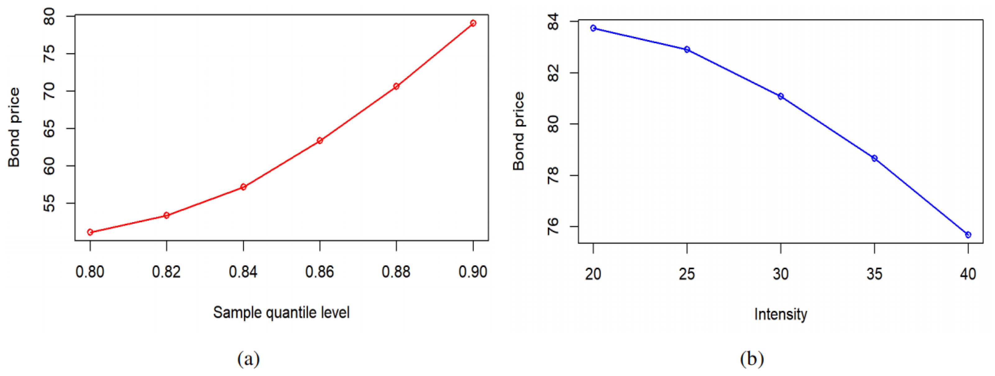
Finally, the price of the CAT bond, as the present value of all future cashflows, denoted by P t , is given by
P t = s = t + 1 T E C t , s p ( t , s ) + E F t , T · p ( t , T ) ,
where p ( t , s ) represents the discount factor at time t of the zero-coupon bond with a redemption value of 1 at time s , t < s T , given by
p ( t , s ) = E exp t s r ( u ) d u
with interest rate process { r ( t ) , t 0 } . In the following, we consider a CIR model for the interest rate risk, which will lead to an explicit expression of the discount factor.
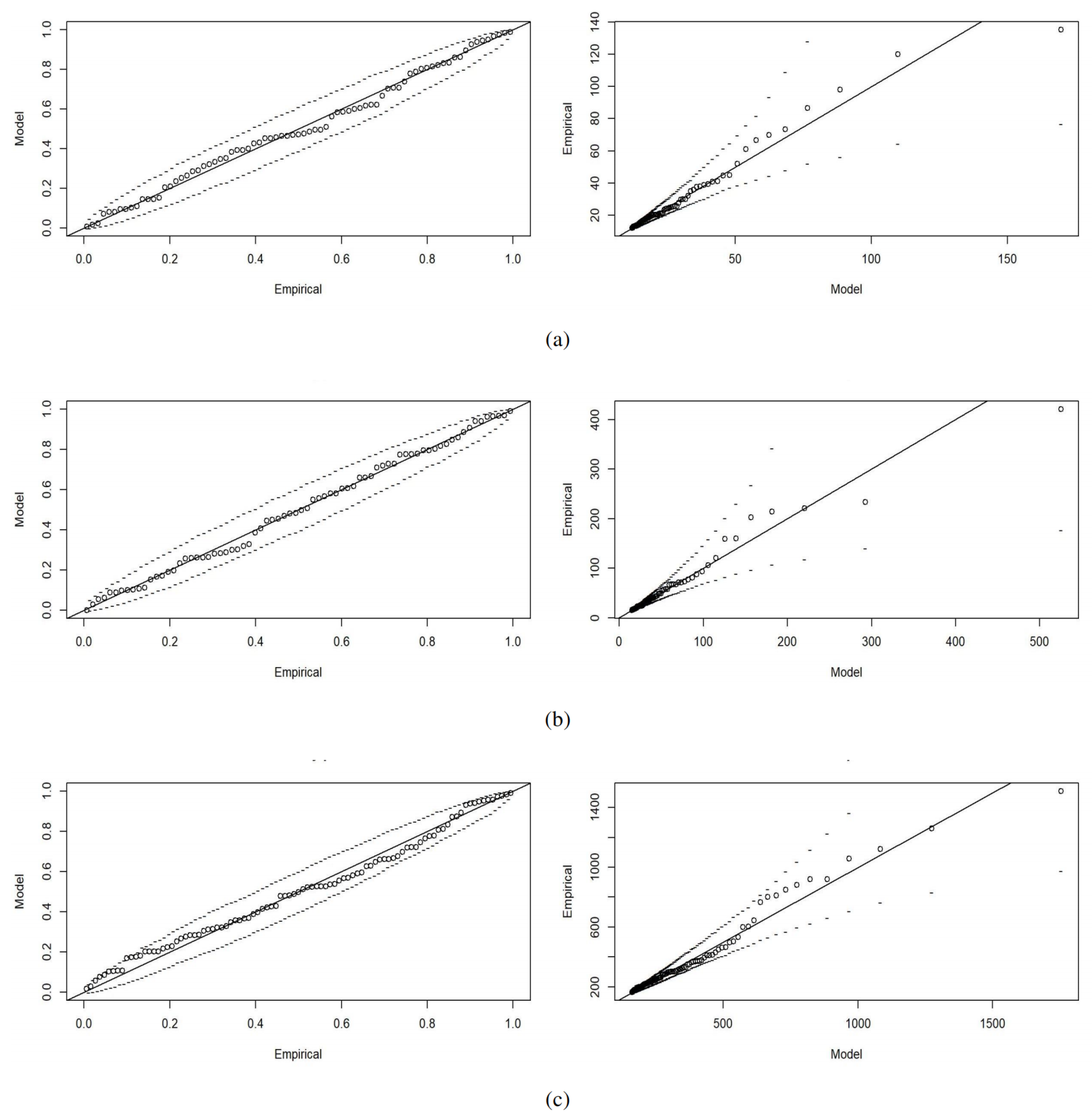
2.2. Interest Rate Model

In our study, we adopt the Cox–Ingersoll–Ross (CIR) model to describe the continuous-time interest rate process { r ( t ) , t 0 } (Cox et al. 1985). The CIR model offers specific advantages over the Vasicek interest rate model, such as its simplicity, ease of handling, mean-reverting behavior, and avoidance of negative interest rates (Mistry and Lombardi 2022; Vasicek 1977). It satisfies the following stochastic differential equation under the risk-neutral probability measure:
d r ( t ) = k θ r ( t ) d t + ε r ( t ) d W t ,
where k > 0 is the speed of mean reverting, ε > 0 is the volatility parameter, θ > 0 is the long-run mean of the interest rate, and { W t , t 0 } denotes the standard Wiener process. Consequently, the discount factor p ( t , T ) is given by
p ( t , T ) = A ( t , T ) e B ( t , T ) r ( t ) ,
where
A ( t , T ) = 2 η e ( κ + η ) ( T t ) / 2 ( κ + η ) e η ( T t ) 1 + 2 η 2 κ θ / ε 2 , B ( t , T ) = 2 e η ( T t ) 1 ( κ + η ) e η ( T t ) 1 + 2 η , η = κ 2 + 2 ε 2 .

2.3. POT Model

The extreme value theory plays an important role in analysing statistical patterns of extreme-value events. There are two typical approaches to extract the extreme samples: the block maximum (BM) method and the peaks-over-threshold (POT) model. As the POT model can make full use of the extreme-value data in comparison with the BM model, it is widely used in the fields of insurance, hydrology, and finance (Ma et al. 2021).
Suppose that X 1 , X 2 , , X n , is a random sample from parent X F ( x ) , i.e., the X i values are independent and identically distributed with a common distribution function (df) F ( x ) . Given a threshold u, the distribution F u ( y ) of the excess Y [ u ] = X u | X > u is thus given by
F u ( y ) = P X u y X > u = P u < X y + u P X > u = F ( y + u ) F ( u ) 1 F ( u ) , y > 0 .
For sufficiently high thresholds, Pickands (1975) pointed out that the distribution of the threshold-excess threshold Y [ u ] can be approximated by a generalized Pareto (GP) distribution G ξ , σ ( · ) , i.e., for the right endpoint x * = sup { x R : F ( x ) < 1 }
lim u x * sup 0 y x * u F u ( y ) G ξ , σ ( y ) = 0 .
Therefore, the tail distribution function F ¯ ( x ) = 1 F ( x ) of X can be approximated by
F ¯ ( x ) = F ¯ ( u ) F ¯ u ( x u ) F ¯ ( u ) G ¯ ξ , σ ( x u ) , x > u .
Here ξ R and σ > 0 are the shape and scale parameters of the GP distribution G ξ , σ ( y ) = 1 [ 1 + ξ y / σ ] 1 / ξ , y > 0 . In practice, the exceedance probability F ¯ ( x ) gives the insight into the potential risk. Its estimate can be obtained through the extrapolation approach via Equation (7): we obtain the approximate tail probability of the GP model using the maximum likelihood estimation of ξ , σ based on the excesses ( x ( i ) u ) with x ( 1 ) x ( n u ) exceeding the threshold u and the estimate of F ¯ ( u ) as n u / n . Theoretically, the threshold u can be determined by minimizing the mean square error of the Hill estimator of ξ 
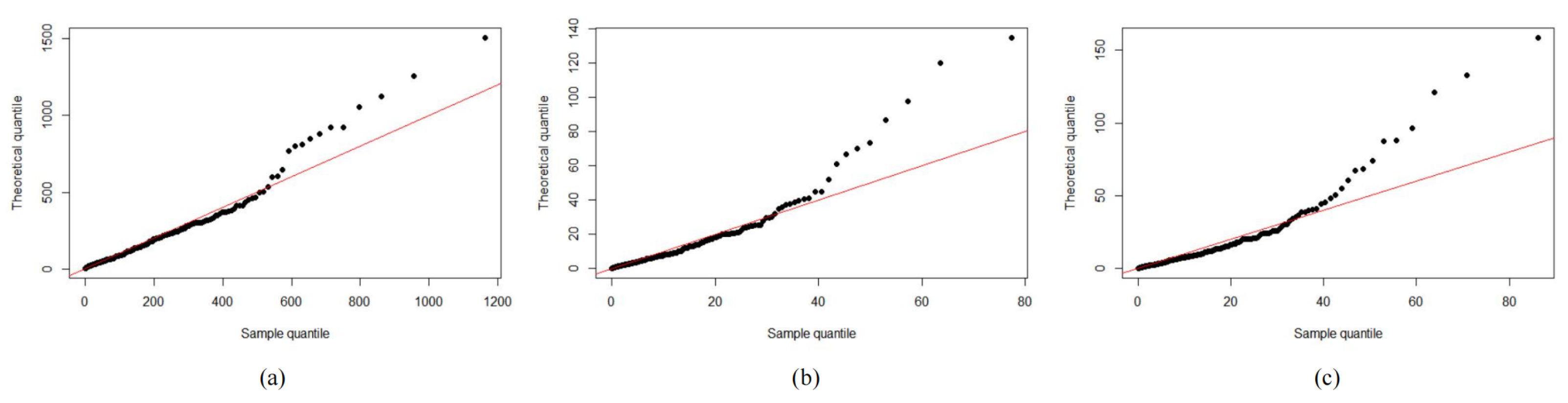
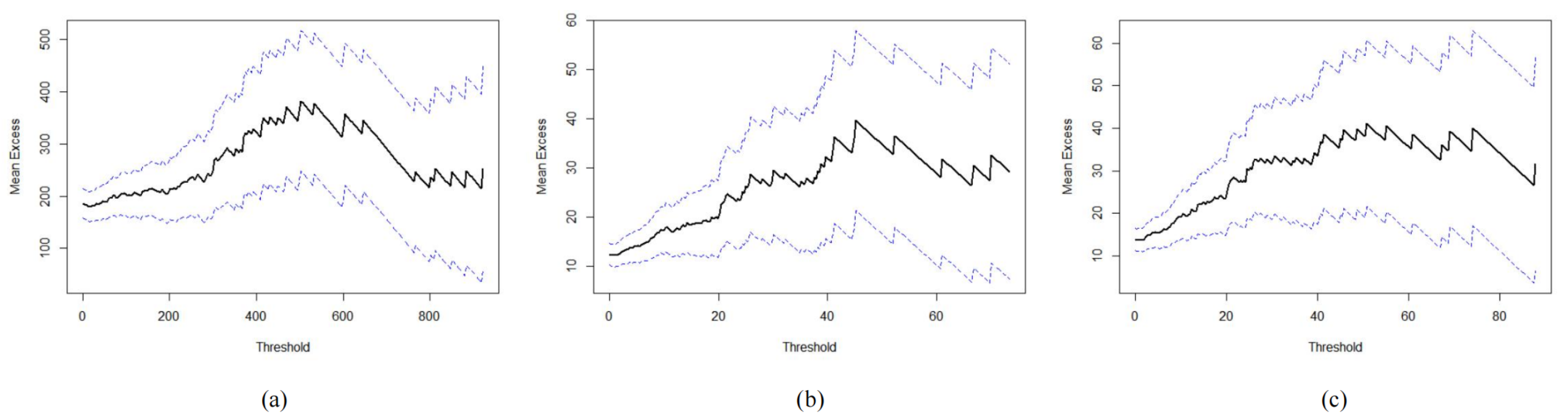
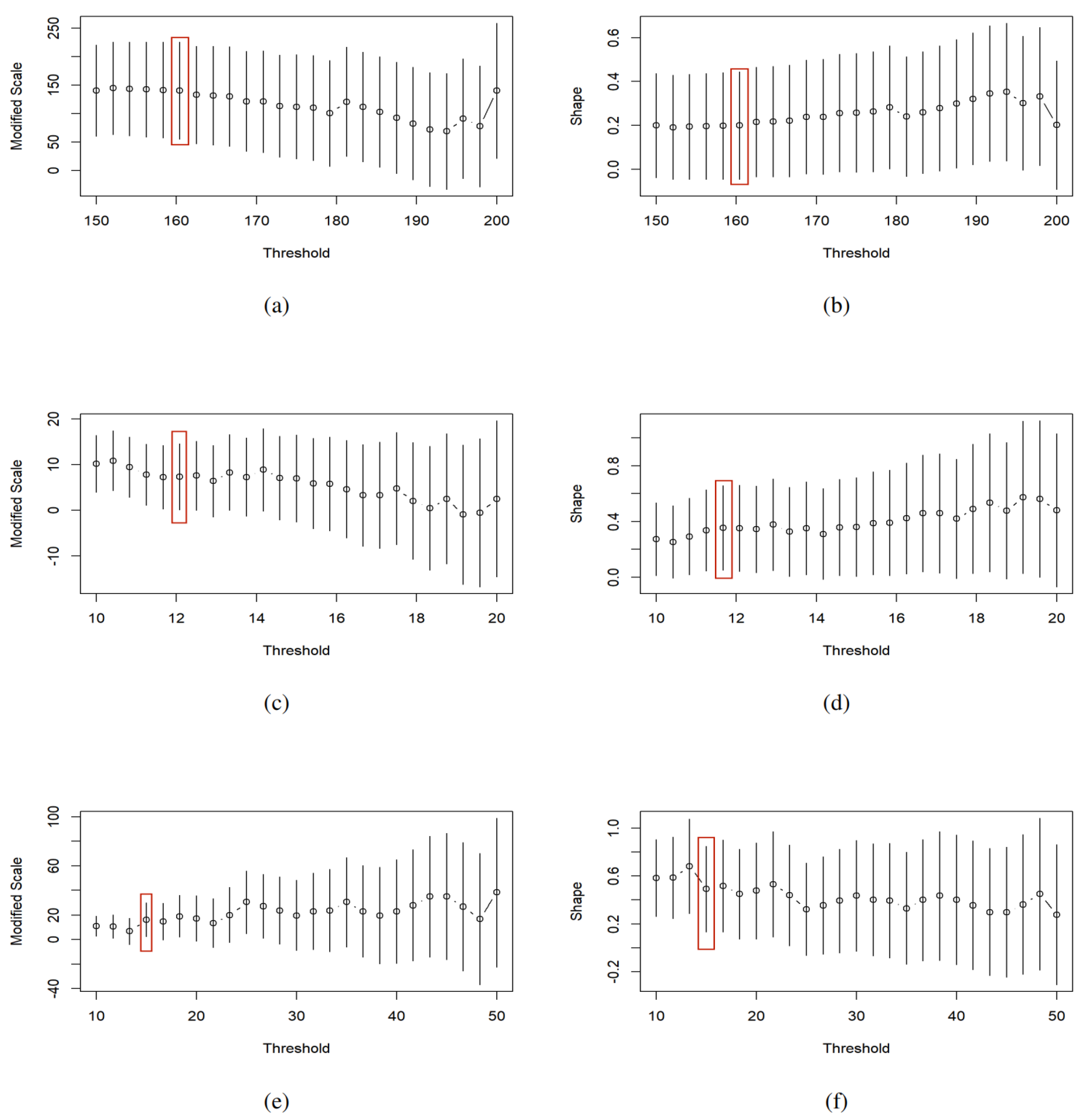
, balancing the model bias and variance. A common graphical approach to the determination of the threshold is to check both the linearity of the empirical mean excess function
e n ( u ) = 1 n u i = 1 n u x ( i ) u
and its derived stable estimates of both scale and shape parameters.

2.4. Copula

The concept of a copula, proposed by Abe (1973), serves as a tool for describing the dependence structure among the marginal variables. Namely, for a joint distribution G ( x 1 , , x m ) with marginal df G i for the ith component, the copula C is thus determined by
C ( u 1 , , u m ) = G ( G 1 1 ( u 1 ) , , G m 1 ( u m ) ) , ( u 1 , , u m ) [ 0 , 1 ] m .
Table 2 lists common Archimedean copulas, including the Clayton, Gumbel, and Frank copulas, with a convex and decreasing generator ϕ ( t ) : [ 0 , 1 ] ( 0 , ) satisfying ϕ ( 1 ) = 0 . Its tail dependence is controlled by the parameter θ and its copula is given by
C u 1 , , u m = ϕ 1 i = 1 m ϕ u i .
Given the analytic tractability of Archimedean copulas, they are widely applied in insurance, finance, hydrology, survival analysis, etc. In this paper, we consider hierarchical (or nested) Archimedean copulas representing the different dependence among the components (Hofert 2010). Namely, the nested Archimedean copula is of the form
C ( u 1 , , u m ) = C o u t e r C i n n e r u 1 , , u k ; θ 1 , u k + 1 , , u m ; θ 2 ,
where the inner and outer copulas could be one of the three Archimedean copulas in Table 2. The tail dependence could be measured by the parameters θ 1 and θ 2 . As shown in Charpentier and Segers (2009), the larger θ involved in the Gumbel, Clayton, or Frank copulas indicates a stronger dependence among these variables.
Combining the above pricing model and statistical model, this paper derives a rainstorm catastrophe bond. An empirical analysis together with a numerical analysis is given in Section 3.

3. Empirical Analysis and Numerical Analysis

To illustrate our pricing mechanism, this section develops the pricing of a severe rainstorm in China based on all recorded 245 major rainstorms in China during 2006–2020 and three main hazard indicators from the China Statistical Yearbook of Natural Disasters. These indicators cover all the disaster indicators, namely, the affected population (AP) accumulating the number of deaths, missing, emergency re-locations, and people with drinking water damaged; the crop affected area (CAA), reflecting both the cropland flooding area and its harvest-affected area; and the direct economic loss (DEL) adjusted with the Consumer Price Index (CPI) in 2020, summing the damaged losses of collapsed/damaged houses and other properties multiplied by its damaged ratio.
In what follows, we will first present the descriptive statistics of our triple of trigger indicators ( X 1 , X 2 , X 3 ) representing AP, CAA, and DEL in Section 3.1. The non-normality of these indicators motivates us to split the full range of the data into bulk and tail parts using classical parametric models and a peaks-over-threshold (POT) approach in Section 3.2, followed by the investigation of the joint distribution functions for disaster indicator data using a nested Archimedean copula in Section 3.3. The ARMA model is used to predict the disaster intensity over the next 3 years in Section 3.4. Monte Carlo simulation of the CAT bond price is carried out in Section 3.5. Here, we take the retention functions of f , h , and g in Equations (1)∼(3) as the same as the average or maximum function unless stated otherwise. That is,
α t = 1 N ( t ) N ( t 1 ) j = N ( t 1 ) + 1 N ( t ) i = 1 m 1 x i j u i + x i j . β t = 1 N ( t ) N ( t 1 ) j = N ( t 1 ) + 1 N ( t ) 1 i 1 < i 2 m 1 x i 1 j u i 1 + x i 1 j · x i 2 j u i 2 + x i 2 j , γ t = 1 N ( t ) N ( t 1 ) j = N ( t 1 ) + 1 N ( t ) 1 i 1 < i 2 < i 3 m 1 x i 1 j u i 1 + x i 1 j · x i 2 j u i 2 + x i 2 j · x i 3 j u i 3 + x i 3 j
and
α t = max j = N ( t 1 ) + 1 N ( t ) i = 1 m 1 x i j u i + x i j . β t = max j = N ( t 1 ) + 1 N ( t ) 1 i 1 < i 2 m 1 x i 1 j u i 1 + x i 1 j · x i 2 j u i 2 + x i 2 j , γ t = max j = N ( t 1 ) + 1 N ( t ) 1 i 1 < i 2 < i 3 m 1 x i 1 j u i 1 + x i 1 j · x i 2 j u i 2 + x i 2 j · x i 3 j u i 3 + x i 3 j .

3.1. Descriptive Analysis of Trigger Indicators

We can see from Table 3 that the averages of all three main indicators are far larger than their respective medians. Moreover, both the skewness and the kurtosis of these indicators, which are far larger than 0 and 3, respectively, indicate that the right-skewed pattern of these indicators have possible heavy tails. This is graphically consistent with the exponential QQ plots in Figure 2 with a downward convex deviation from the theoretical straight line.

3.2. POT-Based Tail Analysis of Trigger Indicators

In order to determine the threshold levels ( u 1 , u 2 , u 3 ) of the triple of indicators ( X 1 , X 2 , X 3 ) , we examine the mean residual life plots in Figure 3 (see Equation (8) for details). We determine first the threshold u 1 for the affected population X 1 . The possible range of the threshold is detected to be in the interval of ( 150 , 200 ) according to the sample mean residual plot with a linear trend (see Figure 3a), and then we investigate the stability of the estimations of the scale and shape parameters involved in the generalized Pareto model of the threshold excesses of AP in Figure 4a,b. Consequently, the attachment level u 1 = 160 is determined for the affected population (AP). Similar arguments are given to the attachment levels of u 2 = 12 for the crop affected area (CAA) and u 3 = 15 for the direct economic loss (DEL).
We model the probability distribution of our trigger indicators using the full range of the data, with sufficient flexibility for separate control over the bulk and tail features. Different from Chao and Zou (2018), we consider the Beta-GP models for the scaled non-exceedances and threshold excesses, namely,
X i u i | X i > u i G ( y ) = 1 1 + ξ y σ 1 / ξ , y > 0 , for   threshold   excesses , X i * = X i m i u i m i B e t a a , b ( y ) = 1 B ( a , b ) y a 1 ( 1 y ) b 1 , 0 < y < 1 , for   non-exceedances ,
where ( m 1 , m 2 , m 3 ) = ( 1.6 , 0.005 , 1.011 ) are the sample minima of the trigger indicators of AP, CAA, and DEL, respectively, given in Table 4, and ( u 1 , u 2 , u 3 ) = ( 160 , 12 , 15 ) are given by the mean residual plots and parameter stability plots. All maximum likelihood estimations of the parameters involved in the Beta-GP models are shown in Table 4. We see that both CAA and DEL possess heavy tails with 95% confidence intervals of the shape parameters of ( 0.03 , 0.64 ) and ( 0.13 , 0.84 ) , respectively, while the estimated shape parameter for AP excesses is 0.197, showing a certain power-decaying tail. Moreover, we examine the model goodness-of-fit using a Chi-square test and obtain that all the p-values are larger than 0.246, confirming that the Beta-GP model agrees with the observed trigger indicators. Intuitively, Figure 5 illustrates the appropriateness of the GP model of the threshold exceedances for each trigger indicator, since both the PP plots and QQ plots show that almost all points are around the straight line.
To conclude, the fitted distributions F i , i = 1 , 2 , 3 corresponding to the trigger indicators of the affected population (AP), the crop affected area (CAA), and the direct economic loss (DEL) are given below
F i ( x ) = 1 n u i n G ¯ ξ i , σ i ( x u i ) , x > u i , 1 B ( a i , b i ) 0 ( x m i ) / ( u i m i ) t a i 1 ( 1 t ) b i 1 d t , x u i ,
where n = 245 and the threshold ( u 1 , u 2 , u 3 ) , the excess numbers ( n u 1 , n u 2 , n u 3 ) , the sample minina ( m 1 , m 2 , m 3 ) , and other parameters for the Beta-GP model are given by Equation (12) and Table 4.
Given the distributions of each trigger indicator in Equation (13), it remains to discuss the dependence via nested Archimedean copula in the following section in order to illustrate our multiple-event-triggered pricing mechanism in Section 3.5.

3.3. Dependence Anaylsis of Trigger Indicators Based on Nested Archimedean Copula

We shall investigate first the non-exchangeable dependence among the trigger indicators through the Spearman rank correlation ρ . The Spearman ρ for (AP, CAA), (AP, DEL), and (CAA, DEL) are 0.771, 0.554, and 0.515, respectively. We see that all three pairs demonstrate a certain degree of dependence, with a stronger dependence within (AP, CAA) than between them. This motivates us to describe the dependence using a nested Archimedean copula, with an inner copula for (AP, CAA) with Archimedean parameter θ 1 and DEL placed into the outer Archimedean copula with parameter θ 2 (see Equation (9)).
Next, to model the dependence structure using a nested Archimedean copula, we construct a uniformly distributed transformation of the raw data according to the marginal analysis in Section 3.2, i.e., a straightforward application of Equation (13) given by
u ˜ i j = F i ( x i j ) , i = 1 , 2 , 3 , j = 1 , 2 , , 245 .
Finally, we examine the dependence structure using a nested Archimedean copula with both the inner and outer copula being one of the Gumbel, Clayton, and Frank copulas listed in Table 2. We suppose that
( u ˜ 1 j , u ˜ 2 j , u ˜ 3 j ) i . i . d . C o u t e r ( C i n n e r ( u ˜ 1 j , u ˜ 2 j ; θ 1 ) , u ˜ 3 j ; θ 2 ) , j = 1 , 2 , , 245 .
We see from Table 5 that the maximum likelihood estimates of the inner parameter θ 1 are all larger than that of the outer parameter θ 2 , agreeing with the stronger dependence within the inner variables than between them. Moreover, we will select the most suitable copula based on the Kolmogorov–Smirnov (KS) test. We see that all nested Archimedean copulas fit the data well and the best nested Gumbel copula is determined with the minimal KS test value of 0.04 and the maximum p-value of 0.61.

3.4. Modelling of Annual Frequency of Rainstorms in China

Note that our pricing mechanism is of discrete form. It follows from Equation (4) that the proportion of the coupon and principal paid out depends not only on the severity of the disasters (thus, the trigger indicators) but also on the independent annual frequency of disasters. This was confirmed by our Pearson correlation analysis between the annual number of rainstorms and its resulting annual average of losses in terms of AP, CAA, and DEL, with values equal to 0.08 , 0.09 , and 0.1 , respectively. Due to the changing climate, the occurrence of major rainstorms becomes more and more frequent.The purpose of this section is to model the intensity of annual major rainstorms during 1986–2020 in China using an auto-regressive moving average (ARMA) model so as to forecast the frequency in the next three years, i.e., 2021–2023. The relevant data are from the China Statistical Yearbook of Natural Disasters.
The stationarity of the time series Λ t is validated by the augmented Dickey–Fuller (ADF) test at a significance level of 0.05. Next, we determine the autoregressive order and moving-average order as p = 1 , q = 3 , respectively, by the position of the lag cutoff in the partial autocorrelation function (PACF) and ACF plots in Figure 6. Thus, the ARMA(1, 3) model is selected for modelling the annual intensity of major rainstorms in China and the maximum likelihood estimates of the parameters involved are obtained as ( ϕ 1 , θ 1 , θ 2 , θ 3 ) = ( 0.816 , 0.268 , 0.240 , 0.748 ) .
The Jarque–Bera (JB) test with a p-value of 0.08 confirms the normality assumption of the residuals e k , given in Equation (A1) in the ARMA model, and its i.i.d. assumption is verified by the Ljung–Box (LB) test with p = 0.502 . Before we apply this model for prediction, we carried out an F-test, which confirmed the goodness of fit with p = 0.003 . Consequently, the straightforward application of ARMA(1,3) to the intensity measures for 2021, 2022, and 2023 predicts ( 41.86 , 41.56 , 39.39 ) a general upward trend in intensity for the next three years, as shown in Figure 7, which will be used in Section 3.5 below for the numerical analysis of pricing sensitivity.

3.5. Pricing of CAT Bond and Numerical Analysis

This section will focus on the CAT bond pricing based on our pricing mechanism in Equation (5) and the basic analyses of major rainstorms we conducted in Section 3.1, Section 3.2, Section 3.3 and Section 3.4. In the current pricing mechanism, we suppose mutual independence among interest rate, disaster indicators, and counting process (Chao and Zou 2018; Goda 2021; Ibrahim et al. 2022; Reshetar 2008). This facilitates Monte Carlo simulations in both the numerical analysis and the empirical analysis. In practice, there might be weak and ignorable dependence between the financial market and natural disaster risks, which attracts investors for the benefit of diversification of their investments. On the other hand, the dependence assumption between the frequency and severity of disasters is more likely to bring about model mis-specification. In what follows, we consider a T-year period CAT bond with a principal of F = C N Y 100 and a fixed coupon rate R = 3.5 % . Note that the explicit expectation in Equation (5) is not available. We thus simulate the price of the CAT bond and estimate it as the average of the simulated price. The steps of the simulation are outlined as follows.
(1)
Generate T random numbers N 1 , N 2 , , N T independently from a Poisson distribution with intensity measure Λ 1 , Λ 2 , , Λ T , standing for the number of major rainstorms in year 1 , 2 , , T . Here, ( Λ 1 , Λ 2 , , Λ T ) can be provided by the ARMA(1, 3) model in Section 3.4.
(2)
Based on the marginal distribution in Equation (13) and the nested Frank copula in Equation (14) with parameters given in Table 4 and Table 5, we generate a sample of ( x 1 k , x 2 k , x 3 k ) of size N j for year j , 1 j T as
x i k = F i 1 ( u ˜ i k ) , i = 1 , 2 , 3 , k = l = 1 j 1 N l + 1 , , l = 1 j N l .
(3)
We suppose that the stochastic interest rate process { r ( t ) , t 0 } follows the CIR model stated in Equation (6), and the parameter estimates involved are obtained through maximum likelihood estimation based on one-year seven-day interest rate data for 2021, available at the Shanghai Interbank Offered Rate. We select the interest rate on 6 January 2021 as the initial interest rate, i.e.,
d r ( t ) = 0.2 0.05 r ( t ) d t + 0.05 r ( t ) d W t , r ( 0 ) = 2.962 % .
We simulate the interest risk to give the discount factor p ( t , T ) .
(4)
Given a trigger level ( u 1 , u 2 , u 3 ) , we calculate the price of the CAT bond based on the cashflows in Equation (4) and the interest risk model in Equation (15).
We repeat m = 10 4 all the simulation steps above and obtain the sample mean of the price P t of a T-year CAT bond bought in year t = 0 , 1 , , T 1 . In the following, we will discuss the pricing sensitivity in the maturity period, the trigger level, and the trigger indicators.
Price sensitivity in maturity period. Table 6 shows a T-year CAT bond triggered by the triple of trigger indicators (AP, CAA, DEL) with trigger level ( u 1 , u 2 , u 3 ) being the sample 90% quantile. The bond price decreases at the maturity period T and further, the downward trend in the bond price gradually increases. As the bond is issued for a long maturity period, future disasters might be more severe and frequent, causing a larger magnitude of triggered events and thus a smaller proportion of the coupon and principal retained. Consequently, a lower price is obtained for a medium-term CAT bond. Meanwhile, for a given maturity period T = 2 or 3, the CAT bond might be sold in different years during the bond issue period. We see that the price of a bond purchased in an earlier year is higher, as the potential risk of major rainstorms might be lower in the previous few years and the coupon and principal are more likely to remain. Therefore, the pricing mechanism is fairly attractive in terms of raising capital for the purpose of reinsurance. We see further that the CAT bond prices vary in coupon–principal retention functions. Clearly, the coupon and principal remaining based on the annual average retention level in Equation (10) are not larger than that based on the annual maximum retention level in Equation (11), which results in the lower price of the former. Hence, our functional mechanism of the retention levels provides sufficient flexibility to the CAT bond issuers.
Price sensitivity to trigger level and intensity measure of major rainstorms. An appropriate trigger level is important for balancing the benefits between the investors and the bond issuers by means of the CAT bond price. In general, both the trigger levels and the intensity measures are determined by the severity and frequency of the potential disasters (here rainstorms), which can cause a change in the CAT bond price via the wiped-off coupon and principal in Equation (4). Clearly, we see from Figure 8 that the bond prices are positively correlated with the trigger levels but negatively associated with the intensity measures. Indeed, as the trigger level increases, a bond is less likely to be triggered and thus the coupon and principal retention level will increase, leading to an increase in the CAT bond price. In contrast, if major rainstorms occur more frequently with a larger intensity measure, the triggered indicators may accumulate a small amount of coupon and principal retained, thus causing a decrease in bond prices.
Price sensitivity in the selection of trigger indicators. As mentioned before, the multiple-event-triggered CAT bond receives increasing attraction from both investors and CAT issuers. In Table 7, we compare the one-year bond prices with different pairs of trigger indicators under our pricing mechanism in Equation (5). Apparently, the three-event-triggered CAT bond is issued with a lower price than that of two-event-triggered ones. This is because the smaller trigger probability of concurrent trigger events leads to a lower expectation of discounted cashflows. Additionally, the principal might be half-returned in case all three indicators are triggered (recalling the utilization of γ t ).

4. Conclusions and Extensional Discussions

In this paper, a multiple-event-triggered CAT bond pricing model is designed and a pricing formula is derived based on the copula–POT model. Our pricing model is more flexible and of more practical significance in terms of possessing a dynamic association between the coupon and principal paid off, whose magnitude varies in both the severity and frequency of the potential disasters. This model may provide a certain reference for the pricing research and subsequent practical application of catastrophe bonds. Although the multi-event trigger mechanism involves more elements and more complex processes and requires higher technical capabilities, the multiple-event-triggered bonds receive increasing attraction due to their low moral hazard and trigger risk (Chao and Zou 2018; Ibrahim et al. 2022; Wei et al. 2022). Meanwhile, it turns out that the CAT bond price decreases in the bond maturity period in the simulation, and it is negatively correlated with the trigger level and positively correlated with the catastrophe intensity.
The pricing mechanism depends on the joint distribution of the target indicators caused by the disaster (Goda 2021). In real life, catastrophic risks involve multiple disasters over many regions. Thus, a forthcoming research direction is to design a regional CAT bond pricing model that incorporates spatio-temporal extremes and the interaction of simultaneous disasters. Furthermore, we may bring the insights from Eling and Wirfs (2019) and incorporate relevant covariates such as the economic development level and the vulnerability to real rainstorms for estimating the local parameter of the POT model, which thus enables a region-specific pricing mechanism in practice. In addition, to relax the independence assumption among the interest rate risk, disaster indicators, and counting process might be more realistic in the CAT bond pricing models, with potential complexity regarding the pricing simulations and statistical tests of the possible dependence structure. Furthermore, the specific assumptions should be carefully verified since otherwise it is more likely to result in a model mis-specification issue. In practice, there might be weak dependence between the financial market risk and disaster risk, which hopefully enables the investors to be protected from the diversification investment.

Author Contributions

Y.T. and C.L. proposed the research objectives and constructed the pricing model; Y.T. collected the data and conducted the model simulations; C.L., C.W. and Y.Z. contributed to the writing/revisions of the manuscript. All authors have read and agreed to the published version of the manuscript.

Funding

This project was funded by the Research Development Fund at XJTLU (RDF1912017) and the Post-graduate Research Scholarship (PGRS2112022) and Jiangsu Qinglan Talent in 2022.

Data Availability Statement

The data that support the findings of this study are available from the China Statistical Yearbook of Natural Disasters, but restrictions apply to the availability of these data, which were used under license for the current study and so are not publicly available. The data are, however, available from the authors upon reasonable request and with permission of the China Statistical Yearbook of Natural Disasters.

Acknowledgments

The authors would like to thank the referees and associate editor for their constructive suggestions, which significantly improved this contribution.

Conflicts of Interest

The authors declare no conflict of interest.

Appendix A

Appendix A.1. Counting Process

The homogeneous Poisson process has smooth independent increments. When 0 t 1 < t 2 < < t k , the distribution of the increment N ( t j ) N ( t j 1 ) depends only on the length of the time interval Δ t j = t j t j 1 , not on the specific starting time point of t j , and the increments over non-overlapped intervals are independent of each other. In this case, if we denote by λ the average number of disasters per time unit interval, then
P N ( t ) = k = ( λ t ) k exp ( λ t ) k ! , k = 0 , 1 , 2 , .
The non-homogeneous Poisson process (NHPP) allows the instantaneous intensity density λ ( t ) to be a function of t. Namely, the number of disasters up to time t follows a Poisson distribution with mean Λ ( t ) satisfying
Λ ( t ) = 0 t λ ( x ) d x .
In general, the number of disasters in the time interval ( s , s + Δ t ] follows a Poisson distribution with mean
Λ ( s + Δ t ) Λ ( s ) = s s + Δ t λ ( x ) d x .

Appendix A.2. ARMA Model

ARMA models are used for time-series analysis and forecasting by modeling the autocorrelation and moving average of the series. ARIMA models can be reduced to an ARMA process through differencing. This transforms the non-stationary series into a stationary one, which can be modeled using an ARMA process. The ARMA model for the intensity of annual rainstorms can be stated as follows (Ibrahim et al. 2022):
Λ k = μ + ϕ 1 Λ k 1 + + ϕ p Λ k p + θ 1 e k 1 + + θ q e k q + e k ,
where Λ t = Λ ( t + 1 ) Λ ( t ) represents the intensity measure of annual rainstorms in year j , j = 1 , 2 , , k ; p and q represent autoregressive and moving-average order, respectively; and e k represents the random error. The assumptions in the ARMA ( p , q ) are as follows:
  • The random errors e k are independent and normally distributed with zero mean and constant variance, denoted by e k i . i . d . N ( 0 , σ 2 ) ,
  • The sequence Λ k are weakly stationary, that is, k , E Λ k = μ Λ and Var Λ k = σ Λ 2 .

Appendix A.3. Proof of Proposition 1

Proof. 
Without loss of generality, we will show the proposition for t = 1 , N ( 1 ) = n , and all the observed indicator samples ( x 1 j , x 2 j , , x m j ) , j = 1 , n are given. Recall that the threshold ( u 1 , , u m ) is given to be positive.
(i).
It follows by the fact that 0 ( x u ) + < x for x , u > 0 that
a i j : = x i j u i + x i j [ 0 , 1 )
and 1 a i j ( 0 , 1 ] . Hence,
s j = i = 1 m ( 1 a i j ) ( 0 , 1 ] .
And s j = 1 if and only if a 1 j = a 2 j = = a m j = 0 , that is, x i j < u i for all 1 i m . Denote further
a i 1 j = x i 1 j u i 1 + x i 1 j , a i 2 j = x i 2 j u i 2 + x i 2 j , a i 3 j = x i 3 j u i 3 + x i 3 j .
We have
s j * = 1 i 1 < i 2 m ( 1 a i 1 j a i 2 j ) , s j * * = 1 i 1 < i 2 < i 3 m ( 1 a i 1 j a i 2 j a i 3 j ) ,
yielding that s j * < 1 is equivalent to there being a pair ( a i 1 j , a i 2 j ) such that a i 1 j , a i 2 j > 0 . Hence, both indicators x i 1 j and x i 2 j are exceeding the threshold u i 1 and u i 2 in the j-th disaster. Similarly, s j * * < 1 if and only if there are at least three indicators over its threshold concurrently.
(ii).
It follows from the fact that a i j [ 0 , 1 ) that
a i 1 j a i 1 j a i 2 j a i 1 j a i 2 j a i 3 j and 0 < 1 a i 1 j 1 a i 1 j a i 2 j 1 a i 1 j a i 2 j a i 3 j 1 .
In addition, we have
i : a i j > 0 1 a i j ( i 1 , i 2 ) : a i 1 j a i 2 j > 0 1 a i 1 j a i 2 j ( i 1 , i 2 , i 3 ) : a i 1 j a i 2 j a i 3 j > 0 1 a i 1 j a i 2 j a i 3 j ,
i.e., 0 < s j s j * s j * * 1 . Moreover, since f is a component-wise, non-decreasing, non-negative, and right-continuous function from [ 0 , 1 ] N to ( 0 , 1 ] , we have
0 < f ( s 1 , s 2 , , s n ) f ( s 1 * , s 2 * , , s n * ) f ( s 1 * * , s 2 * * , , s n * * ) 1 , n 1 .
Consequently, 0 < α t β t γ t 1 holds when f = g = h .
(iii).
For a disaster year with more severe and frequent catastrophic events, the excess proportion of a i j increases with more terms of a i j positive, leading to a smaller value of s j . Finally, the component-wise non-decreasing monotonicity of f indicates a small value of α t . Similar arguments apply for β t and γ t .

References

  1. Aase, Knut. 1999. An equilibrium model of catastrophe insurance futures and spreads. The Geneva Papers on Risk and Insurance Theory 24: 69–96. [Google Scholar] [CrossRef]
  2. Abe, Sklar. 1973. Random variables, joint distribution functions, and copulas. Earthquake Spectra 9: 449–60. [Google Scholar]
  3. Anantapadmanabhan, C. S. 1971. Some statistical aspects of catastrophic risks. ASTIN Bulletin: The Journal of the IAA 5: 307–13. [Google Scholar] [CrossRef]
  4. Braun, Alexander. 2016. Pricing in the primary market for CAT bonds: New empirical evidence. Journal of Risk and Insurance 83: 811–47. [Google Scholar] [CrossRef]
  5. Chao, Wen, and Huiwen Zou. 2018. Multiple-event catastrophe bond pricing based on CIR-Copula-POT model. Discrete Dynamics in Nature and Society 2018: 5068480. [Google Scholar] [CrossRef]
  6. Charpentier, Arthur, and Johan Segers. 2009. Tails of multivariate Archimedean copulas. Journal of Multivariate Analysis 100: 1521–37. [Google Scholar] [CrossRef]
  7. Chen, Junfei, Guiyun Liu, Liu Yang, Quanxi Shao, and Huimin Wang. 2013. Pricing and simulation for extreme flood catastrophe bonds. Water Resources Management 27: 3713–25. [Google Scholar] [CrossRef]
  8. Cox, John C., Jonathan E. Ingersoll, and Stephen A. Ross. 1985. An intertemporal general equilibrium model of asset prices. Econometrica 53: 363–84. [Google Scholar] [CrossRef]
  9. Cox, Samuel H., and Hal W. Pedersen. 2000. Catastrophe risk bonds. North American Actuarial Journal 4: 56–82. [Google Scholar] [CrossRef]
  10. Cummins, David J. 2008. CAT bonds and other risk-linked securities: State of the market and recent developments. Risk Management and Insurance Review 11: 23–47. [Google Scholar]
  11. Deng, Guoqu, Shiqiang Liu, Li Li, and Chushi Deng. 2020. Research on the pricing of global drought catastrophe bonds. Mathematical Problems in Engineering 2020: 3898191. [Google Scholar] [CrossRef]
  12. Eling, Martin, and Jan Wirfs. 2019. What are the actual costs of cyber risk events? European Journal of Operational Research 272: 1109–19. [Google Scholar] [CrossRef]
  13. Goda, Katsuichiro. 2021. Multi-hazard parametric catastrophe bond trigger design for subduction earthquakes and tsunamis. Earthquake Spectra 37: 1827–48. [Google Scholar] [CrossRef]
  14. Hofert, Marius. 2010. Sampling Nested Archimedean Copulas with Applications to CDO Pricing. Ph.D. thesis, Universität Ulm, Ulm, Germany. [Google Scholar]
  15. Ibrahim, Riza Andrian, Sukono, and Herlina Napitupulu. 2022. Multiple-trigger catastrophe bond pricing model and its simulation using numerical methods. Mathematics 10: 1363. [Google Scholar] [CrossRef]
  16. Karagiannis, Nikolaos, Hirbod Assa, Athanasios A. Pantelous, and Calum G. Turvey. 2016. Modelling and pricing of catastrophe risk bonds with a temperature-based agricultural application. Quantitative Finance 16: 1949–59. [Google Scholar] [CrossRef]
  17. Leppisaari, Matias. 2016. Modeling catastrophic deaths using EVT with a microsimulation approach to reinsurance pricing. Scandinavian Actuarial Journal 2016: 113–45. [Google Scholar] [CrossRef]
  18. Litzenberger, Robert H., David R. Beaglehole, and Craig E. Reynolds. 1996. Assessing catastrophe reinsurance-linked securities as a new asset class. Journal of Portfolio Management 23: 76–86. [Google Scholar] [CrossRef]
  19. Ma, Ning, Yanbing Bai, and Shengwang Meng. 2021. Return period evaluation of the largest possible earthquake magnitudes in mainland China based on extreme value theory. Sensors 21: 1424–8220. [Google Scholar] [CrossRef]
  20. McNeil, Alexander J. 1997. Estimating the tails of loss severity distributions using extreme value theory. ASTIN Bulletin: The Journal of the IAA 27: 117–37. [Google Scholar] [CrossRef]
  21. Mistry, Harsh K., and Domenico Lombardi. 2022. Pricing risk-based catastrophe bonds for earthquakes at an urban scale. Scientific Reports 12: 9729. [Google Scholar] [CrossRef] [PubMed]
  22. Nowak, Piotr, and Maciej Romaniuk. 2013. Pricing and simulations of catastrophe bonds. Insurance: Mathematics and Economics 52: 18–28. [Google Scholar] [CrossRef]
  23. Pauly, Mark V. 1968. The economics of moral hazard: Comment. The American Economic Review 58: 531–37. [Google Scholar]
  24. Pickands, James. 1975. Statistical inference using extreme order statistics. Annals of Statistics 3: 119–31. [Google Scholar]
  25. Reshetar, Ganna. 2008. Pricing of Multiple-Event Coupon Paying CAT Bond. Working Paper. Zürich: Swiss Banking Institute. [Google Scholar]
  26. Richter, Andreas, and Thomas C. Wilson. 2020. COVID-19: Implications for insurer risk management and the insurability of pandemic risk. The Geneva Risk and Insurance Review 45: 171–99. [Google Scholar] [CrossRef]
  27. Tang, Qihe, and Zhongyi Yuan. 2019. CAT bond pricing under a product probability measure with POT risk characterization. ASTIN Bulletin: The Journal of the IAA 49: 457–90. [Google Scholar] [CrossRef]
  28. Vasicek, Oldrich. 1977. An equilibrium characterization of the term structure. Journal of Financial Economics 5: 177–88. [Google Scholar] [CrossRef]
  29. Wei, Longfei, Lu Liu, and Jialong Hou. 2022. Pricing hybrid-triggered catastrophe bonds based on Copula-EVT model. Quantitative Finance and Economics 6: 223–43. [Google Scholar] [CrossRef]
  30. Woo, Gordon. 2004. A catastrophe bond niche: Multiple event risk. Paper presented at the NBER Insurance Workshop, Cambridge, UK, February 6–7. [Google Scholar]
  31. Zimbidis, Alexandros A., Nickolaos E. Frangos, and Athanasios A. Pantelous. 2007. Modeling earthquake risk via extreme value theory and pricing the respective catastrophe bonds. ASTIN Bulletin: The Journal of the IAA 37: 163–83. [Google Scholar] [CrossRef]
Figure 1. Flowchat of catastrophe bond.
Risks 11 00151 g001
Figure 2. Exponential QQ plots of (a) affected population (AP), (b) crop affected area (CAA), and (c) direct economic loss (DEL). The black dotted lines present concave features in the right tail, indicating a heavier tail than exponential distribution. Here the solid red line represents the exponential reference line.
Risks 11 00151 g002
Figure 3. The mean residual life plots for (a) affected population (AP), (b) crop affected area (CAA), and (c) direct economic loss (DEL). The solid black lines represent the mean residual life plot, and the blue dotted lines correspond to the 95% confidence intervals.
Risks 11 00151 g003
Figure 4. Parameter stability plots on the top for affected population (AP), in the middle for crop affected area (CAA), and on the bottom for direct economic loss (DEL). The shorter the bars are, the more stable the estimations of the parameters are. Here, (a,c,e) are for scale parameter σ and (b,d,f) for the shape parameter ξ . The red box indicates the selected threshold.
Risks 11 00151 g004
Figure 5. The PP plots (left) and QQ plots (right) for (a) affected population (AP), (b) crop affected area (CAA), and (c) direct economic loss (DEL). The solid lines represent the expected distribution, the dotted lines represent a 95% confidence interval, and the hollow circles represent the distribution of the observed data.
Risks 11 00151 g005
Figure 6. (a) Partial autocorrelation function (PACF) and (b) autocorrelation function (ACF) diagram for annual intensity of rainstorms in China during 1985−2020. The blue dashed lines represent the significance boundary at the 95% confidence interval.
Risks 11 00151 g006
Figure 7. Annual number of major rainstorms in China during 1985–2020; data are from the China Statistical Yearbook of Natural Disasters.
Risks 11 00151 g007
Figure 8. Price sensitivity of one-year CAT bond to (a) trigger levels and (b) disaster intensity measure Λ 1 = 20 , 25 , , 40 . Here the trigger level in (a) is the sample quantile at level q = 0.80 , 0.82 , , 0.90 for a given intensity measure in Step 1, while in (b) we fix the trigger level as its sample 90% quantile.
Risks 11 00151 g008
Table 1. Notation and its description involved in the pricing formula.
NotationDescription
FPrincipal
C t Coupon paid in year t , t = 1 , , T
RCoupon rate
N ( t ) Number of disasters up to year t
N t = N ( t ) N ( t 1 ) Number of disasters in year t
x i j The jth observation of the ith trigger indicator up to year t, j = 1 , , N ( t )
u i Attachment level of the ith trigger indicator, i = 1 , , m
Table 2. Common Archimedean copulas.
CopulaGenerator C ( u 1 , , u m ; θ ) Parameters
Gumbel ( ln t ) θ exp i = 1 m ln u i θ 1 / θ θ 1
Clayton t θ 1 θ i = 1 m u i θ m + 1 1 / θ θ 0
Frank ln e θ t 1 e θ 1 1 θ ln 1 + i = 1 m e θ u i 1 e θ 1 m 1 θ 0
Table 3. Descriptive statistics of affected population (AP) in millions, crop affected area (CAA) in million hectares, and direct economic loss (DEL) in billion yuan.
Trigger IndicatorsMaximumMinimumMeanMedianSkewnessKurtosis
AP1510.0001.600187.880116.7502.77112.678
CAA135.2000.00512.4927.0003.68920.458
DEL420.8161.01121.4118.0835.15437.823
Table 4. Estimates of the scale ( σ ) and shape ( ξ ) parameters in the GP models of the threshold excesses and the two parameters α and β in the Beta model B e t a α , β for the scaled bulk data below the threshold. The p-value based on a Chi-square test confirms that the Beta-GP model fits the data well.
GPBeta
Scale ( σ )95% CIShape ( ξ )95% CIp-Valueabp-Value
AP173.369(118.21, 226.38)0.197(−0.04, 0.44)0.2471.0161.3450.246
CAA11.771(7.41, 16.13)0.341(0.03, 0.64)0.2831.0761.6870.299
DEL23.538(13.96, 33.19)0.492(0.13, 0.84)0.2500.5821.1370.253
Table 5. Maximum likelihood estimates of the parameters involved in the inner and outer copulas in Equation (9). The Kolmogorov–Smirnov (KS) test and its p-value indicates that the best model is the nested Gumbel copula.
Inner and Outer Copula θ 1 (Inner) θ 2 (Outer)KS Testp-Value
Gumbel44.6822.800.060.12
Clayton9.584.350.120.35
Frank176.3487.600.040.61
Table 6. CAT bond pricing of major rainstorms in China purchased in year t and maturating in year T = 1 , 2 , 3 based on Equation (5). Here the trigger level ( u 1 , u 2 , u 3 ) is taken as the sample 90% quantile of (AP, CAA, DEL). The bond prices P t 1 and P t 2 are given based on the cashflows with an average retention level in Equation (10) and max retention level in Equation (11).
T = 1 T = 2 T = 3
t = 0 t = 0 t = 1 t = 0 t = 1 t = 2
Bond price P t 1 80.39270.88166.25556.00654.86552.321
Bond price P t 2 83.25973.21168.45058.81257.64953.984
Table 7. Comparison of one-year CAT bond price with different selections of multiple-event triggers under our pricing mechanism in Equation (5). The bond prices P t 1 and P t 2 are given according to the annual average and annual maximum retention functions in Equation (10) and Equation (11), respectively.
Trigger IndicatorAP-CAA-DELAP-CAAAP-DELCAA-DEL
Bond price P t 1 80.392248.755848.756148.7564
Bond price P t 2 83.259248.786948.787148.7873
Disclaimer/Publisher’s Note: The statements, opinions and data contained in all publications are solely those of the individual author(s) and contributor(s) and not of MDPI and/or the editor(s). MDPI and/or the editor(s) disclaim responsibility for any injury to people or property resulting from any ideas, methods, instructions or products referred to in the content.

