Pricing Pandemic Bonds under Hull–White & Stochastic Logistic Growth Model

Abstract

Pandemic bonds can be used as an effective tool to mitigate the economic losses that governments face during pandemics and transfer them to the global capital market. Once considered as an “uninsurable” event, pandemic bonds caught the attention of the world with the issuance of pandemic bonds by the World Bank in 2017. Compared to other CAT bonds, pandemic bonds received less attention from actuaries, industry professionals, and academic researchers. Existing research focused mainly on how to bring epidemiological parameters to the pricing mechanism through compartmental models. In this study, we introduce the stochastic logistic growth model-based pandemic bond pricing framework. We demonstrate the proposed model with two numerical examples. First, we calculate what investor is willing to pay for the World Bank issued pandemic bond while accounting for possible future pandemic, but require to have the same yield to maturity when no pandemic is there, and without using COVID-19 data. In the second example, we calculate the fair value of a pandemic bond with characteristics similar to the World Bank issued pandemic bond, but using COVID-19 data. The model can be used as an alternative to epidemic compartmental model-based pandemic bond pricing mechanisms.

1. Introduction

Catastrophic events have become more frequent in the past decade. For example, there were 317 catastrophes around the world in 2019, up from 304 in 2018 (Swiss Re Institute 2020). For the last few decades, there has been a steady increase in insured losses caused by natural disasters (Swiss Re Institute 2023). The growth in losses has averaged between 5–7% per year since 1992 (Swiss Re Institute 2023). From 2017 onward, the annual average of insured losses due to natural disasters has been more than USD 110 billion, more than double the previous 5-year average of USD 52 billion (Swiss Re Institute 2023). These catastrophes can be categorized as manufactured and natural disasters such as earthquakes, tornadoes, hurricanes, droughts, pandemics, etc. According to the Swiss Re Institute (Swiss Re Institute 2020), 2019 is the year with the highest number of natural catastrophe events. With COVID-19, once finalized, 2020 may become the year with the highest human and financial losses due to a catastrophic event. Catastrophe bonds or CAT bonds are insurance-linked security products issued by reinsurers, which allow them to insure assets against catastrophic events and then transfer the risk to the capital market (Cummins 2012). CAT bonds allow reinsurance companies to insure financial losses due to catastrophic events. Although the frequency of these extreme events is low, the severity or size of potential losses may be enormous. Without CAT bonds or similar risk-transferring products, reinsurance companies may face credit risk in the event of a catastrophe.

In its simplest form, a CAT bond works as follows: Consider a local insurance company that has issued specific policies against a catastrophic event such as a hurricane. In the event of an extremely devastating hurricanes such as Hurricane Katrina, a local insurance company may face a significant number of claims, which may force it into bankruptcy. One solution for a local insurance company is to reinsure part of claims, such as the most extreme claims, and hence transfer a portion of its risk to a reinsurance company. However, the reinsuerer itself may need more capital to cover these extreme claims and may not be willing to take the risk. A reinsurer can transfer that risk from its balance sheet by issuing CAT bonds. CAT bonds would allow the reinsurer to transfer some of these risks again to the capital market and let investors who are willing and able to take the risk. Money from issuing CAT bonds can be reinvested in safe investment products such as US Treasuries. CAT bond investors would receive regular interest payments (assuming coupon bond), and at maturity principal amount (face value) if no covered catastrophe event (triggering event) occurred. In the event of a catastrophic event where the trigger is activated, based on the bond contract, the investor may lose the full principal amount and all future coupon payments or may receive a portion of the principal payment and future coupon payments (Edesess 2015). It should be noted that reinsurers use the special purpose vehicle (SPV) to securitize CAT bonds (Cummins 2008). These CAT bonds are fully collateralized against the premium collected at the time of issuance and eliminate the credit risk of the reinsurer.

A pandemic is considered one form of a catastrophic event. A pandemic bond can be defined as a bond related to an outbreak of a pandemic. Typically, if there is no pandemic, it will work as a “normal” bond, where investors receive regular coupons and, on the maturity date, the initial investment. If a pandemic outbreak meets the trigger conditions, investors may lose some or all of their capital. When a pandemic occurs, the repayment of capital investment at maturity depends on the conditions set forth in the bond prospect. For a long time, a pandemic was considered an “uninsurable” catastrophic event. One reason for this is the global nature of a pandemic, and its implication on the entire world. A pandemic can generate many losses that even reinsurance companies may not be able to cover, even after issuing CAT bonds. Therefore, it was considered that pandemic reinsurance needed “deep pockets” of the global capital markets (Schwarcz 2021). This idea came to fruition when the World Bank introduced its first-ever pandemic bonds in 2017 (World Bank 2017a).

2. Literature Review

The literature on CAT bond pricing is rich with many papers. Cox and Pedersen (2000) developed a CAT bond pricing methodology using the term structure of interest rates and the probability structure of catastrophe events. Pricing was conducted under incomplete market settings using a representative agent pricing model. Using a contingent claim model, Lee and Yu (2002) developed a model to price a catastrophe-linked bond. Under this model, a stochastic interest rate process is introduced and default risk, moral hazard, and basis risk are discussed. The article’s authors claimed the model is suitable when pricing default-risky debt. The concept of equal utility is a typical strategy for establishing indifferent pricing in an incomplete market environment. Under this concept, Young (2004) determined the cost of a contingent claim by applying a stochastic interest rate to an exponential utility function. Ma and Ma (2013) used a contingent claim model. They derived a CAT bond pricing formula based on the CIR (Cox et al. 1985) interest rate model while allowing aggregated losses to follow a compound nonhomogeneous Poisson process. The trigger, interest rate process, and loss model are vital factors when pricing a CAT bond. Ways to develop the threshold, the term structure of interest rates, and the catastrophe loss model were discussed in Deng et al. (2020), where global drought catastrophe bonds were priced. They modeled the number of droughts using the Poisson model and individual loss severity using generalized Pareto distribution to estimate the probability of occurrence of the trigger, which follows the extreme value theory.

The calibration of the bond to the actual data is one of the most important steps in real-life applications. Härdle and Cabrera (2010) calibrated the Mexican government issued earthquake bonds using data from the National Institute of Seismology in Mexico. The trigger event for these earthquake bonds was the magnitude of the earthquakes that exceeded the predefined threshold value. Shao et al. (2017) extended the work of Ma and Ma (2013) by introducing the Markov dependent environment to the model. With the emergence of data science and big data in the last decade, machine learning-based models were introduced to CAT bond pricing. Lane (2018) and Makariou et al. (2021) can be considered pioneers in this direction. Their approach is based on random forest to calculate the spread, which is the difference between the CAT bond yield and a non-risky bond yield.

Research on CAT bonds that use epidemics or pandemics as catastrophe events is difficult to find in the existing literature. This situation may change with the recent COVID-19 pandemic and the failure of the World Bank issued pandemic bonds. Fan and Mamon (2021) developed a SIR-Vasicek-based model to evaluate pandemic bond prices. The SIR model is used to generate the number of infected, which is used as the trigger event in the model. The Vasicek model generates an interest rate process correlated to the SIR model. The authors used the Monte Carlo simulation-based approach to implement the model and price the bond. Huang et al. (2021) introduced several pandemic bond structures, such as binary coupons and fixed principal, linear coupons and fixed principal, binary coupons and binary principal, etc. They also discussed financial products, which can be used when a disease becomes endemic, such as endemic swaps to cover endemic liabilities. The pricing model was based on the equivalent martingale approach. In that study, the authors (Huang et al. 2021) performed an empirical analysis of the pricing of coronavirus pandemic bonds and dengue swap contracts. More recently, a detailed analysis of pandemic bonds issued by the World Bank and its mathematical framework was carried out by Zheng and Mamon (2023). In another recent research, dynamics between mortality and interest rates was studied by Li et al. (2023). In that paper authors employed affine jump diffusion model to price mortality-linked securities.

Our interest in this topic stems from how to use epidemiological parameters in triggers of bond pricing. Many have so far focused their attention on the SIR model or variants therein. However, stochastic logistic models have shown good prediction accuracy for the number of deaths and the number of infected for the recent COVID-19 data (Otunuga and Otunuga 2022; Shen 2020; Triambak et al. 2021; Wu et al. 2020). Therefore, this research uses stochastic logistic growth model to predict epidemiological parameters. These epidemiological parameters were then used as the trigger event in the bond pricing mechanism. To our knowledge, this approach is yet to be used in pandemic bond pricing.

3. The World Bank Issued Pandemic Bond

Given the historical importance of the pandemic bond issued by the World Bank, this section summarizes some key features of that bond. In June 2017, the World Bank issued the first pandemic bond, shifting risk from developing nations to financial markets, to provide financial assistance during a pandemic through the Pandemic Emergency Financing Facility (PEF) (Reuters 2017; World Bank 2017a). The 2014 West African Ebola crisis revealed how difficult it is to raise money from the world community to stop the epidemic, which is where PEF comes in (World Bank 2017a). The purpose of raising funds in this manner was to pay for the epidemic response in nations that qualify (Shinh 2021). Only members of the International Development Association (IDA) are eligible for PEF insurance window funding (World Bank 2017a). IDA is defined as an institution of the World Bank Group and one of the largest and most effective platforms to help the world’s lowest-income countries to eliminate extreme poverty. Countries that receive funds through PEF need not be repaid (World Bank 2019). Grants are mainly targeted at low-income countries with a high risk of debt distress. A steering committee including Japan and Germany as voting members was in charge of running the PEF, while both the World Bank and the World Health Organization(WHO) were non-voting members (World Bank 2020).

The PEF provided financing through the “cash window” and the “insurance window”. The cash window provided financial support to developing countries when certain diseases do not meet the criteria for the activation of the pandemic bond and not eligible for financing through the insurance window (World Bank 2018). The targeted level of funding for the cash window was between USD 50 and USD 100 million (World Bank 2018). The initial funding for the cash window came from Germany and was accessible starting in 2018 (World Bank 2017a). As for the bonds and swaps included in the insurance window, Japan and Germany cover the window’s premiums, providing PEF with insurance against the possibility of pandemics in developing countries (Reuters 2017). The insurance window was designed to provide coverage up to USD 500 million by issuing bonds and swaps (World Bank 2018). With the cooperation of several top reinsurers like Swiss Re, Munich Re, and GC securities, the World Bank Treasury created bonds and derivatives for the PEF insurance window (World Bank 2017a).

Under the insurance window, the World Bank issued two types of catastrophe-linked capital at-risk bonds with a total value of USD 320 million (World Bank 2017b) on 7 July 2017 with the maturity date of 15 July 2020 (World Bank 2017a). Class A offers coupons that are 6.5 percent higher than the 6-month US LIBOR rate and provides coverage for USD 225 million in pandemic insurance (World Bank 2017b). Class A covered influenza and coronavirus (World Bank 2017a). Class B contained higher risk than class A, which included five viruses, including coronavirus, filovirus, and Crimean Congo, which are most likely to start a pandemic. Class B provided USD 95 million in insurance with an 11.1 percent coupon rate above the 6-month US LIBOR (Shinh 2021; World Bank 2017a). Both class A and class B included coronavirus. The World Bank and donor nations each contributed money to the coupon payments.

Detailed information about the triggering event is given in the World Bank-issued bond prospectus (World Bank 2017b). For example, under the class A coronavirus payout conditions, seven conditions were to be met. Some of these conditions were that the total confirmed death for eligible periods should be greater than 2500, the growth rate defined in the prospectus must be positive, and the rolling confirmed case amount must be more than 250 (World Bank 2017b). Some other conditions related to the trigger event are, that at least 12 weeks should have elapsed from the outbreak’s beginning for the period to last, which also refers to the lasting period, at least 20% of all cases must be verified, which refers to the confirmation ratio and cross-border spread with at least 20 deaths (World Bank 2020). Data from the WHO reports are used as the official source to determine whether the trigger is activated or not. AIR Worldwide Corporation acted as the event calculation agent for these bonds (World Bank 2017b).

The first pandemic to occur after the issuance of this bond was COVID-19. This epidemic satisfied all predetermined levels for each factor on 17 April 2020 (three months before the maturity of the bonds), thus triggering the payout to developing countries (Shinh 2021). Therefore, individual investors who bought bonds lost most of their investments and future issuance of World Bank pandemic bonds may not attract investors as previously.

4. The Future of Pandemic Bonds

Is there any future to pandemic bonds? The purpose of pandemic bonds is to raise capital in advance of a potential pandemic. Therefore, the future of pandemic bonds largely depends on the perceived success of these instruments in addressing their intended purpose and how effectively they were triggered during actual pandemics. They were designed to quickly provide much-needed funding during an outbreak. The main criticism of the World Bank issued pandemic bond was the complexity of the trigger event (Financial Times 2023). According to the Financial Times, when WHO declared COVID-19 as a pandemic event on 11 March 2020, it took almost 14 weeks to release funds and developing countries received their disbursements on 15 May 2020 (Financial Times 2023). Given how fast the virus spread, two months is too long to wait to obtain funding to combat the disease.

Hence, it is crucial to streamline the trigger mechanisms of pandemic bonds to guarantee their prompt response during a crises. Simultaneously, it is important to inform investors adequately. Just as timing the market is futile, attempting to predict specific viral or bacterial outbreaks is likewise ineffective (Financial Times 2023). However, if investors maintain a steady investment approach, they could achieve long-term gains. Similar to the concept of a diversified stock portfolio, if the market presents a variety of pandemic bonds associated with different viruses, it could potentially attract future investors to the pandemic bond market.

5. Materials and Methods

5.1. Proposed CAT Bond

We propose the following CAT bond: A coupon bond is issued by the government to mitigate any financial losses arising from a pandemic or epidemic caused by certain viruses or bacteria within that country. The triggering event of this CAT bond would be an epidemiological parameter such as the numbers of infections, hospitalizations, deaths, or a similar appropriate event that exceeds the given threshold value. For example, it could be the number of deaths within the first three months that exceeds 0.1% of the population size. Once the triggering event occurs, we assume that the payment of future coupons and the redemption amount will be stopped, and the government will withdraw money from the collateral account to cover financial losses. If no triggering event occurs the principal amount will be returned to investors at maturity. We assume there cannot be more than one pandemic during the bond term and no pandemic at the time of the issue.

When pricing CAT bonds, one needs to know the trigger, the dynamics of the interest rate process, and the payout structure (Deng et al. 2020). As we mentioned earlier, the triggering event is crucial for pricing. There are different types of triggers: indemnity, index, and hybrid triggers (Cummins 2012). Index triggers can be divided into industry loss, modeled loss, and parametric indices. In our proposed model, the trigger comes under the parametric index category.

5.2. Trigger

5.2.1. Trigger of World Bank Issued Pandemic Bond

First, we want to state three of seven trigger events for the World Bank-issued class A pandemic bond under coronavirus conditions. This would give some understanding and justification for the trigger event we chose in this research. A detailed analysis of trigger conditions can be found in Zheng and Mamon (2023). According to the World Bank (World Bank 2017b), the following criteria must be met with others (not listed here) for the trigger to be activated and generate 100% loss of the principal amount to the investor.

• Total confirmed deaths should be greater than or equal to 2500.
• The rolling total case ($RT{C}_t$) amount must be greater than or equal to 250.
• The growth rate ($G{R}_t$) must be positive.

The rolling total case amount at day t was calculated (World Bank 2017b) using

$$RT{C}_t=\left\{\begin{array}{c}TC{A}_t-TC{A}_{t-84},t>84\hfill \\ 0,\mathrm{otherwise}.\hfill \end{array}\right.$$

(1)

Here, $TC{A}_t$ stands for total case amount on day t, which is cumulative total cases. The growth rate was calculated (World Bank 2017b) using following equation:

$$\begin{array}{cc}G{R}_t\hfill & ={\mu }_t-1.533s{e}_t\mathrm{where},\hfill \end{array}$$

(2)

$$\begin{array}{cc}{s}_t\hfill & =\sqrt{\frac{{\sum }_{i=1}^5{(NCR{C}_i-{\mu }_t)}^2}{4}}\hfill \end{array}$$

(3)

$$\begin{array}{cc}s{e}_t\hfill & =\frac{s_t}{\sqrt{5}}\hfill \end{array}$$

(4)

$$\begin{array}{cc}{\mu }_t\hfill & =\frac{1}{5}\sum _{i=1}^{5}NCR{C}_i.\hfill \end{array}$$

(5)

Here, $NCR{C}_i$ stands for new case amount rate of change and is calculated using

Table 1. World Bank growth rate schedule when relevant virus is not flu (World Bank 2017b).

i	${\mathit{NCRC}}_{\mathit{i}}$
1	$ln((TC{A}_t-TC{A}_{t-14})/(TC{A}_{t-14}-TC{A}_{t-28}))$
2	$ln((TC{A}_{t-14}-TC{A}_{t-28})/(TC{A}_{t-28}-TC{A}_{t-42}))$
3	$ln((TC{A}_{t-28}-TC{A}_{t-42})/(TC{A}_{t-42}-TC{A}_{t-56}))$
4	$ln((TC{A}_{t-42}-TC{A}_{t-56})/(TC{A}_{t-56}-TC{A}_{t-70}))$
5	$ln((TC{A}_{t-56}-TC{A}_{t-70})/(TC{A}_{t-70}-TC{A}_{t-84}))$

.

From the table, it is clear that at least 28 days need to be passed from the beginning of the epidemic to use it. Until then, the World Bank defined the growth rate as undefined and deemed it as zero (World Bank 2017b). From these three conditions, it is clear that one should pay more attention to modeling the total number of cases(death or infected); thus the stochastic logistic model becomes a good candidate.

5.2.2. Trigger of Our Model

Typically, the trigger for a pandemic bond payout is based on the size, the growth and other epidemiological characteristics of the outbreak. The World Bank used size and growth in trigger event, as larger outbreaks require more resources to combat them. These resources may include medical supplies, healthcare personnel, contact tracing, logistical support, and public education campaigns. When an outbreak reaches a certain size, the agency issuing the pandemic bond may want to stop paying coupon payments to investors and use the principal amount to combat the outbreak. The size of an outbreak also gives an indication of the potential for a health crisis to destabilize regional or global economies and social systems. The size of an outbreak can be measured using several methods, with the number of deaths and infected individuals being the most obvious and easily measurable. The growth rate of an outbreak indicates how quickly a disease spreads, which is crucial for planning and implementing response measures. High growth rates can be a sign of high infectivity or a lack of effective control measures, both of which would require more resources. Both size and growth metrics can provide an objective, measurable trigger for bond payouts, reducing ambiguity and potential disputes between the agency issuing the bonds and the investors. However, using these triggers has limitations, such as delays in accurate reporting or data collection, especially in the early stages of an outbreak. Diseases with different characteristics may not fit neatly into predetermined criteria, and hence the trigger may have to differentiate based on which virus family caused the outbreak.

In this research, we assumed that the trigger event for our model is based on the size and the growth of the outbreak. More specifically, the trigger is activated by the following criteria:

• The seven-day moving average(MA) for daily new death, $m{a}_D\left(t\right)$, should exceed ${\theta }_D$ before the bond maturity time T AND
• At the time when the seven-day moving average for the daily new death, $m{a}_D\left(t\right)$, exceeds ${\theta }_D$, the seven-day moving average for the daily new infection, $m{a}_I\left(t\right)$, should exceed ${\theta }_I$ AND
• When seven-day average for the daily new death exceeds ${\theta }_D$ and the seven-day average for the daily new infection exceeds ${\theta }_I$, the growth rate, $GR\left(t\right)$, need to be positive. The outbreak growth rate is defined using the following equation.

  $$GR\left(t\right)=m{a}_I\left(t\right)-1.533s{e}_I\left(t\right)$$

  (6)

  where $m{a}_I\left(t\right)$ stands for the average of daily new infection cases for the past seven days, and $s{e}_I\left(t\right)$ stands for the standard deviation of new infection cases for the past seven days.

Selection of the threshold values of ${\theta }_D$ and ${\theta }_I$ would be based on the types of viruses covered by the bond, historical figures as well as expert opinion, country profile, characteristics of the society, etc. In essence, it would be a subjective decision for bond issuing agency. For example, a country which may not want to adhere to strict pandemic control measures such as quarantine, travel restrictions may want to set ${\theta }_I$ and ${\theta }_D$ at a higher level to compensate for lax regulations. Another example would be the World Bank issued pandemic bonds, where they used at least 5000 confirmed cases within a rolling 42-day period as part of trigger event for flu virus. (Why 5000? Why a 42-day period? These numbers essentially become subjective decisions.)

When calculating the seven-day moving average for the number of death or infections, we used a simple moving average. Instead, one can use other moving averages, such as exponential moving averages. This paper uses the stochastic logistic growth model to model the total number of infected and the total number of deaths. From these models, we calculate seven-day moving averages for the number of deaths and the number of infected. Under the above conditions, the trigger time can be defined as

$$\tau =inf\{t\mid (m{a}_D\left(t\right)>{\theta }_D)\wedge (m{a}_I\left(t\right)>{\theta }_I)\wedge (GR\left(t\right)>0)\}.$$

(7)

5.3. Interest Rate Process

We use the Hull–White, one-factor short rate model (Hull and White 1990) to capture the interest rate process over time. The one factor Hull–White model is an arbitrage free model, which allows one to calibrate the model to current term structure. On the other hand, the popular Vasicek model cannot be calibrated to the current term structure, hence there may be arbitrage opportunities. Assume that the financial market is arbitrage-free and modeled on filtered probability space $({\Omega }_1,{\mathcal{G}}_t^{\left(1\right)},{\mathbb{P}}_1)$. Following (Kladívko and Rusý 2023), let c be the calibration time, $P(t,T)$ is the price of a zero coupon bond at time t which matures at time T, $f(c,t,T)$ denotes the forward rate observed at time c for future time period $[t,T]$, $f(c,t)$ is instantaneous forward rate for time period $[t,t+\delta t]$ observed at time c, and $r\left(c\right)={lim}_{t\to c^{+}}f(c,t)$ is the short rate, or interest rate for infinitesimally small time period $[c,c+\delta t]$ at time c. The continuously compounded yield rate at time t for a zero coupon bond that matures at time T is given by $y(t,T)=-\frac{1}{T-t}lnP(t,T)$. The yield curve at time t is then defined as the set $\left\{y\right(t,T\left)\right|t\le T\}$ or in other words, the set of yield rates at time t for different maturity times T. Similarly, the forward rate $f(c,t,T)$ is given by $f(c,t,T)=-\frac{1}{T-t}ln\left(\frac{P(c,T)}{P(c,t)}\right)$, and the instantaneous forward rate is given by $f(c,t)=-lnP(c,t)t$. The short rate process is modeled using the Hull–White model (Hull and White 1993). The model is defined as

$$d{r}_c\left(t\right)=({\theta }_c\left(t\right)-\alpha r_c\left(t\right))dt+\sigma dB\left(t\right),c\le t$$

(8)

Here, c is the calibration time, $d{r}_c\left(t\right)$ is the change in the short-term interest rates, $\theta \left(t\right)$ is a deterministic term structure parameter chosen such that the model fits to the initial term structure, $\alpha$ is the mean reversion rate, $\sigma$ for the volatility, and $B\left(t\right)$ is the standard Brownian motion under the risk neutral probability measure ${\mathbb{P}}_1$. The explicit solution to the model is given by (see Appendix A and B in Kladívko and Rusý (2023)). For given $\alpha ,\sigma$ values, ${\theta }_c\left(t\right)$ at calibration time c given by

$${\theta }_c\left(t\right)=f^M(c,t)t+\alpha f^M(c,t)+\frac{{\sigma }^2}{2\alpha }\left(1-e^{-2\alpha (t-c)}\right)$$

(9)

where $f^M(c,t)$ is the instantaneous forward rate observed at time c. The price of a zero coupon bond at time t, which pays USD 1 at maturity time T under the short term rate process ${\left(r_c\left(t\right)\right)}_{t\in {\mathbb{R}}_{+}}$ given as

$$P_c(t,T)=E^{{\mathbb{P}}_1}\left[e^{-{\int }_t^T{r}_c\left(s\right)ds}\mid {\mathcal{G}}_t^{\left(1\right)}\right].$$

(10)

Here, ${\mathbb{P}}_1$ is a risk-neutral pricing measure, and ${\left(r_c\left(t\right)\right)}_{t\in {\mathbb{R}}_{+}}$ is a ${\mathcal{G}}_t^{\left(1\right)}$-adapted process. The price of a zero coupon bond at time t is given by (Hull 2014),

$$\begin{array}{cc}{P}_c(t,T)\hfill & =\exp \hspace{0.17em}(A_c(t,T)-B(t,T)r_c\left(t\right))\mathrm{where}\hfill \end{array}$$

(11)

$$\begin{array}{cc}B(t,T)\hfill & =\frac{1-e^{-\alpha (T-t)}}{\alpha },\hfill \end{array}$$

(12)

$$\begin{array}{cc}{A}_c(t,T)\hfill & =-f^M(c,t,T)(T-t)+B(t,T)f^M(c,t)-B{(t,T)}^2\frac{{\sigma }^2}{4\alpha }\left(1-e^{-2\alpha (t-c)}\right)\hfill \end{array}$$

(13)

Here, $-f^M(c,t,T)(T-t)=ln{P}^M(c,T)-ln{P}^M(c,t)$, where $P^M(c,t)$ stands for market observable zero coupon bond price at time c which mature at time t. In this study, we plan to use Equation (11) to generate evolution of pandemic bond prices over time. Observe that at time $t=c$, the market prices and model prices coincide. That is $P_c(c,T)=P^M(c,T)$ (Kladívko and Rusý 2023). However, as time pass by, for $t>c$ the model predicted bond price $P_c(t,T)$ deviate from the market observable bond price $P^M(t,T)$.

Calibration vs. MLE Estimation of Parameters of Hull–White Model

The calibration of the Hull–White model to the current term structure involves minimizing predicted and observed prices of either caplets, swaps, or swaptions with respect to mean reversion, $\alpha$, volatility, and $\sigma$ parameters (Gurrieri et al. 2009). Calibrating methods do not depend on historical time series of data, instead it uses cross-sectional market data at the calibration time (at a single time point). On the other hand, the maximum likelihood estimation method (Kladívko and Rusý 2023) uses historical time series data to estimate the mean reversion rate and the volatility. Kladívko and Rusý (Kladívko and Rusý 2023) noticed that MLE-based volatility estimation may understate the real volatility. Another disadvantage of estimation methods is the possibility of arbitrage on the issuance day since the prices on that day are not caliber to market prices.

5.4. Payout Structure

In this section, we provide details on the payout structure of the pandemic bond. We consider the pandemic bond as a coupon bond with n coupon payments $F{r}_1,F{r}_2,\cdots$, $F{r}_n$ at times $t_1,t_2,\cdots t_n$. The coupon amount may depend on the floating rate, but the number of coupons and the time of the coupon payments are fixed. The payout structure of this bond is given below.

$$C=\left\{\begin{array}{cc}\sum _{i=1}^{n}F{r}_i+M,\hfill & \tau \ge T\hfill \\ \sum _{i=1}^{m}F{r}_i,\hfill & t_m<\tau <t_{m+1}\le T\hfill \end{array}\right.$$

(14)

where C is the payout, M is the redemption amount, T is the term of the bond $t_n=T$, and $\tau$ is the time when the trigger occurred. There are two possible outcomes: the trigger is activated or not. If the trigger is activated during the term of the bond, the bondholder will receive the coupon payment up to that time and will have to let go of future coupon payments and the redemption amount M. If the trigger is not activated, then the bondholder will receive all coupon payments and the promised full payment, M at maturity.

5.5. Pricing Model

The CAT bond market is generally considered incomplete (Braun 2012), implying that not every contingent claim state of a CAT bond can be replicated using a portfolio of other securities in the market. In other words, catastrophic risk cannot be perfectly hedged using other securities in the market (Cox et al. 2000; Cox and Pedersen 2000). Since the CAT bond market is not complete, the second fundamental theorem of mathematical finance implies that there are no unique risk-neutral measures in it (see theorem 1.2 in Privault (2013)). In this article, we assumed that the market is arbitrage-free. Then the first fundamental theorem of mathematical finance implies that the market is arbitrage-free if and only if it admits at least one equivalent risk-neutral measure (see theorem 1.2 in Privault (2013)). Since the CAT bond market is incomplete and we assumed it is arbitrage-free, we concluded that the CAT bond market has more than one risk neutral measure. Thus, there is no unique pricing theory for CAT bonds. Since there is no unique pricing theory for CAT bonds in an incomplete market, in order to generate price for a pandemic bond, we assume the pandemic bond price should be the discounted expected value (see Section 4 in Cox and Pedersen (2000)). Thus, we need probability distribution for the pandemic risk.

5.6. Probability Distribution for the Pandemic Risk

We assume that the pandemic-related variables are modeled on a filtered probability space $({\Omega }_2,{\mathcal{G}}_t^{\left(2\right)},{\mathbb{P}}_2)$. Following Fan and Mamon (2021), let H denote the occurrence of a pandemic event during the term of the bond, given that there is no pandemic at bond issue and C is the event of trigger being activated. Then, by the law of total probability, we have

$$\begin{array}{cc}{\mathbb{P}}_2\left(C\right)\hfill & ={\mathbb{P}}_2\left(C\right|H){\mathbb{P}}_2\left(H\right)+{\mathbb{P}}_2\left(C\right|H^{\prime }){\mathbb{P}}_2\left(H^{\prime }\right)\hfill \\ {\mathbb{P}}_2\left(C^{\prime }\right)\hfill & ={\mathbb{P}}_2\left(C^{\prime }\right|H){\mathbb{P}}_2\left(H\right)+{\mathbb{P}}_2\left(C^{\prime }\right|H^{\prime }){\mathbb{P}}_2\left(H^{\prime }\right).\hfill \end{array}$$

(15)

Here, ${\mathbb{P}}_2$ is the probability measure for the structure of the pandemic risk. If there is no pandemic, we assume that it is not possible to activate the trigger. Thus, in reality, ${\mathbb{P}}_2\left(C\right|H^{\prime })=0$. Given the random nature of the pandemic, many assumed that the time between pandemic events is exponentially distributed (or contain memory-less properties). However, a strong argument against this view was made by Bickis (Bickis et al. 2007) and assumed that the inter-pandemic times follows the Weibull distribution with the following probability density function (Klugman et al. 2012):

$$f\left(x\right)=\frac{\tau {(x/\theta )}^{\tau }\exp \{-{(x/\theta )}^{\tau }\}}{x},x\ge 0.$$

(16)

We also use this assumption in our analysis. The other assumptions made in that article (Bickis et al. 2007), where pandemic is a renewal process and interpandemic time, are i.i.d. random variables valid in our analysis, too. The parameters of the Weibull distribution, $\tau$ and $\theta$, will be estimated using the maximum likelihood method. Let X denote the inter-pandemic time random variable, $t_0$ denote the year of the last pandemic, $s_0$ is the current year (pandemic bond issue year), and T denote the term of the bond. Then, given that there is no pandemic at the time of the bond issue, the probability of pandemic during the bond term is given by

$${\mathbb{P}}_2\left(H\right)=\frac{{\mathbb{P}}_2(X>s_0-t_0)-{\mathbb{P}}_2(X>s_0+T-t_0)}{{\mathbb{P}}_2(X>s_0-t_0)}.$$

(17)

Similar to Fan and Mamon (2021), the probability of trigger activation given a pandemic, ${\mathbb{P}}_2\left(C\right|H)$, is calculated through simulation techniques.

5.7. Pandemic Bond Price

We have introduced two probability models so far, one for the financial market and the other one for the pandemic risk. To obtain the price of the bond under pandemic risk, define full sample space to be the product space $\Omega ={\Omega }_1\times {\Omega }_2$. Then one can use the model developed by Cox (see Section 5 in Cox and Pedersen (2000) for details). Let $(\Omega ,{\mathcal{F}}_t,\mathbb{P})$ be the full model, where ${\mathcal{F}}_t$ is the joint filtration generated by ${\mathcal{G}}_1,{\mathcal{G}}_2$, and $\mathbb{P}$ is the probability measure. One of the key assumptions in this probability space is the independence between economic events and pandemic events. Therefore, for a given the event $\omega =({\omega }_1,{\omega }_2)\in \Omega$, we have $\mathbb{P}\left(\omega \right)={\mathbb{P}}_1\left({\omega }_1\right){\mathbb{P}}_2\left({\omega }_2\right)$. Next, it can be shown that there exists an equivalent probability measure $\mathbb{Q}$, under which the price of future cash flows can be computed as discounted expected values (see Theorem 5.1 in Cox and Pedersen (2000)). Therefore, the price of the proposed pandemic bond price at time 0, which matures at time T, can be written as

$$\begin{array}{cc}P(0,T)\hfill & =E^{\mathbb{Q}}\left[\sum _{i=1}^{n}F{r}_i{e}^{-{\int }_0^{t_i}r\left(s\right)ds}+M{e}^{-{\int }_0^{T}r\left(s\right)ds}\mid {\mathcal{F}}_t\right]\mathbb{Q}\left(\tau >T\right)\hfill \\ \hfill & +E^{\mathbb{Q}}\left[\sum _{i=1}^{m}F{r}_i{e}^{-{\int }_0^{t_i}r\left(s\right)ds}\mid {\mathcal{F}}_t\right]\mathbb{Q}\left(\tau <T\right).\hfill \end{array}$$

(18)

Here, $F{r}_i$ denotes the $i^{th}$ coupon payment, $t_m<\tau <t_{m+1}\le T$, and $t_n=T$. Also $\mathbb{Q}(\tau >T)$ is the probability that under the probability measure $\mathbb{Q}$, the trigger is not activated before the maturity of the bond. This expectation can be further reduced and can be taken under ${\mathbb{P}}_1$, the risk-neutral measure for the financial market, with the assumption that cash flows from the pandemic bond depend only on the pandemic-related variables, which is true for the pandemic bond discussed in this article (see Remark 5.5 in Cox and Pedersen (2000)).

6. Stochastic Logistic Growth Model

The Model

The classical logistic growth model by Verhulst (1838) describes the growth of a population by the following ODE:

$$N\left(t\right)t=gN\left(t\right)\left(1-\frac{N\left(t\right)}{K}\right).$$

(19)

Here, $N\left(t\right)$ is the size of the population at time t, K is the carrying capacity of the environment, and g is the growth rate. The growth rate g under this model is considered as a constant. The solution to Equation (19) is well known and is given by

$$N\left(t\right)=\frac{N_{0}K\exp \left(gt\right)}{(K-N_0)+N_0\exp \left(gt\right)}=\frac{K}{1+a\exp (-gt)},$$

(20)

where $N\left(0\right)=N_0,a=\left(\frac{K-N_0}{N_0}\right)$. However, the growth rate g can be considered as a function of time t and affected by environmental noise (Khodabin et al. 2012; Liu and Wang 2013). Thus, we can replace

$$g\to g\left(t\right)+{\sigma }_N\left(t\right)W\left(t\right),$$

(21)

where $W\left(t\right)=B\left(t\right)t$ and $B\left(t\right)$ is a standard Brownian motion, ${\sigma }_N^2\left(t\right)$ is a nonrandom function that represents the intensity of white noise, and $g\left(t\right)$ is a nonrandom function. Furthermore, $g\left(t\right)$ and ${\sigma }_N\left(t\right)$ are bounded and continuous functions on $[0,\infty )$. With this modification, we obtain a stochastic non-autonomous logistic equation with initial conditions defined as

$$dN\left(t\right)=N\left(t\right)\left(1-\frac{N\left(t\right)}{K}\right)\left(g\left(t\right)dt+{\sigma }_N\left(t\right)dB\left(t\right)\right),N\left(0\right)=N_0.$$

(22)

Using the Ito calculus, the solution to the above equation is given below (Liu and Wang 2013):

$$N\left(t\right)=\frac{K}{1+\left(\frac{K}{N_0}-1\right)\exp (-{\int }_0^t\left(g\left(s\right)-0.5{\sigma }_N^2\left(s\right)-\frac{{\sigma }_N^2\left(s\right)N\left(s\right)}{K}\right)ds-{\int }_0^t{\sigma }_N\left(s\right)dB\left(s\right))}.$$

(23)

It is well known that the two equilibrium points of Equation (19) are 0 and K, with 0 being the unstable equilibrium and K being the stable equilibrium. According to Liu and Wang (2013), if $0<N_0<K$, then the stability of two equilibrium points of Equation (22) (see Theorem 1, Liu and Wang (2013)) given by following:

• The zero solution is globally asymptotically stable almost surely if

  $$\underset{t\to \infty }{lim}sup{t}^{-1}{\int }_0^{t}g\left(s\right)-0.5{\sigma }_N^2\left(s\right)ds<0.$$

  (24)
• The positive equilibrium solution K is globally asymptotically stable almost surely if

  $$\underset{t\to \infty }{lim}inf{t}^{-1}{\int }_0^{t}g\left(s\right)-0.5{\sigma }_N^2\left(s\right)ds>0.$$

  (25)

If the drift term and the volatility terms are constant, that means $g\left(t\right)=g$ and ${\sigma }_N\left(t\right)={\sigma }_N$, then Equation (22) would reduce to

$$dN\left(t\right)=N\left(t\right)\left(1-\frac{N\left(t\right)}{K}\right)\left(gdt+{\sigma }_{N}dB\left(t\right)\right),N\left(0\right)=N_0.$$

(26)

This is the model we plan to use to model the number of infected and the number of deaths in this research. We used the stochastic logistic growth model given in Equation (26) to model $N\left(t\right)$, which represents either the number of infected or the number of deaths per given period under the context. Thus, the number of infected, $I\left(t\right)$, and the number of deaths, $D\left(t\right)$, would be modeled using

$$\begin{array}{cc}dI\left(t\right)\hfill & =I\left(t\right)\left(1-\frac{I\left(t\right)}{K_I}\right)\left(g_{I}dt+{\sigma }_{I}d{B}_I\left(t\right)\right),I\left(0\right)=I_0\hfill \end{array}$$

(27)

$$\begin{array}{cc}dD\left(t\right)\hfill & =D\left(t\right)\left(1-\frac{D\left(t\right)}{K_D}\right)\left(g_{D}dt+{\sigma }_{D}d{B}_D\left(t\right)\right),D\left(0\right)=D_0.\hfill \end{array}$$

(28)

where $g_I$ and $g_D$ are constant growth rates for the number of infected and deaths, ${\sigma }_I$ and ${\sigma }_D$ are constant volatility of the respective growth rates. We assumed $B_I$ and $B_D$ are correlated standard Brownian motions with following dynamics:

$$\begin{array}{cc}d{B}_I\left(t\right)\hfill & =d{W}_1\left(t\right),\hfill \end{array}$$

(29)

$$\begin{array}{cc}d{B}_D\left(t\right)\hfill & ={\rho }_{12}d{W}_1\left(t\right)+\sqrt{1-{\rho }_{12}^2}d{W}_2\left(t\right),\hfill \end{array}$$

(30)

here $W_1\left(t\right),W_2\left(t\right)$ stands for independent standard Brownian motions. The correlation coefficient ${\rho }_{12}$ measures the correlation between the number of infected and death.

7. Numerical Simulation 1

In this section, we estimate the price that an investor would be willing to pay for the pandemic bond issued by the World Bank, considering the effects of a pandemic under the proposed model. We assume that the investor is a price taker, that is, they cannot dictate the price of the pandemic bond in the market. However, the investor is aware of their desired yield to maturity and aims to calculate the price of the bond they are willing to pay under pandemic conditions that would still yield the same return. This approach differs from calculating the fair price of the bond as the investor establishes the desired yield rate at the rate they would receive if no pandemic were to occur and does not consider future movement of interest rates for discounting purposes. The R code related to this simulation can be found in Manathunga (2023).

To simulate the price, we need details about the pandemic bond, probability of the pandemic event, and if the pandemic occurs, then the probability of the trigger being activated. Observe that we do not need interest rate process for discounting, since we set discounting rate to be yield to maturity, however, we need interest rate process to predict future 6 month USD LIBOR rates.

Table 2. World Bank class A pandemic bond parameters.

Face Value	Settl. Date	Maturity Date	Issue Price	Bond Coupon	Day Count	Coupon Payment Dates
USD 225M	7 July 2017	15 July 2020	100%	6 month USD LIBOR +6.50%	Actual/360	15th day of each month
						including 15 August 2017
						to 15 July 2020

gives the details of the class A pandemic bond issued by the World Bank (World Bank 2017a).

Now we want to find out how much the investor is willing to pay for this bond on the day of the settlement (7 July 2017) given that the investor still wants same yield which they would receive if there is no pandemic, but now want to account the pandemic into pricing under our proposed model.

7.1. Bond Coupons

Bond coupons are based on 6-month USD LIBOR. The World Bank used the reset date of 6-month LIBOR rates as the interest payment dates of January and July of each year. But in this study we assumed that rates are reset at each coupon payment date. These are floating rates, and hence, other than the first coupon payment, remaining coupon amounts are unknown. We used the Hull–White one-factor short rate model described in Section 5.3 to predict 6M USD LIBOR rates. We used the already implemented Hull–White one factor model in R (Lee 2021), calibrated it for our purposes, and predicted 6M USD LIBOR rates. The steps of our approach are as follows:

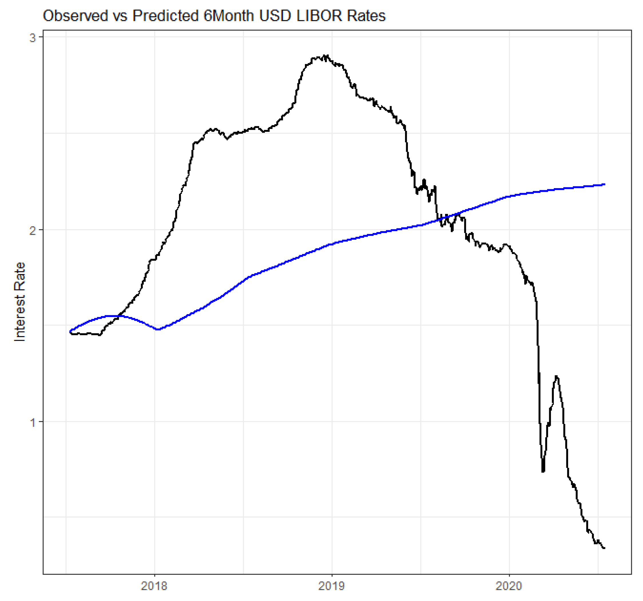
• Model Calibration: In order to calibrate the Hull–White one-factor model, both the term structure of spot rates and implied volatilities are required. Unlike some other interest rate models, which uses historical series data to calculate parameters, the Hull–White model utilizes cross-sectional data from a single point in time Kladívko and Rusý (2023) to calibrate the model. For our calibration, we utilized LIBOR spot rates with various tenors (1D, 1W, 1M, 2M, 3M, and 6M) on July 7, 2017, as well as ICE Swap rates with tenors (1Y, 2Y, 3Y, 4Y, 5Y, 6Y, 7Y, 8Y, 9Y, 10Y, and 15Y) to obtain the full term structure of interest rates for that date ICE Benchmark Administration (2023). Normally, implied volatilities for 7 July 2017 would be obtained using interest rate derivatives such as swaptions. However, since we lack access to these data, we derived historical volatilities from forward rate curves constructed using daily ICE Swap rate curves from 14 August 2014 to 7 July 2017. These historical volatilities were used in place of implied volatilities. The parameter $\alpha$ in Equation (8) was established as $0.0001$, based on the values in Table 5 for 2014, 2015, and 2016 in Kladívko and Rusý (2023).
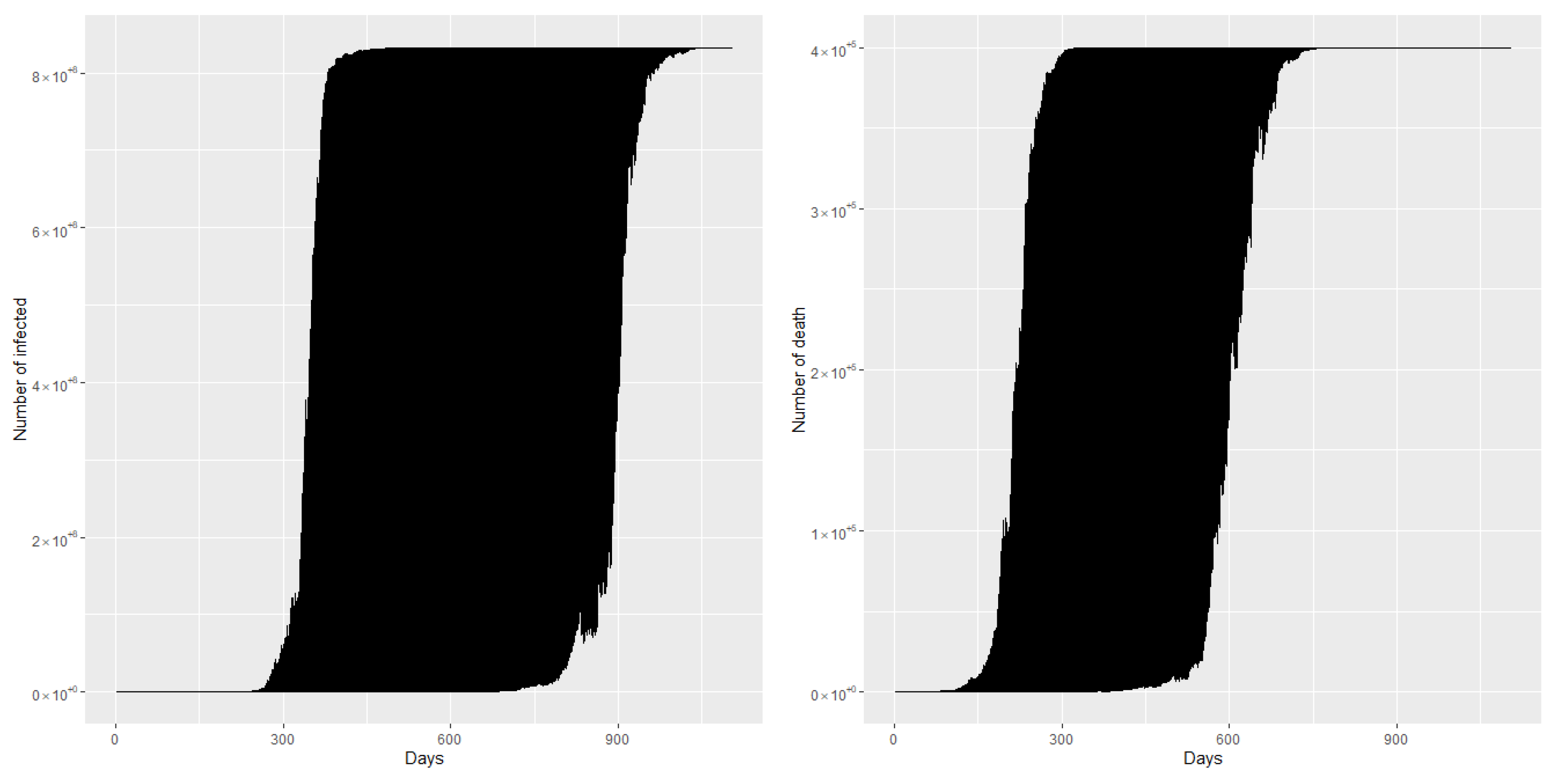
• Simulation: Post-calibration, the model is employed to simulate short rates (instantaneous interest rates at specific points in time) 5000 times within the designated time interval. Our focus lies on the 6-month USD LIBOR rates. For each simulated short rate path, we can obtain the short rate values for the subsequent 6 months and compute the average rate during that period. This average rate can be called as the approximated 6M USD LIBOR rate for that particular date within that path. Since we possess 5000 such rates for that date (derived from 5000 sample paths), we once again calculate the average. This average is considered as the 6M USD LIBOR rate for that date, utilized for subsequent computations. When simulating paths, we assumed that an year is 252 days (trading days) and used 126 days for 6 months.

The simulated Hull–White short-rate curves are given in Figure 1. Since the Hull–White model uses normal distribution, negative rates are possible.

The predicted 6M USD LIBOR curve on 7 July 2017 and later observed real 6M USD LIBOR curve are given in Figure 2. The prediction was made on 7 July 2017 based on the Hull–White model.

Once 6M USD LIBOR rates are obtained, nth coupon of the bond, $F{r}_n$, can be calculated as follows:

$$F{r}_n=225M\times \left(\frac{r_{n-1}+6.5\%}{100}\right)\times \left(\frac{d_n}{360}\right)$$

(31)

where $225M$ is the face value, $r_{n-1}$ is the predicted 6M USD LIBOR rates on $(n-1)$th coupon date, $6.5\%$ is the spread, and $d_n$ is the actual number of days between $(n-1)$th and nth coupon payment dates. The issue price of World Bank pandemic bond is 100%. Additionally, the 6M USD LIBOR rate on 7 July 2017 was 1.46544%. Therefore, investors knew the amount of first coupon payment (to be paid on 15 August 2017) at issue (on 7 July 2017). Only uncertainties were what would be the remaining future coupon payment amount (based on future 6M LIBOR rates) and whether the trigger of the bond will be activated or not before the maturity. These two uncertainties were evaluated by each investor according to their own risk preferences. The exact coupon amount, exact LIBOR rates used for that calculation and the exact coupon payment date for the World Bank pandemic bond are not easy to find. We requested these data from the World Bank and are yet to receive exact values. Therefore, based on the bond prospect, we created a

Table 3. Most likely real coupon paid date, real coupon amounts, referenced LIBOR rates, predicted LIBOR rates, and the predicted coupon amount without COVID-19 effect.

	Date	Real 6M.LIBOR	Real.Coupon (USD Million)	Predicted 6M.LIBOR	Pred.Coupon (USD Million)
	2017-07-07	1.40000	NA	NA	NA
1	2017-08-15	1.45333	1.941576	1.514160	1.941576
2	2017-09-15	1.47111	1.540958	1.541704	1.552743
3	2017-10-16	1.53316	1.544403	1.547542	1.558080
4	2017-11-15	1.61810	1.506217	1.534158	1.508914
5	2017-12-15	1.77443	1.522144	1.501944	1.506405
6	2018-01-15	1.89875	1.603171	1.481613	1.550377
7	2018-02-15	2.09644	1.627258	1.519304	1.546438
8	2018-03-15	2.34175	1.504377	1.556905	1.403378
9	2018-04-16	2.50313	1.768350	1.598791	1.611381
10	2018-05-15	2.49250	1.631817	1.644671	1.467906
11	2018-06-15	2.50375	1.742297	1.700423	1.578030
12	2018-07-16	2.51850	1.744477	1.751601	1.588832
13	2018-08-15	2.51063	1.690969	1.783887	1.547175
14	2018-09-17	2.57075	1.858442	1.815619	1.708552
15	2018-10-15	2.65375	1.587381	1.844416	1.455233
16	2018-11-15	2.86019	1.773539	1.877727	1.616731
17	2018-12-17	2.90463	1.872038	1.909304	1.675545
18	2019-01-15	2.84581	1.704589	1.931655	1.524186
19	2019-02-15	2.75375	1.810751	1.950721	1.633633
20	2019-03-15	2.67175	1.619406	1.966666	1.478876
21	2019-04-15	2.63763	1.777027	1.982977	1.640417
22	2019-05-15	2.55088	1.713306	1.996944	1.590558
23	2019-06-17	2.30875	1.866744	2.012034	1.752495
24	2019-07-15	2.21713	1.541531	2.027451	1.489606
25	2019-08-15	2.01400	1.688944	2.054883	1.652194
26	2019-09-16	2.07800	1.702800	2.080081	1.710977
27	2019-10-15	1.97725	1.554763	2.105046	1.555140
28	2019-11-15	1.91850	1.642467	2.132781	1.667228
29	2019-12-16	1.89338	1.631084	2.157987	1.672601
30	2020-01-15	1.86500	1.573759	2.176524	1.623373
31	2020-02-17	1.72488	1.725281	2.189160	1.789533
32	2020-03-16	0.84375	1.439354	2.199016	1.520603
33	2020-04-15	1.15013	1.376953	2.207977	1.631066
34	2020-05-15	0.65900	1.434399	2.216058	1.632746
35	2020-06-15	0.43088	1.387056	2.223039	1.688736
36	2020-07-15	NA	1.299540	NA	1.635570
	2017-07-07	real yield (no COVID): 8.8978%		pred. yield (no COVID): 8.6734%

, which contains the most likely coupon payment dates, most likely real 6M LIBOR rates used (based on daily 6M LIBOR rates provided by ICE Benchmark Administration (2023)) to calculate the coupon payment, most likely real coupon payment amount, predicted LIBOR rates(under the Hull–White model on 7 July 2017), and the predicted coupon amount.

If we assume the bond will not be triggered, then based on the predicted future coupon payments in Table 3, we can calculate the yield to maturity for this bond using Equation (32).

$$\begin{array}{c}225M=\sum _{n=1}^{36}\frac{F{r}_n}{{(1+y)}^{\frac{t_n}{360}}}+\frac{225M}{{(1+y)}^{\frac{1104}{360}}}\hfill \end{array}$$

(32)

There are 36 coupon payments dates between 7 July 2017 and 15 July 2020 starting 15 August 2017 and 1104 days including the start date. Here, the first coupon payment amount $F{r}_1$ on 15 August 2017 is known at the purchase date (7 July 2017 ), the remaining coupons, $\left\{F{r}_n\right\}{}_{n=2}^{36}$ are unknown and should be calculated using Equation (31), y is the effective annual yield to maturity, and $t_n$ is the number of days between 7 July 2017 and the nth coupon payment date. The first coupon payment can be calculated as

$$F{r}_1=225M\times \left(\frac{1.46544+6.5}{100}\right)\times \frac{39}{360}\approx 1.94M$$

The World bank use the actual/360 system, and there are 39 days in between 7 July 2017 and 15 August 2017 including the start date. The yield rate calculated using the predicted coupon amounts given in Table 3 and Equation (32) is $8.6734\%$. This yield rate can be considered as the investor’s expected annual return rate (or internal rate of return) for this investment. We also calculated what would have been realized if no COVID-19 had occurred and if investors received all coupon payments based on real 6M LIBOR rates. This value is $8.8978\%$. We would like to mention that these two yield rates are very close, which validate the simulation of the 6M LIBOR curve based on the Hull–White model.

Next we calculate what the investor is willing to pay for the bond, if the investor still expects the same annual return rate, but accounts the pandemic into the pricing through our proposed model. Calculation of this value is a little bit different from the bond price given in Equation (18). In that equation, the discounting process is based on the short rate models. But here the discounting factor is fixed, since the investor knows the required yield rate as y, which we calculated as $8.6734\%$. Therefore, this price is not the fair value of the pandemic bond, but the price that the investor is willing to pay to match to have same return rate for pandemic bonds when no pandemic occur. The pricing formula is still close to Equation (18).

$$\begin{array}{cc}E\left[\mathrm{Bond}\mathrm{Price}\right]\hfill & =E\left[\mathrm{Bond}\mathrm{Price}\right|\mathrm{Trigger}\left]P\right(\mathrm{Trigger})\hfill \\ \hfill & +E\left[\mathrm{Bond}\mathrm{Price}\right|\mathrm{No}\mathrm{Trigger}\left]P\right(\mathrm{No}\mathrm{Trigger})\hfill \\ \hfill & =E\left[\sum _{n=1}^m\frac{F{r}_n}{{(1+y)}^{\frac{t_n}{360}}}|\mathrm{Trigger}\right]P\left(\mathrm{Trigger}\right)\hfill \\ \hfill & +E\left[\frac{M}{{(1+y)}^{\frac{t_{36}}{360}}}+\sum _{n=1}^{36}\frac{F{r}_n}{{(1+y)}^{\frac{t_n}{360}}}|\mathrm{No}\mathrm{Trigger}\right]P\left(\mathrm{No}\mathrm{Trigger}\right)\hfill \\ \hfill & =E\left[\sum _{n=1}^m\frac{F{r}_n}{{(1+y)}^{\frac{t_n}{360}}}|C\right]{\mathbb{P}}_2\left(C\right)\hfill \\ \hfill & +E\left[\frac{M}{{(1+y)}^{\frac{t_{36}}{360}}}+\sum _{n=1}^{36}\frac{F{r}_n}{{(1+y)}^{\frac{t_n}{360}}}|C^{\prime }\right]{\mathbb{P}}_2\left(C^{\prime }\right),\hfill \end{array}$$

(33)

where $F{r}_n$ denotes the nth coupon amount, m denotes the number of coupons to be received if trigger event occur (uncertain), $t_n$ denotes number of days between 7 July 2017 and nth coupon payment date, M denotes redemption amount, events $C,C^{\prime },{\mathbb{P}}_2\left(C\right)$, and ${\mathbb{P}}_2\left(C^{\prime }\right)$ are defined and calculated in Equation (15). The net present value (NPV) of the investment under various interest rates given in Figure 3. NPV is a good indicator to determine whether one should invest in that project or not. Figure 3 shows that if the required yield rate is less than 8.67% (from Table 3), then the net present value of entire future cashflows is positive. Given that the effective interest rate in the market was less than 2% at the time (during 2017), this is a very attractive investment for any investor.

7.2. Probability of a Pandemic Event

In order to obtain the probability of the occurrence of a pandemic event during the bond term, given that there was no pandemic at the time of issue, we used historical data. Thirteen pandemics were reported in Patterson (1986). These pandemics occurred in the following years: 1729, 1732, 1781, 1788, 1830, 1833, 1836, 1889, 1899, 1918, 1957, 1968, and 1977 (see Table 5.1 in Patterson (1986)). We can also add well-known SARS (2003) (World Health Organization 2015), H1N1 Swine Flu (2009), and West African Ebola (2014), to this list. We cannot add COVID-19 (2019), since we are pricing a bond on 7 July 2017. We use the first recorded year as the beginning year of the pandemic in our calculation. Therefore, the interpandemic time can be listed as $3,49,7,42,3,3,53,10,19,39,11,9,26,3$, and 5. The bond we discuss in this section is issued in the year 2017. Thus, we have three years of censored observation from 2014 (from Ebola) to 2017, which we denoted as $3+$. We calculate the parameters of the Weibull distribution using Equation (16) and the maximum likelihood estimation method. We used the R package Rfast2 (R Core Team 2022) and the function censWeibull.mle for this purpose. The calculated parameters are $\tau =1.0578$, and $\theta =19.4242$. The QQ plot for the fitted distribution vs data is given in Figure 4. The QQ plot shows that the Weibull distribution fits to the data set somewhat closely. The p-value of the Kolmogorov–Smirnov test is 0.524, which indicates that there is no difference between the empirical data distribution and the fitted Weibull distribution.

Next we calculate the probability of a pandemic during the bond term from Equation (17),

$$\begin{array}{cc}P\left(H\right)\hfill & =\frac{{\mathbb{P}}_2(X>2017-2014)-{\mathbb{P}}_2(X>2017+3-2014)}{{\mathbb{P}}_2(X>2017-2014)}=0.1393\mathrm{and}\hfill \end{array}$$

(34)

$$\begin{array}{cc}P\left(H^{\prime }\right)\hfill & =1-P\left(H\right)=0.8607.\hfill \end{array}$$

(35)

At this point one may ask what would be the predicted probability, if the exponential distribution is used instead of the Weibull distribution. We fitted the exponential distribution to the data set using the maximum likelihood method for comparison purposes. The KS statistics is 0.6407 indicating that the exponential distribution fits well to the data same as the Weibull distribution. The predicted probability was 0.1461 compared to 0.1393 above. Therefore, if exponential distribution is used, it would result in lower bond price than when used by the Weibull distribution. Although both distributions fit well to inter-pandemic time, predict somewhat closer probability of pandemic, we continue with the Weibull distribution, mainly due to novelty in application.

7.3. Trigger Event

We have defined the trigger event as the seven-day moving average for daily new death, $m{a}_D\left(t\right)$ exceeding ${\theta }_D$, the seven-day running average for the daily number of infected, $m{a}_I\left(t\right)$, exceeding ${\theta }_I$ and the infection growth rate, and $GR\left(t\right)$ being positive before the maturity of the bond. All events should occur at the same time t to activate the trigger. The number of infected and number of deaths simulated using the stochastic logistic growth model. Once we have the cumulative number of infections and deaths from the logistic model, we can calculate $m{a}_D\left(t\right),m{a}_I\left(t\right)$, and $GR\left(t\right)$. Based on the World Bank operation manual and the bond prospectus (World Bank 2017b, 2018), we used the following as our threshold values in this research.

$${\theta }_I=5000\mathrm{infections}\mathrm{per}\mathrm{seven}\mathrm{day},\mathrm{and}{\theta }_D=2500\mathrm{deaths}\mathrm{per}\mathrm{seven}\mathrm{day}$$

(36)

The bond, we are trying to price is issued on 7 July 2017. COVID-19 had not yet occurred, and most investors may not have suspected a pandemic within the next three years. Therefore, we will price the bond under past four influenza pandemic scenarios, and calculate the average price. These are 1918-“Spanish flu”, 1957-“Asian flu”, 1968-“Hong Kong flu”, and 2009-“Swine flu”. In order to use the model described above in each scenario, one needs $I\left(0\right),D\left(0\right),K_I,K_D,g_I,g_D,{\sigma }_I$, and ${\sigma }_D$. We will use the following table to estimate these parameters.

Data for first four columns of this table was obtained from World Health Organization (2013). The reproduction number, ${\mathcal{R}}_0$, measures “the average number of secondary cases of disease caused by a single infected individual over his or her infectious period” (Cori et al. 2013). If ${\mathcal{R}}_0<1$, it is expected that the outbreak will subdue very soon and conversely, if ${\mathcal{R}}_0>1$, then the outbreak may grow relatively quickly and become an epidemic. The case fatality rate (CFR) in the context of an epidemic refers to the proportion of deaths among individuals who have been diagnosed with the disease. It is calculated by dividing the number of deaths caused by the disease by the number of confirmed cases and multiplying the result by 100 to express it as a percentage. The CFR for the 1918, 1957, and 1968 pandemics was obtained from (Li et al. 2008). CFR for the 2009 pandemic was obtained from (Nishiura 2010). The references for the average infectious period are from (Bajardi et al. 2011; Jackson et al. 2010; Mills et al. 2004; Vynnycky and Edmunds 2008). The connection between the growth rate, g, used in the logistic model, and the number of reproductions, ${\mathcal{R}}_0$, was investigated in (Ma 2020). Under SIR compartment model, the relationship can be written as,

$$g=\gamma ({\mathcal{R}}_0-1).$$

(37)

Here, $1/\gamma$ is the average infectious period. We use Equation (37) to calculate the growth rates in the seventh column of

Table 4. Characteristics of the past four influenza pandemics.

Year	Virus Type	Estimated Reproduction Number (${\mathcal{R}}_0$)	Estimated Total Death	Case Fatality Rate (%)	Average Infectious Period ($1/\mathit{\gamma }$)	Growth Rate for Infection (${\mathit{g}}_{\mathit{I}}$)	Estimated Total Infections
1918	H1N1	1.2–3.0	20–50 M	2.5	4.1 days	0.049–0.488	800–2000 M
1957	H2N1	1.5	1–4 M	0.1–0.4	4 days	0.125	1000 M
1968	H3N2	1.3–1.6	1–4 M	0.1–0.4	4 days	0.075–0.150	1000 M
2009	H1N1	1.1–1.8	0.1–0.4 M	0.048	2.5 days	0.040–0.320	208–833 M

. The last column was calculated using the columns “Case Fatality Rate” and “Estimated Total Death”. Before we continue, we would like to emphasize the difficulty in obtaining reliable data for a historic pandemic. Therefore, it is possible that the data represented in Table 4 may overestimate or underestimate the true values. For example, Table 4 indicate that the maximum total infection for the 1918 Spanish flu pandemic should be around 2000 M, but the world population at that time was close to 1800 M.

In each scenario, the carrying capacity for deaths and infections $K_D,K_I$ is set using values in the columns “Estimated total death” and “Estimated total infection” (either lower bound or upper bound) of Table 4. The initial number of infections for $I\left(0\right),D\left(0\right)$ set at 1. Since there is no reproduction number defined for deaths, we used the same growth rate for $g_I$ and $g_D$. Volatility terms, ${\sigma }_I,{\sigma }_D$ are set ad hoc, which can be based on historical records or expert opinion. The correlation coefficient between the number of infected and death is set at $0.5$. The algorithm to calculate the price of the bond under the 2009 H1N1 Influenza pandemic scenario is given in Algorithm 1.

Algorithm 1 The algorithm to calculate bond price under the 2009 H1N1 Influenza pandemic scenario
Require:  Predicted bond coupon payments $F{r}_n$	▹ see Section 7.1 and Table 3
Require:  Investors expected annual return rate y (calculated as 8.2837%)	▹ see
Equation (32)
$I\left(0\right)\leftarrow 1$
$D\left(0\right)\leftarrow 1$
$K_I\leftarrow 833M$	▹ see Table 4
$K_D\leftarrow 0.4M$	▹ see Table 4
$g_I\leftarrow 0.320$	▹ see Table 4
$g_D\leftarrow g_I$	▹ we set both rates to be same, since it is not possible to calculate $g_D$ without
real data
${\sigma }_I,{\sigma }_D\leftarrow 0.1$	▹ we set both rates to be same
$dt\leftarrow 1$	▹ time step of the simulation is set to 1 day
$N\leftarrow 1104$	▹ Number of steps. This is the number of days between 7 July 2017–15 July 2020.
${\theta }_I\leftarrow 5000$	▹ This is the trigger for number of infected
${\theta }_D\leftarrow 2500$	▹ This is the trigger for number of death
$\rho \leftarrow 0.5$	▹ $I\left(t\right)$ and $D\left(t\right)$ are correlated stochastic processes. See Equation (29)
$M\leftarrow 5000$	▹ Number of simulation paths
$Trigger\leftarrow 0$	▹ Number of triggered events
$Time\leftarrow \left\{\right\}$	▹ The time, triggering event occurred, place holder
$BondValuePartial\leftarrow \left\{\right\}$	▹ Price of the pandemic bond(triggered), place holder
$B{V}_{full}\leftarrow 225M$	▹ the price of the bond investor willing to pay if no pandemic occur.
This is the selling price of World Bank pandemic bond
$P\left(H\right)\leftarrow 0.1393$	▹ probability of Pandemic. See Equation (34)
for$i=1$ to M do
Simulate solution to stochastic differential equations with time step size $dt$ and number of steps N. $$\begin{array}{cc}dI\left(t\right)\hfill & =I\left(t\right)\left(1-\frac{I\left(t\right)}{K_I}\right)\left(g_{I}dt+{\sigma }_{I}d{B}_I\left(t\right)\right),\hfill \\ dD\left(t\right)\hfill & =D\left(t\right)\left(1-\frac{D\left(t\right)}{K_D}\right)\left(g_{D}dt+{\sigma }_{D}d{B}_D\left(t\right)\right),\\ d{B}_I\left(t\right)\hfill & =d{W}_1\left(t\right),\hfill \\ d{B}_D\left(t\right)\hfill & =\rho d{W}_1\left(t\right)+\sqrt{1-{\rho }^2}d{W}_2\left(t\right)\hfill \end{array}$$      Solution paths are $I\left(t\right)$ and $D\left(t\right)$      Calculate daily increments using $max(0,I(t)-I(t-1\left)\right)$ and $max(0,D(t)-D(t-1\left)\right)$      Starting day 7 to day 1104, calculate past seven day average for daily new infections and deaths.
Seven day average paths are $m{a}_I\left(t\right),m{a}_D\left(t\right)$	▹ see Section 5.2.2
Calculate standard deviation of past seven day daily new infections
Calculate growth rate $GR\left(t\right)$	▹ see Equation (6)
if $(m{a}_D\left(t\right)>{\theta }_D)\&(m{a}_I\left(t\right)>{\theta }_I)\&(GR\left(t\right)>0)$ then
$Trigger\leftarrow Trigger+1$
$Time<-Append(Time,t)$	▹ Add time of the trigger event to the set
$B{V}_{partial}\leftarrow$ Bond Value based on coupons paid until time t	▹ see Equation (33)
$BondValuePartial\leftarrow Append(BondValuePartial,B{V}_{partial})$
end if
end for
$E\left[BondPrice\right|Trigger]\leftarrow$ average of values in $BondValuePartial$ set
$E\left[BondPrice\right|NoTrigger]\leftarrow B{V}_{full}$
$P\left(C\right)\leftarrow (Trigger/M)P\left(H\right)$	▹ P(H) from above. See Equation (15)
$P\left(C^{\prime }\right)\leftarrow 1-P\left(C\right)$
$BondPrice\leftarrow E\left[BondPrice\right|Trigger]P\left(C\right)+E\left[BondPrice\right|NoTrigger]P\left(C^{\prime }\right)$

The algorithm was implemented in Rlgorithm was implemented in R and can be found in the Manathunga (2023). The graphs of the simulated paths under 2009 H1N1 influenza pandemic is given in Figure 5.

We simulated 5000 sample paths for each of above mentioned pandemic scenarios and calculated bond price. We used the parameters listed in Algorithm 1, except for $K_I,K_D$ and $g_I$. The parameters used, the calculated bond value, and the probability of trigger being activated are given in

Table 5. The World Bank issued pandemic bond, priced under each historic pandemic if required yield rate is 8.6734%.

Scenario	Spanish Flu (1918)	Asian Flu (1957)	HongKong Flu (1968)	Swine Flu (2009)
$K_I$	2000 M	1000 M	1000 M	833 M
$K_D$	50 M	4 M	4 M	0.4 M
$g_I$	0.049	0.125	0.075	0.04
Bond Price	195.5866	194.2548	194.8468	201.4460 M
$P\left(C\right)$	0.1392	0.1393	0.1391	0.1132
Average price: 196.5335

.

According to the data presented in Table 5, it can be observed that in order to achieve the same yield rate as one would receive under a no pandemic scenario, investors should have paid USD 196.53 million instead of USD 225 million. One of the key parameters we set in the Algorithm 1 is the volatility parameter ${\sigma }_I$ and ${\sigma }_D$. We investigate the behavior of volatility and bond price under the 2009 H1N1 pandemic. We assume that the investor still requires the yield of 8.6734%, use the coupon payments predicted in Table 3 and account pandemic through the logistic growth model. The parameters used in the simulation are the same as the parameters in Table 5 and Algorithm 1 except for ${\sigma }_I,{\sigma }_D$.

Table 6. The bond price movement against volatility terms.

${\mathit{\sigma }}_{\mathit{I}},{\mathit{\sigma }}_{\mathit{D}}$	0.04	0.08	0.12	0.16	0.20	0.24	0.28	0.32	0.36	0.40
Bond.Price	195.70	198.92	203.54	207.80	212.93	220.20	224.46	224.99	225.00	225.00
Prob.Trigger	0.14	0.12	0.10	0.08	0.06	0.02	0.00	0.00	0.00	0.00

suggests that as the volatility of the number of deaths and the number of infected increases, the probability of activation of the trigger becomes smaller. Hence the bond price come close to the no-trigger price of the bond (USD 225M).

8. Numerical Simulation 2

In this section, we calculate the fair price of a three year coupon bond under our model. To simulate the price, we need parameters for the pandemic bond, the interest rate model, the probability of the pandemic event, and if the pandemic occurs, then the probability of the trigger being activated. The R code for this simulation can be found in Manathunga (2023). The major differences of this numerical example and the previous example are the following:

• The investor want to know the fair price based on future interest rate movements, opposed to setting fixed required yield rate.
• Some model parameters are calibrated using COVID-19 data. Most other past pandemics do not have day to day records of number of infections, death, etc. But COVID-19 may be the first pandemic where humans were able to record day-to-day statistics. Therefore, the model can be calibrated using daily data instead of using aggregate numbers.

8.1. Bond Parameters

We assume that the bond was issued on 7 January 2023, for a three-year term. We also assume that there is no pandemic at the moment (assuming COVID-19 is in endemic stage now). The bond pays floating coupons at a rate of 6 month USD LIBOR + 6.5%. We also assume that LIBOR rate reset dates are coupon payment dates. If a pandemic occurs before the maturity date and the trigger is activated, then the investor will lose the full principal amount and the remaining coupons. We also assume that the investor will use COVID-19 data and the model proposed in this article to calculate the price of the bond. The chosen values of the bond parameter for this demonstration are given in

Table 7. Bond parameters for numerical simulation 2.

Parameter	Value
Settle Date	6 January 2023
Maturity Date	15 January 2026
Term	3 years
M	USD 225M
Coupons	6 month USD LIBOR + 6.5%
Payment Date	15th day of each month including 15 February 2023 to 15 January 2026
Day convention	Actual/360
Hull–White Model	Calibrated to 6 January 2023
Stochastic-logistic growth model	Calibrated using COVID-19 data
${\theta }_I$	5000
${\theta }_D$	2500

.

8.2. Interest Rate Model Parameters

Next, we generate 5000 sample paths of interest rates under the Hull–White short rate model to simulate 6M LIBOR rates and discount factors. The process of calibrating the model and the calculating bond coupons is similar to what we explained in the previous example. The model is calibrated to 6 January 2023 market data. In order to calculate the price of the bond considering the future evolution of interest rates under the Hull–White model, it is necessary to have discount rates. This is different from the previous example, where we used a fixed yield rate to discount cash flows. The simulated discount rate paths, the average discount rate curve and the predicted 6M USD LIBOR rate curve are given in Figure 6.

8.3. Calculating Probability of a Pandemic Event and Estimating Parameters for $I\left(t\right)$ and $D\left(t\right)$

To calculate the probability of a pandemic event, we used the same approach as earlier. But now we can add 2019 COVID as an pandemic event and 4+ censored observation (from 2019 to 2023) in to the data set used in Section 7.2. The new data set (inter arrival times between pandemics) is: 3, 49, 7, 42, 3, 3, 53, 10, 19, 39, 11, 9, 26, 3, 5, 5, and 4+. The new probability of a pandemic, $P\left(H\right)$, is given in

Table 8. Numeric example 2: The fair value of the bond price under proposed model.

Scenario	I	II	III
# Simulations	5000	5000	5000
$K_I$	100.46 M	100.46 M	100.46 M
$K_D$	1.1 M	1.1 M	1.1 M
$I\left(0\right)$	1	1	1
$D\left(0\right)$	1	1	1
$g_I,g_D$	0.4842	0.0147	0.2064
${\sigma }_I$	0.0521	0.0522	0.1309
${\sigma }_D$	0.0020	0.0020	0.0067
$\rho$	0.5	0.5	0.5
Bond Price	192.3830	205.3894	192.4687
$P\left(C\right)$	0.1468	0.1161	0.1468
$P\left(H\right)$	0.1468	0.1468	0.1468
Average price: USD 196.747 million

. With COVID-19, the probability of another pandemic in the next three years increased from 0.1393 to 0.1468. Next, we need values for $I\left(0\right),D\left(0\right)$, $K_I,K_D$, $g_I,g_D,{\sigma }_I$, and ${\sigma }_D$. Several model parameters were calibrated using historical COVID-19 data for the United States. Data were obtained from an R package named COVID-19 (Guidotti and Ardia 2020). The number of infections and the number of deaths due to COVID-19 in the US are given in Figure 7 which was obtained using Mathematica Wolfram Research, Inc. (2023).

We set $I\left(0\right)$ and $D\left(0\right)$ to be 1 as earlier. $K_I,K_D$ values are set to be the total number of infected and the total number of deaths as of 31 December 2022 in USA from the data set. Instead of using the reproduction number to calculate growth rates $g_I,g_D$, we use the following data-driven approach. First, we calculate daily growth rates, $g\left(t\right)$, at each time point using the following equation.

$$g\left(t\right)=\frac{N\left(t\right)-N(t-1)}{N(t-1)}.$$

(38)

A plot of daily growth rates for the number of infections and the number of deaths given in Figure 8. Note that two growth rates have different maximum. Therefore, we should set $g_I,g_D$ separately instead of the same value. But this was not possible with the method we employed in the numerical example 1.

So, what should be g? There is no definitive answer. But here are a few approaches that one can use:

• Calculate the maximum. This gives $g_I^{max}=0.4842$ and $g_D^{max}=0.0385$.
• Calculate the average of nonzero growth rates. This gives $g_I^{avg}=0.0147$ and $g_D^{avg}=0.0004$.
• Calculate the average of growth rates up to certain date such as right before the growth rates become close to zero. If we use first the 50 days, then $g_I^{50}=0.2064$ and $g_D^{50}=0.0065$.
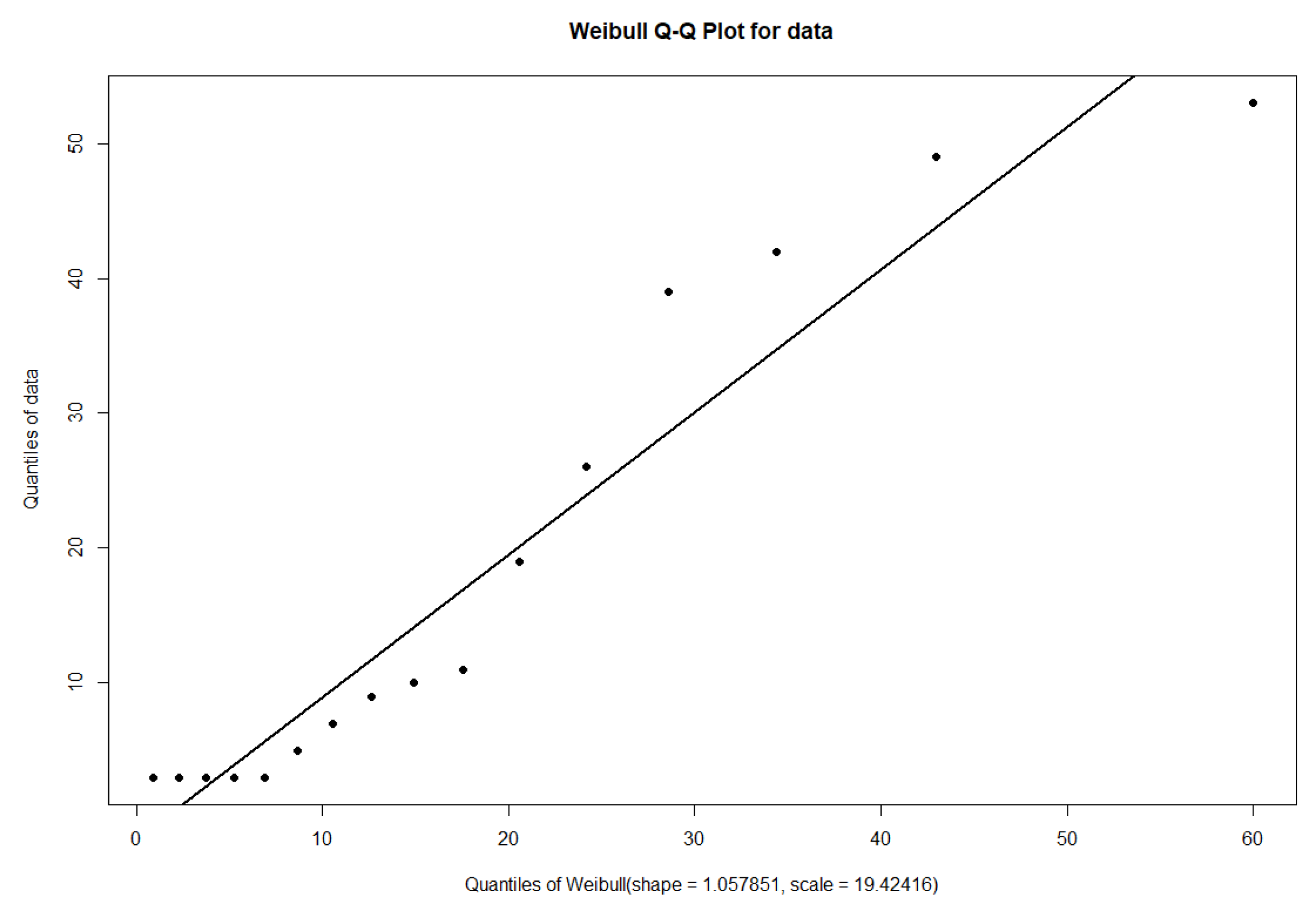
• Fit a parametric distribution such as log normal or gamma and use statistics such as mean or median of the fitted distribution as the growth rate.

However, we have observed that when $g_I$ and $g_D$ are too far away from each other, there would be a delay between the number of infection curves and the number of death curves, which would affect the trigger event and not natural (the delay is more than the average infectious period). Therefore, we again set both values at the same level. Volatility terms ${\sigma }_I,{\sigma }_D$ are calculated as standard deviations of the growth rates and set separately. The correlation coefficient was set to 0.5 as in the previous example. At this point, one may wonder what would be the growth rate, if we used the reproduction number, ${\mathcal{R}}_0$, and the average infectious period to calculate it using Equation (37). The average infectious period for COVID-19 is 5.1 days (Lauer et al. 2020) and the reproduction number of COVID-19 Liu et al. (2020) is 3.28. These values infer the growth rate of the infection to be 0.447. The calculated bond price and parameters are given in Table 8.

Finally we evaluate the bond under the parameter grid given in

Table 9. Numerical example 2: average pandemic bond price under various parameter combinations.

$g_I$	0.1, 0.2, 0.3, 0.4
$g_D$	0.1, 0.2, 0.3, 0.4
$s_I$	0.02, 0.04, 0.06, 0.08, 0.10, 0.12, 0.14, 0.16, 0.18, 0.20
$s_D$	0.02, 0.04, 0.06, 0.08, 0.10, 0.12, 0.14, 0.16, 0.18, 0.20
$rho$	0.1, 0.2, 0.3, 0.4, 0.5, 0.6, 0.7, 0.8, 0.9
# of parameter combinations	14,400
# Simulations	each combination 100 times
Average bond price under this grid	USD 205.3762 million
Average probability for trigger activation	0.0887

. Under this approach, we consider all possible combinations of parameters. When we calculated the price of bond given in numerical example 2, we found USD 205.3762 million as the price. This is again close to price we received earlier (USD 196 million). Each combination was simulated 100 times. There are 14,400 possible combinations, which resulted 1.44 million total simulations.

9. Discussion

A pandemic is one of the most devastating disasters that can occur to humankind. The recent COVID-19 pandemic shows that a pandemic can have a profound impact on all aspects of human life. Pandemic bonds can be used by the government to mitigate financial losses and rapidly fund pandemic-related activities such as vaccine programs, buying hospital equipment, etc. Up to now, almost all pricing mechanisms of pandemic bond studies have relied on compartmental models such as SIR or its variants, including pandemic bonds issued by the World Bank, which used the AIR Worldwide developed compartment model. Our study performed the following:

• We proposed a pandemic bond pricing framework based on the stochastic logistic model and the Hull–White interest rate model.
• We review the details of the World Bank-issued pandemic bond.
• We used past four influenza pandemics to price World Bank issued pandemic bond, and hence demonstrating how to use the model when aggregate information of past pandemics is available. Even though we used information from four pandemics, the example shows how to use all available past pandemic scenarios in the modeling process.
• We used COVID-19 data to calibrate the model parameters using a data-driven approach and price a pandemic bond. Therefore, we demonstrate how to use the model when detailed data are available. The purpose of using COVID-19 data is not to claim that future pandemics would be look like COVID -19 but to demonstrate a data-driven approach.
• We showed how to use a parameter grid to remove any restrictions for $g_I,g_D,{\sigma }_i,{\sigma }_D,\rho$ and calculate across all possible combinations to obtain the fair price of a pandemic bond.
• We calculate the price of the bond under two different scenarios. First, when an investor knows the required yield, find the price he/she is willing to pay. Second, the fair price of the pandemic bond under the model.
• We created an algorithm to implement the model and made R codes and other data sets available for future research/testing and reproducibility.

We also used the Weibull distribution to calculate the probability of a pandemic during the bond term, thus deviating from popular memory-less distributions. We simplified some pandemic bond trigger criteria from the World Bank and numerically demonstrated how to implement the model, giving potential investors a more transparent pricing mechanism. The model can be easily calibrated to any data set and the price can be obtained using simulation techniques. The study shows that if investors considered the pandemic, then they should have paid 196.53/225 = 87% of the issue price for the pandemic bond issued by the World Bank instead of 100%. Even after taking COVID-19, the fair price of similar-type bonds still close to the same price, with the exact price given as USD 196.75 million. We also observed that when volatility of number of infection and number of death increase, the price of bond close to the face value. Another observation coming from this model is that when setting parameter values, expert opinion may be required. For example, the correlation value between two stochastic processes, growth rates, and volatility of growth terms may require some expert opinion before using in the model even though we used past data without any corrections. This is typical in any real world scenario modeling, where the modeler has to decide the parameter values.

We also identify some limitations in this study. First, we assumed that the interest rate process is independent from the occurrence of pandemic event. This is not true in the real world, as we have seen in the US stock market reaction to COVID 19 on 16 March 2020. However, the market recovered rapidly than experts expected before inflation settled in. Regardless of which interest rate model use, it would be hard to capture all the nitty-gritty details of the market in the model. However, adding dependent interest rate process is one improvement one can make to this model. Second, we assumed that the number of infections and deaths are correlated; therefore, we did not study this relationship in full detail and most of the time we set the correlation coefficient arbitrarily at 0.5. In the real world, for example, at the onset of the pandemic, due to less understanding of the disease, there may be a very strong correlation between the number of deaths and the number of infections. As time passes, once vaccines are available with a better understanding of patient care, infection and death can become uncorrelated. We also assumed that if a pandemic occurs, it happens right after the pandemic bond issuance. A better approach would be to calculate the time to the next pandemic using the inter-pandemic time distribution (in our case, this is the Weibull distribution). Once we know the time to the next pandemic, from that point on, we can generate the $I\left(t\right)$ and $D\left(t\right)$ and check whether this would lead to trigger activation before the bond maturity. However, given that the pandemic bond term is typically short (three years), we can ignore the time delay. We also used constant population growth rate and volatility terms in the stochastic logistic growth model. This can be changed by fitting time-dependent $g\left(t\right)$ and ${\sigma }_N\left(t\right)$ functions.

10. Conclusions

CAT bonds or catastrophic bonds have emerged as a tool to hedge financial losses due to extreme events. CAT bonds provide financial protection by transferring financial risk to investors who are willing and able to take the risk. Investors willing to take the risk would be rewarded with a higher return as long as no catastrophe occurs during the term of the bond. Governments, reinsurers, and other corporations receive protection since they could transfer the risk from their balance sheet to investors with no credit risk. With COVID, financial losses due to pandemics became significant in many countries, thus warranting a risk transferring mechanism. This study proposes a pricing mechanism for catastrophic bonds for pandemics using the stochastic logistic growth model. Compared to some CAT bonds, such as hurricanes and earthquakes, pandemic bonds have received less attention from industry professionals, such as actuaries and academia. We hope that this research will bring more attention to the topic.

References

1. Bajardi, Paolo, Chiara Poletto, Jose J. Ramasco, Michele Tizzoni, Vittoria Colizza, and Alessandro Vespignani. 2011. Human mobility networks, travel restrictions, and the global spread of 2009 h1n1 pandemic. PLoS ONE 6: e16591. [Google Scholar] [CrossRef] [PubMed]
2. Bevere, Lucia, and Michael Gloor. 2020. Natural catastrophes in times of economic accumulation and climate change. Sigma 2: 1–36, Swiss Re Institute. Available online: https://www.swissre.com/dam/jcr:85598d6e-b5b5-4d4b-971e-5fc9eee143fb/sigma-2-2020-en.pdf (accessed on 2 October 2022).
3. Bickis, Mikelis, and Ugis Bickis. 2007. Predicting the next pandemic: An exercise in imprecise hazards. Paper presented at the 5th International Symposium on Imprecise Probability: Theories and Applications, Prague, Czech Republic, July 6–19; Available online: https://isipta07.sipta.org/proceedings/proceedings-optimised.pdf (accessed on 2 October 2022).
4. Braun, Alexander. 2012. Determinants of the cat bond spread at issuance. Zeitschrift für Die Gesamte Versicherungswissenschaft 101: 721–36. [Google Scholar] [CrossRef]
5. Cori, Anne, Neil M. Ferguson, Christophe Fraser, and Simon Cauchemez. 2013. A new framework and software to estimate time-varying reproduction numbers during epidemics. American Journal of Epidemiology 178: 1505–12. [Google Scholar] [CrossRef]
6. Cox, John C., Jonathan E. Ingersoll Jr., and Stephen A. Ross. 1985. A theory of the term structure of interest rates. Econometrica 53: 385–408. [Google Scholar] [CrossRef]
7. Cox, Samuel H., Joseph R. Fairchild, and Hal W. Pedersen. 2000. Economic aspects of securitization of risk. ASTIN Bulletin: The Journal of the IAA 30: 157–93. [Google Scholar] [CrossRef]
8. Cox, Samuel H., and Hal W. Pedersen. 2000. Catastrophe risk bonds. North American Actuarial Journal 4: 56–82. [Google Scholar] [CrossRef]
9. Cummins, J. David. 2008. Cat bonds and other risk-linked securities: State of the market and recent developments. Risk Management and Insurance Review 11: 23–47. [Google Scholar] [CrossRef]
10. Cummins, J. David. 2012. Cat bonds and other risk-linked securities: Product design and evolution of the market. In The Geneva Reports. Geneva: The Geneva Association, pp. 39–61. [Google Scholar] [CrossRef]
11. Deng, Guoqu, Shiqiang Liu, Li Li, and Chushi Deng. 2020. Research on the pricing of global drought catastrophe bonds. Mathematical Problems in Engineering 2020: 3898191. [Google Scholar] [CrossRef]
12. Edesess, Michael. 2015. Catastrophe bonds: An important new financial instrument. Alternative Investment Analyst Review 4: 6–11. Available online: https://caia.org/sites/default/files/AIAR_Q4_2015-02_Edesses_CatBonds_0.pdf (accessed on 2 October 2022).
13. Fan, Weili, and Rogemar Mamon. 2021. A hybridized stochastic sir-vasiček model in evaluating a pandemic emergency financing facility. IEEE Transactions on Computational Social Systems 10: 1105–14. [Google Scholar] [CrossRef]
14. Financial Times. 2023. After COVID-19: The Future of Pandemic Bonds. Available online: https://www.ft.com/partnercontent/calvert/after-covid-19-the-future-of-pandemic-bonds.html (accessed on 10 June 2023).
15. Guidotti, Emanuele, and David Ardia. 2020. COVID-19 data hub. Journal of Open Source Software 5: 2376. [Google Scholar] [CrossRef]
16. Gurrieri, Sébastien, Masaki Nakabayashi, and Tony Wong. 2009. Calibration Methods of Hull-White Model. Available at SSRN 1514192. [Google Scholar] [CrossRef]
17. Härdle, Wolfgang Karl, and Brenda López Cabrera. 2010. Calibrating cat bonds for mexican earthquakes. Journal of Risk and Insurance 77: 625–50. [Google Scholar] [CrossRef]
18. Huang, Shimeng, Ken Seng Tan, Jinggong Zhang, and Wenjun Zhu. 2021. Epidemic financing facilities: Pandemic bonds and endemic swaps. In Nanyang Business School Research Paper Series, Singapore, No. 21–37. [Google Scholar] [CrossRef]
19. Hull, John, and Alan White. 1990. Pricing interest-rate-derivative securities. The Review of Financial Studies 3: 573–92. [Google Scholar] [CrossRef]
20. Hull, John, and Alan White. 1993. One-factor interest-rate models and the valuation of interest-rate derivative securities. Journal of Financial and Quantitative Analysis 28: 235–54. [Google Scholar] [CrossRef]
21. Hull, John C. 2014. Options Futures and Other Derivatives. New York: Pearson Education. ISBN 978-0133456318. [Google Scholar]
22. ICE Benchmark Administration. 2023. Administering Global Benchmarks and Data Services. Available online: https://www.theice.com/iba (accessed on 15 March 2023).
23. Jackson, Charlotte, Emilia Vynnycky, and Punam Mangtani. 2010. Estimates of the transmissibility of the 1968 (hong kong) influenza pandemic: Evidence of increased transmissibility between successive waves. American Journal of Epidemiology 171: 465–78. [Google Scholar] [CrossRef]
24. Khodabin, M., Khosrow Maleknejad, M. Rostami, and M. Nouri. 2012. Interpolation solution in generalized stochastic exponential population growth model. Applied Mathematical Modelling 36: 1023–33. [Google Scholar] [CrossRef]
25. Kladívko, Kamil, and Tomáš Rusý. 2023. Maximum likelihood estimation of the hull–white model. Journal of Empirical Finance 70: 227–47. [Google Scholar] [CrossRef]
26. Klugman, Stuart A., Harry H. Panjer, and Gordon E. Willmot. 2012. Loss Models: From Data to Decisions, 4th ed. Hoboken: John Wiley & Sons. ISBN 978-1118315323. [Google Scholar]
27. Lauer, Stephen A., Kyra H. Grantz, Qifang Bi, Forrest K. Jones, Qulu Zheng, Hannah R. Meredith, Andrew S. Azman, Nicholas G. Reich, and Justin Lessler. 2020. The incubation period of coronavirus disease 2019 (COVID-19) from publicly reported confirmed cases: Estimation and application. Annals of Internal Medicine 172: 577–82. [Google Scholar] [CrossRef]
28. Lee, Jin-Ping, and Min-Teh Yu. 2002. Pricing default-risky cat bonds with moral hazard and basis risk. Journal of Risk and Insurance 69: 25–44. [Google Scholar] [CrossRef]
29. Lee, Sang-heon. 2021. Hull-White 1-Factor Model Using R Code. Available online: https://www.r-bloggers.com/2021/06/hull-white-1-factor-model-using-r-code/ (accessed on 10 March 2023).
30. Li, F. C. K., B. C. K. Choi, T. Sly, and A. W. P. Pak. 2008. Finding the real case-fatality rate of h5n1 avian influenza. Journal of Epidemiology & Community Health 62: 555–59. [Google Scholar] [CrossRef]
31. Li, Han, Haibo Liu, Qihe Tang, and Zhongyi Yuan. 2023. Pricing extreme mortality risk in the wake of the COVID-19 pandemic. Insurance: Mathematics and Economics 108: 84–106. [Google Scholar] [CrossRef] [PubMed]
32. Liu, Meng, and Ke Wang. 2013. A note on stability of stochastic logistic equation. Applied Mathematics Letters 26: 601–6. [Google Scholar] [CrossRef]
33. Liu, Ying, Albert A Gayle, Annelies Wilder-Smith, and Joacim Rocklöv. 2020. The reproductive number of COVID-19 is higher compared to sars coronavirus. Journal of Travel Medicine 27. [Google Scholar] [CrossRef]
34. Ma, Junling. 2020. Estimating epidemic exponential growth rate and basic reproduction number. Infectious Disease Modelling 5: 129–41. [Google Scholar] [CrossRef]
35. Ma, Zong-Gang, and Chao-Qun Ma. 2013. Pricing catastrophe risk bonds: A mixed approximation method. Insurance: Mathematics and Economics 52: 243–54. [Google Scholar] [CrossRef]
36. Makariou, Despoina, Pauline Barrieu, and Yining Chen. 2021. A random forest based approach for predicting spreads in the primary catastrophe bond market. Insurance: Mathematics and Economics 101: 140–62. [Google Scholar] [CrossRef]
37. Manathunga, Vajira. 2023. Pricing Pandemic Bonds under Stochastic Logistic Growth Model. Available online: https://github.com/cvajira/Pricing-Pandemic-Bonds-under-Stochastic-Logistic-Growth-Model (accessed on 21 July 2023).
38. Mills, Christina E., James M. Robins, and Marc Lipsitch. 2004. Transmissibility of 1918 pandemic influenza. Nature 432: 904–6. [Google Scholar] [CrossRef]
39. Morton N., Lane. 2018. Pricing Cat Bonds: Regressions and Machine Learning: Some Observations; Working Paper. Lane Financial LLC. Available online: http://www.lanefinancialllc.com/content/view/402/50/ (accessed on 10 March 2023).
40. Nishiura, Hiroshi. 2010. Case fatality ratio of pandemic influenza. The Lancet Infectious Diseases 10: 443–44. [Google Scholar] [CrossRef]
41. Otunuga, Olusegun Michael, and Oluwaseun Otunuga. 2022. Stochastic modeling and forecasting of COVID-19 deaths: Analysis for the fifty states in the united states. Acta Biotheoretica 70: 25. [Google Scholar] [CrossRef] [PubMed]
42. Patterson, Karl David. 1986. Pandemic Influenza, 1700–1900: A Study in Historical Epidemiology. Lanham: Rowman & Littlefield Pub Incorporated. ISBN 0847675122. [Google Scholar]
43. Privault, Nicolas. 2013. Stochastic Finance: An Introduction with Market Examples. Boca Raton: CRC Press. ISBN 978-1466594029. [Google Scholar]
44. R Core Team. 2022. R: A Language and Environment for Statistical Computing. Vienna: R Foundation for Statistical Computing. [Google Scholar]
45. Reuters. 2017. World Bank Launches ’Pandemic Bond’ to Tackle Major Outbreaks. Available online: https://www.reuters.com/article/us-global-pandemic-insurance/world-bank-launches-pandemic-bond-to-tackle-major-outbreaks-idUSKBN19J2JJ (accessed on 2 October 2022).
46. Schwarcz, Steven L. 2021. Insuring the’uninsurable’: Catastrophe bonds, pandemics, and risk securitization. Wash. UL Rev. 99: 853. [Google Scholar]
47. Shao, Jia, Apostolos D. Papaioannou, and Athanasios A. Pantelous. 2017. Pricing and simulating catastrophe risk bonds in a markov-dependent environment. Applied Mathematics and Computation 309: 68–84. [Google Scholar] [CrossRef]
48. Shen, Christopher Y. 2020. Logistic growth modelling of COVID-19 proliferation in china and its international implications. International Journal of Infectious Diseases 96: 582–89. [Google Scholar] [CrossRef]
49. Shinh, Roshni. 2021. Pandemic bonds: What Are They and How do They Work? Available online: https://actuaries.blog.gov.uk/2021/03/02/pandemic-bonds-what-are-they-and-how-do-they-work/ (accessed on 2 October 2022).
50. Swiss Re Institute. 2023. In 5 Charts: Continued High Losses from Natural Catastrophes in 2022. Available online: https://www.swissre.com/institute/research/sigma-research/sigma-2023-01/5-charts-losses-natural-catastrophes.html (accessed on 10 June 2023).
51. Triambak, S., D. P. Mahapatra, N. Mallick, and R. Sahoo. 2021. A new logistic growth model applied to COVID-19 fatality data. Epidemics 37: 100515. [Google Scholar] [CrossRef] [PubMed]
52. Verhulst, Pierre-François. 1838. Notice sur la loi que la population suit dans son accroissement. Correspondence Mathematique et Physique 10: 113–26. [Google Scholar]
53. Vynnycky, Emilia, and W. J. Edmunds. 2008. Analyses of the 1957 (asian) influenza pandemic in the united kingdom and the impact of school closures. Epidemiology & Infection 136: 166–79. [Google Scholar] [CrossRef]
54. Wolfram Research, Inc. 2023. Mathematica. Version 13.3. Champaign: Wolfram Research Inc. [Google Scholar]
55. World Bank. 2017a. World Bank Launches First-Ever Pandemic Bonds to Support 500 Million Dollars Pandemic Emergency Financing Facility. Available online: https://www.worldbank.org/en/news/press-release/2017/06/28/world-bank-launches-first-ever-pandemic-bonds-to-support-500-million-pandemic-emergency-financing-facility (accessed on 2 October 2022).
56. World Bank. 2017b. World Bank PEF Prospectus Supplement. Available online: https://thedocs.worldbank.org/en/doc/f355aa56988e258a350942240872e3c5-0240012017/original/PEF-Final-Prospectus-PEF.pdf (accessed on 2 October 2022).
57. World Bank. 2018. Operations Manual—Pandemic Emergency Financing Facility. Available online: https://pubdocs.worldbank.org/en/842101571243529089/PEF-Operations-Manual-approved-10-15-18.pdf (accessed on 15 September 2022).
58. World Bank. 2019. Pandemic Emergency Financing Facility (PEF): Operational Brief for Eligible Countries. Available online: https://pubdocs.worldbank.org/en/478271550071105640/PEF-Operational-Brief-Feb-2019.pdf (accessed on 2 October 2022).
59. World Bank. 2020. Fact Sheet: Pandemic Emergency Financing Facility. Available online: https://www.worldbank.org/en/topic/pandemics/brief/fact-sheet-pandemic-emergency-financing-facility (accessed on 2 October 2022).
60. World Health Organization. 2013. Pandemic Influenza Risk Management who Interim Guidance. Geneva: World Health Organization, pp. 6–7. Available online: https://www.who.int/publications/i/item/pandemic-influenza-risk-management (accessed on 2 October 2022).
61. World Health Organization. 2015. Summary of Probable SARS Cases with Onset of Illness from 1 November 2002 to 31 July 2003. Available online: https://www.who.int/publications/m/item/summary-of-probable-sars-cases-with-onset-of-illness-from-1-november-2002-to-31-july-2003 (accessed on 2 October 2022).
62. Wu, Ke, Didier Darcet, Qian Wang, and Didier Sornette. 2020. Generalized logistic growth modeling of the COVID-19 outbreak: Comparing the dynamics in the 29 provinces in china and in the rest of the world. Nonlinear Dynamics 101: 1561–81. [Google Scholar] [CrossRef]
63. Young, Virginia R. 2004. Pricing in an incomplete market with an affine term structure. Mathematical Finance: An International Journal of Mathematics, Statistics and Financial Economics 14: 359–81. [Google Scholar] [CrossRef]
64. Zheng, Xiyuan, and Rogemar Mamon. 2023. Assessment of a pandemic emergency financing facility. Progress in Disaster Science 18: 100281. [Google Scholar] [CrossRef]
Figure 1. Simulated short rates using the Hull–White Model.
Risks 11 00155 g001
Figure 2. Observed (black) for 7 July 2017–15 July 2020 vs. predicted (blue) on 7 July 2017 6M USD LIBOR rates.
Risks 11 00155 g002
Figure 3. Predicted NPV of the World Bank pandemic bond assuming no pandemic during the bond term.
Risks 11 00155 g003
Figure 4. The QQ plot for data vs the fitted Weibull distribution.
Risks 11 00155 g004
Figure 5. A total of 5000 simulated paths of number of infected and deaths under 2009 H1N1 pandemic.
Risks 11 00155 g005
Figure 6. (Left) Simulated discount rate curves in black and average discount rate curve in blue. (Right) Predicted 6M USD LIBOR rates.
Risks 11 00155 g006
Figure 7. Number of infections (yellow) and deaths (blue) due to COVID-19 in USA.
Risks 11 00155 g007
Figure 8. Daily growth rates for the number of infections and the number of deaths in USA from 3 March 2020 to 31 December 2022.
Risks 11 00155 g008