
Asymptotic Expected Utility of Dividend Payments in a Classical Collective Risk Process


Abstract
:1. Introduction
2. Hamilton–Jacobi–Bellman Equation
3. Asymptotic Analysis
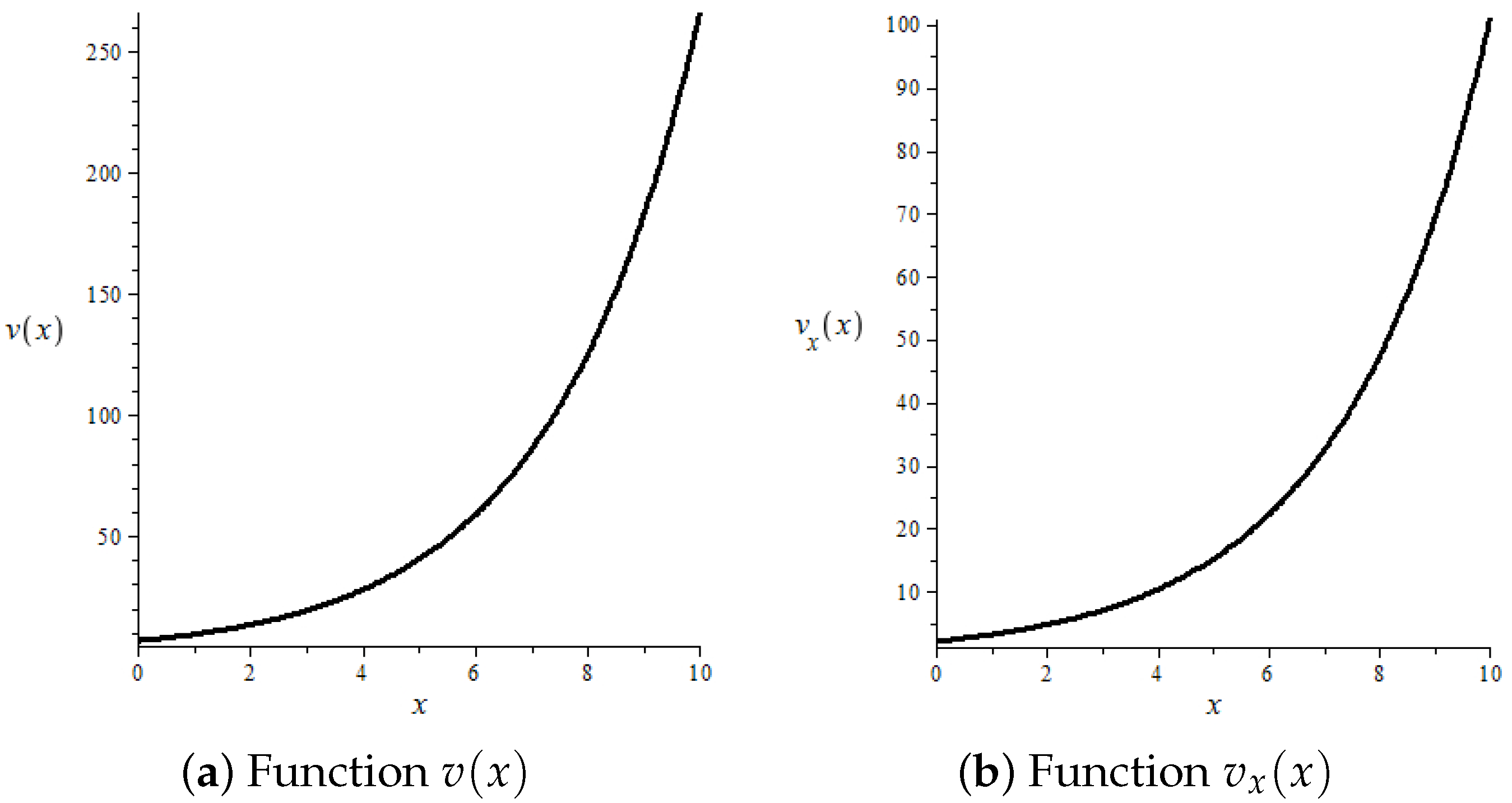
3.1. Classical Risk Process (1) and Power Utility Function
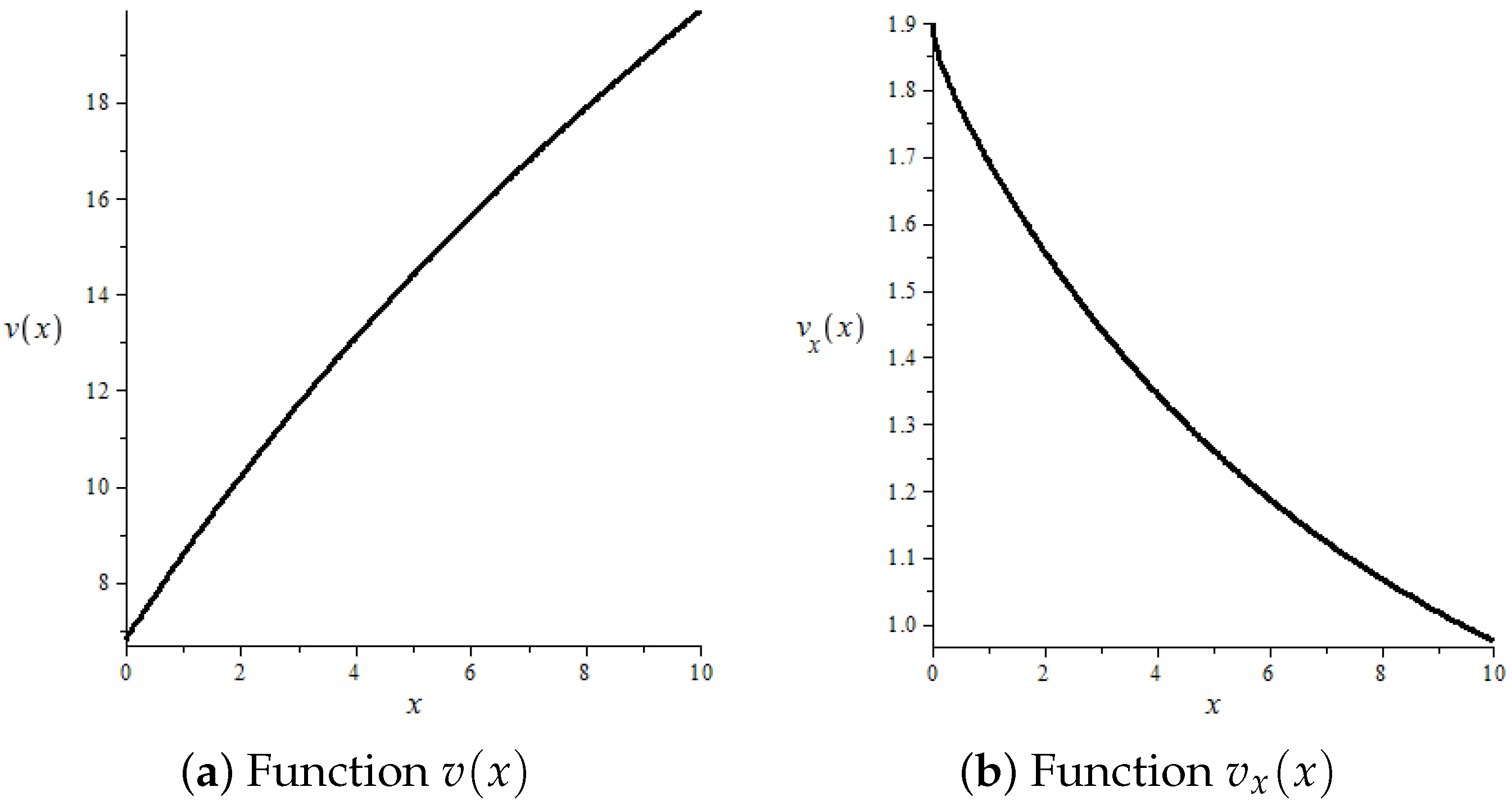
3.2. Classical Risk Process (1) and Logarithmic Utility Function
4. Numerical Analysis
- Set initial value ,
- From the equality (13) derive initial value ;
- Solve numerically the differential Equation (12) with the initial condition ;
- Calculate using ;
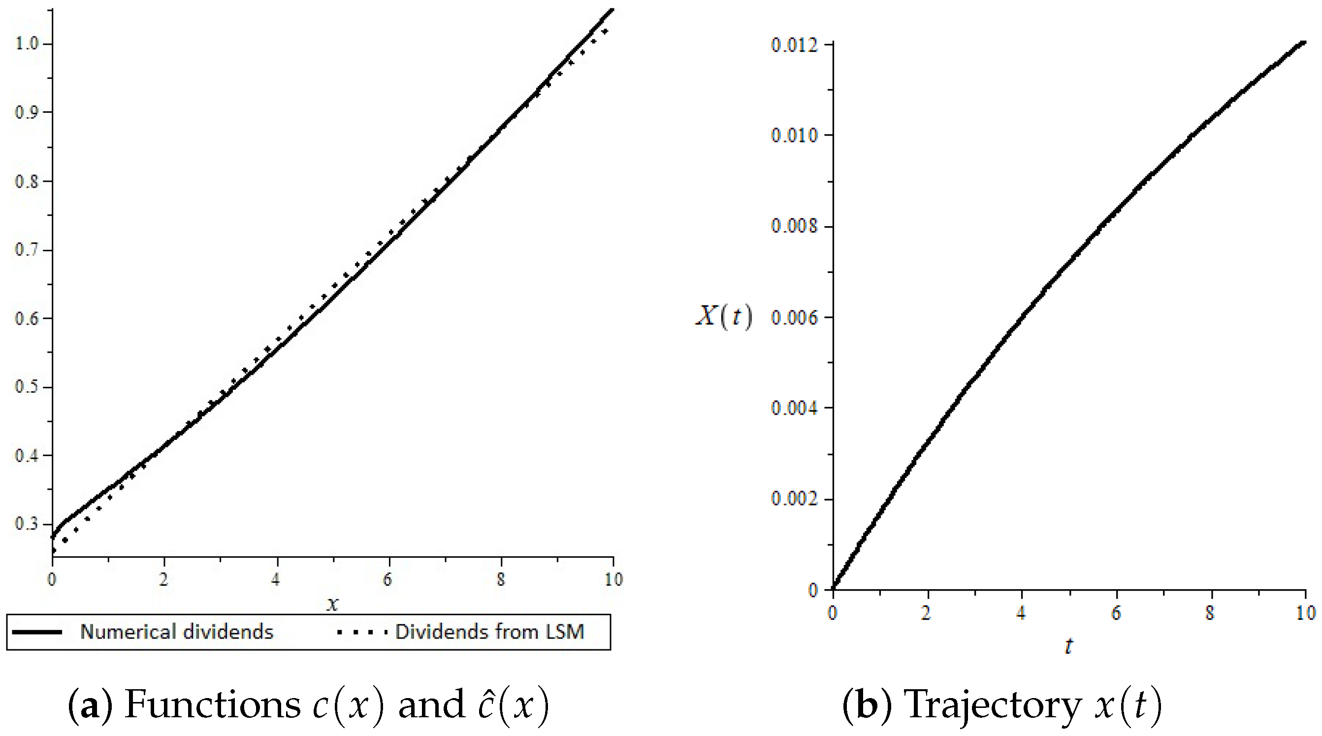
- Using the least squares method, approximate be the linear function . Because of our results from Theorem 2, we assume that is a linear function;
- Let be a trajectory of the regulated process starting from 0 until the first time claim arrival T. Hencei.e.,
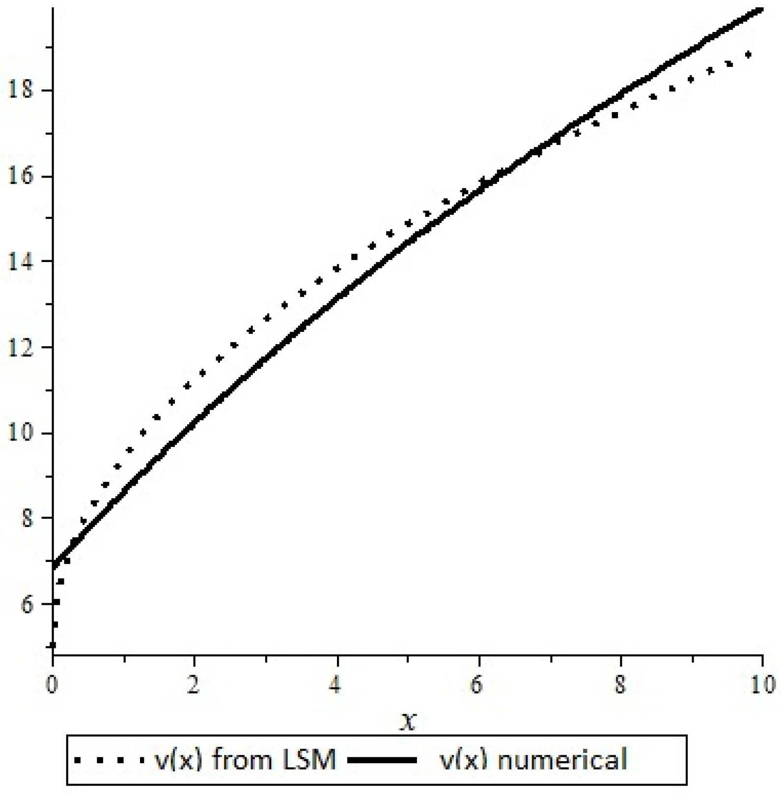
- Using the least squares method, approximate by a function of the form . Because of our results from Theorem 2, we assume that is a power function;
- Calculatewhere .
- Calculate the value ;
- Repeat until for fixed .
Author Contributions
Funding
Data Availability Statement
Conflicts of Interest
Correction Statement
Appendix A. Proof of Theorem 2
- (a)
- and ;
- (b)
- and ;
- (c)
- and .
- I.
- If , then, via the separation of variables, we have
- II.
- If , then a simple integration leads to
Appendix B. Proof of Theorem 3
- (a)
- and ;
- (b)
- and ;
- (c)
- and .
References
- Albrecher, Hansjörg, and Stefan Thonhauser. 2009. Optimality results for dividend problems in insurance. RACSAM Revista de la Real Academia de Ciencias, Serie A, Matematicas 103: 295–320. [Google Scholar] [CrossRef]
- Asmussen, Soren, and Hansjorg Albrecher. 2010. Ruin Probabilities. Singapore: World Scientific Singapore. [Google Scholar]
- Asmussen, Søren, and Michael Taksar. 1997. Controlled diffusion models for optimal dividend pay-out. Insurance: Mathematics and Economics 20: 1–15. [Google Scholar] [CrossRef]
- Avram, Florin, Zbigniew Palmowski, and Martijn R. Pistorius. 2007. On the optimal dividend problem for a spectrally negative Lévy process. Annals of Applied Probability 17: 156–80. [Google Scholar] [CrossRef]
- Avram, Florin, Zbigniew Palmowski, and Martijn R. Pistorius. 2015. On Gerber-Shiu functions and optimal dividend distribution for a Lévy risk-process in the presence of a penalty function. Annals of Applied Probability 25: 1868–935. [Google Scholar] [CrossRef]
- Azcue, Pablo, and Nora Muler. 2005. Optimal reinsurance and dividend distribution policies in the Cramér-Lundberg model. Mathematical Finance 15: 261–308. [Google Scholar] [CrossRef]
- Baran, Sebastian, and Zbigniew Palmowski. 2013. Problem optymalizacji oczekiwanej użyteczności wypłat dywidend w modelu Craméra-Lundberga. Roczniki Kolegium Analiz Ekonomicznych 31: 27–43. [Google Scholar]
- Baran, Sebastian, and Zbigniew Palmowski. 2017. Optimal utility of dividends for Cramér-Lundberg risk process. Applicationes Mathematicae 44: 247–65. [Google Scholar] [CrossRef]
- Coddington, E. A., and N. Levinson. 1987. Theory of Differential Equations. New Delhi: McGraw-Hill. [Google Scholar]
- De Finetti, B. 1957. Su un’impostazione alternativa dell teoria colletiva del rischio. Transactions of the XVth International Congress of Actuaries 2: 433–43. [Google Scholar]
- Eisenberg, Julia, and Hanspeter Schmidli. 2011. Minimising expected discounted capital injections by reinsurance in a classical risk model. Scandinavian Actuarial Journal 3: 155–76. [Google Scholar] [CrossRef]
- Eisenberg, Julia, and Zbigniew Palmowski. 2021. Optimal dividends paid in a foreign currency for a Lévy insurance risk model. North American Actuarial Journal 25: 417–37. [Google Scholar] [CrossRef]
- Gao, Hui, and Chuancun Yin. 2023. A Lévy risk model with ratcheting and barrier dividend strategies. Mathematical Foundations of Computing 6: 268–79. [Google Scholar] [CrossRef]
- Gerber, Hans U. 2012. Introduction to Mathematical Risk Theory. Cambridge: Cambridge University Press. First published in 1979. [Google Scholar]
- Gerber, Hans U., and Elias S. W. Shiu. 2004. Optimal dividends: Analysis with Brownian motion. North American Actuarial Journal 8: 1–20. [Google Scholar]
- Goldie, C., N. Bingham, and J. Teugels. 1989. Regular Variation. Cambridge: Cambridge University Press. [Google Scholar]
- Grandits, Peter, Friedrich Hubalek, Walter Schachermayer, and Mislav Žigo. 2007. Optimal expected exponential utility of dividend payments in Brownian risk model. Scandinavian Actuarial Journal 2: 73–107. [Google Scholar] [CrossRef]
- Jeanblanc-Picqué, Monique, and Albert Nikolaevich Shiryaev. 1995. Optimization of the flow of dividends. Russian Math. Surveys 50: 257–77. [Google Scholar] [CrossRef]
- Hubalek, Friedrich, and Walter Schachermayer. 2004. Optimizing expected utility of dividend payments for a Brownian risk process and a peculiar nonlinear ODE. Insurance: Mathematics and Economics 34: 193–225. [Google Scholar] [CrossRef]
- Loeffen, Ronnie L. 2008. On optimality of the barrier strategy in de Finetti’s dividend problem for spectrally negative Lévy processes. The Annals of Applied Probability 18: 1669–80. [Google Scholar] [CrossRef]
- Noba, Kei. 2021. On the optimality of double barrier strategies for Lévy processes. Stochastic Processes and their Applications 131: 73–102. [Google Scholar] [CrossRef]
- Marić, Vojislav. 1972. Asymptotic behavior of solutions of nonlinear differential equation of the first order. Journal of Mathematical Analysis and Applications 38: 187–92. [Google Scholar] [CrossRef]
- Paulsen, Jostein. 2007. Optimal dividend payments until ruin of diffusion processes when payments are subject to both fixed and proportional costs. Advances in Applied Probability 39: 669–89. [Google Scholar] [CrossRef]
- Schmidli, Hanspeter. 2008. Stochastic Control in Insurance. Berlin: Springer. [Google Scholar]
- Thonhauser, Stefan, and Hansjörg Albrecher. 2011. Optimal dividend strategies for a compound Poisson risk process under transaction costs and power utility. Stochastic Models 27: 120–40. [Google Scholar] [CrossRef]
- Zhou, Xiaowen. 2005. On a classical risk model with a constant dividend barrier. North American Actuarial Journal 9: 1–14. [Google Scholar] [CrossRef]


| x | |||
|---|---|---|---|
| 0 | 6.8021 | 1.9000 | 0.2770 |
| 1 | 8.5790 | 1.6929 | 0.3489 |
| 2 | 10.2022 | 1.5575 | 0.4122 |
| 3 | 11.7010 | 1.4431 | 0.4802 |
| 4 | 13.0940 | 1.3454 | 0.5525 |
| 5 | 14.3963 | 1.2613 | 0.6286 |
| 6 | 15.6203 | 1.1884 | 0.7081 |
| 7 | 16.7762 | 1.1247 | 0.7905 |
| 8 | 17.8723 | 1.0687 | 0.8755 |
| 9 | 18.9158 | 1.0192 | 0.9626 |
| 10 | 19.9126 | 0.9752 | 1.0515 |
| x | |||
|---|---|---|---|
| 0 | 6.8000 | 2.0000 | 0.2500 |
| 1 | 9.4022 | 3.1941 | 0.0980 |
| 2 | 13.3275 | 4.7502 | 0.0443 |
| 3 | 19.1343 | 7.0039 | 0.0204 |
| 4 | 27.6771 | 10.2878 | 0.0094 |
| 5 | 40.2103 | 15.0801 | 0.0044 |
| 6 | 58.5692 | 22.0787 | 0.0021 |
| 7 | 85.4378 | 32.3029 | 0.0010 |
| 8 | 124.7394 | 47.2425 | 0.0004 |
| 9 | 182.2094 | 69.0750 | 0.0002 |
| 10 | 266.2320 | 100.9833 | 0.0001 |
| b | ||||
|---|---|---|---|---|
| Correctness | Value | a | A | |
| t.b. | ≥1.97 | - | - | - |
| c. | 1.96 | 6.798693877 | 6.783185889 | 0.015507988 |
| c. | 1.95 | 6.798803418 | 6.784849201 | 0.013954217 |
| c. | 1.94 | 6.799092783 | 6.786580941 | 0.012511842 |
| c. | 1.93 | 6.799564767 | 6.788388955 | 0.011175812 |
| c. | 1.92 | 6.800222221 | 6.790283409 | 0.009938812 |
| c. | 1.91 | 6.801068062 | 6.792277924 | 0.008790138 |
| c. | 1.90 | 6.802105263 | 6.794392618 | 0.007712645 |
| c. | 1.89 | 6.803336861 | 6.796662198 | 0.006674663 |
| t.s. | 1.88 | - | - | - |
| t.s. | 1.881 | - | - | - |
| c. | 1.882 | 6.804464186 | 6.798652236 | 0.005811950 |
| c. | 1.8819 | 6.804479085 | 6.798679195 | 0.005799890 |
| t.s. | 1.8818 | - | - | - |
| t.s. | ⋮ | - | - | - |
| t.s. | 1.88185 | - | - | - |
| c. | 1.88186 | 6.804485051 | 6.798690050 | 0.005795001 |
| c. | 1.881859 | 6.804485199 | 6.798690322 | 0.005794877 |
| c. | 1.881858 | 6.804485348 | 6.798690594 | 0.005794754 |
| c. | 1.881857 | 6.804485498 | 6.798690867 | 0.005794631 |
| c. | 1.881856 | 6.804485647 | 6.798691139 | 0.005794508 |
| c. | 1.881855 | 6.804485795 | 6.798691412 | 0.005794383 |
| c. | 1.881854 | 6.804485945 | 6.798691685 | 0.005794260 |
| c. | 1.881853 | 6.804486095 | 6.798691958 | 0.005794137 |
| c. | 1.881852 | 6.804486243 | 6.798692231 | 0.005794012 |
| c. | 1.881851 | 6.804486392 | 6.798692504 | 0.005793888 |
| t.s. | 1.881850 | - | - | - |
| t.s. | ⋮ | - | - | - |
| t.s. | 1.8818503 | - | - | - |
| c. | 1.8818504 | 6.804486482 | 6.798692667 | 0.005793815 |
| c. | 1.88185039 | 6.804486484 | 6.798692671 | 0.005793813 |
| c. | 1.88185038 | 6.804486485 | 6.798692673 | 0.005793812 |
| c. | 1.88185037 | 6.804486486 | 6.798692675 | 0.005793811 |
| c. | 1.88185036 | 6.804486488 | 6.798692679 | 0.005793809 |
| c. | 1.88185035 | 6.804486489 | 6.798692681 | 0.005793808 |
| t.s. | 1.88185034 | - | - | - |
| t.s. | 1.881850341 | - | - | - |
| c. | 1.881850342 | 6.804486491 | 6.798692684 | 0.005793807 |
Disclaimer/Publisher’s Note: The statements, opinions and data contained in all publications are solely those of the individual author(s) and contributor(s) and not of MDPI and/or the editor(s). MDPI and/or the editor(s) disclaim responsibility for any injury to people or property resulting from any ideas, methods, instructions or products referred to in the content. |
© 2023 by the authors. Licensee MDPI, Basel, Switzerland. This article is an open access article distributed under the terms and conditions of the Creative Commons Attribution (CC BY) license (https://creativecommons.org/licenses/by/4.0/).
Share and Cite
Baran, S.; Constantinescu, C.; Palmowski, Z. Asymptotic Expected Utility of Dividend Payments in a Classical Collective Risk Process. Risks 2023, 11, 64. https://doi.org/10.3390/risks11040064
Baran S, Constantinescu C, Palmowski Z. Asymptotic Expected Utility of Dividend Payments in a Classical Collective Risk Process. Risks. 2023; 11(4):64. https://doi.org/10.3390/risks11040064
Chicago/Turabian StyleBaran, Sebastian, Corina Constantinescu, and Zbigniew Palmowski. 2023. "Asymptotic Expected Utility of Dividend Payments in a Classical Collective Risk Process" Risks 11, no. 4: 64. https://doi.org/10.3390/risks11040064