
A Model for Risk Adjustment (IFRS 17) for Surrender Risk in Life Insurance

Department of Mathematics, Stockholm University, 106 91 Stockholm, Sweden
Risks 2023, 11(3), 62; https://doi.org/10.3390/risks11030062
Submission received: 8 December 2022
/
Revised: 27 January 2023
/
Accepted: 13 March 2023
/
Published: 20 March 2023
Abstract
:We propose a model for risk adjustment, in the context of IFRS 17, for surrender risk. Surrender rates are assumed to follow a stochastic process, underpinned by data. The distribution of the present value of future individual cash flows is calculated. Using well-known techniques from the theory of convex ordering of stochastic variables, we present closed formula approximations of risk measures, such as quantiles, for the total portfolio. These formulas are easy to program and enable an insurance company to calculate its risk adjustment without time-consuming simulations.
1. Introduction
In IFRS 17, the new standard for accounting insurance contracts, a risk adjustment for non-financial risks is required. The method is not specified, but disclosing the associated confidence level is compulsory. One of the non-financial risks that can have a large impact on an insurance company is surrender risk. The purpose of this article is to calculate, and approximate, ultimo risk measures for the distribution of values of a portfolio of life insurance contracts, given the variation in surrender rates over the horizon of the portfolio, and use these risk measures to determine the required risk adjustment for this risk type.
1.1. IFRS 17
Generally speaking, the balance sheet of a company shall give a fair view of the company’s financial status at a given point in time. Similarly, the income statement shall be correct for the accounting year it reflects, in that income and cost are recognized at the relevant time. This entails a correct valuation of assets and liabilities, including future cash flows. Insurance companies differ from many others in that the income cash flows and cost cash flows often occur at times wide apart, and to a large extent are stochastic in amount and/or timing. Accounting of insurance companies hence entails particular problems.
IFRS17 (n.d.) is a new standard for the accounting of insurance contracts, published by the International Account Standards Board (IASB). It came into force on 1 January 2023, and is an attempt to solve the above-mentioned insurance-specific accounting problem and hence create better visibility for investors and improve comparability between companies. The standard is principle-based, meaning that there is some freedom for insurers to choose methods. It proposes three different models: the General Measurement Model, the Variable Fee Approach, and the Premium Allocation Approach. All require risk adjustment, but the Premium Allocation Approach is only used for short-term contracts and surrender risk will not play a large role there.
We give a brief explanation of the main principles of the standard (see also Appendix A). The first step is to put insurance contracts that have been recognized in the reporting period into portfolios with similar characteristics. Within each portfolio, each contract’s cash flows are projected over the coverage period. Typically a best estimate approach, based on expectation, is used. The cash flows are then adjusted for the time value of money, i.e., discounted, and for other uncertainties due to financial risks. For instance, the discount rate shall incorporate illiquidity adjustment. The result after this step is called the Present Value of Future Cash Flows (PVFCF). The next step is a requirement of a risk adjustment for non-financial risks for the portfolio of contracts. In life insurance, biometric risks are typical examples, and so is surrender risk. The purpose of the risk adjustment is to “reflect the compensation that the entity requires for bearing the uncertainty about the amount and timing of the cash flows that arises from non-financial risk” (IFRS17 n.d., § 37). There is no prescription of the model for risk adjustment. It is up to the company to choose, but there are five criteria that the model must fulfill, and both the model and the confidence level must be disclosed (IFRS17 n.d., § B91). The sum of the PVFCF and the risk adjustment is called the fulfillment cash flow. Finally, if a contract gives rise to a gain on day 1, this amount is called the contractual service margin and must be included in the liabilities and released into the income statement over the course of the contract. On the other hand, onerous contracts (giving rise to a loss on day 1) must be fully recognized in the income statement immediately. We refer to Palmborg et al. (2021) for an overview of IFRS 17 and its challenges, including an illuminating mathematical description.
The risk adjustment for non-financial risk is further discussed in IFRS17 (n.d., §§ B86–B92), but no explicit method is given. There are basically two approaches to risk adjustment: either a confidence level-based method is used (sometimes this is called the percentile method or, slightly misleading, Value at Risk), or another method is used where the confidence level is not explicit. In the latter case, the confidence level must then be estimated.
In the percentile method, a chosen quantile of the distribution of cash flows, under uncertainty due to non-financial risks, is calculated. A weakness of the method is that the economic motivation for choosing one or the other quantile is unclear. Nevertheless, it is one of the approaches in use, due to its simplicity, and it is the route we will take here.
The risk adjustment bears some resemblance to the risk margin in Solvency II; however, there are important differences. The confidence level is given in Solvency II, and the risk margin is calculated by a prescribed cost of capital method, where even the cost of capital rate is explicitly given. However, there are also more fundamental differences. Solvency II takes the perspective of another player on the market who is interested in taking over the business, and the risk margin is compensation for the non-financial risks in this takeover. On the other hand, in IFRS 17, it is the company’s view of risk that shall be guiding the model choice, the confidence level included. Further, the Solvency II risk margin is based on a one-year perspective, whereas the IFRS 17 takes the more classical actuarial view of all cash flows during the lifetime of the contract, cf. England et al. (2019). Nevertheless, the cost of capital method is one of the methods in use. In principle, this is economically sound, but the choice of the rate is not easy, and the requirement to disclose the confidence level is a further challenge of this method.
1.2. Our Objective and Setup
Since the principles of IFRS 17 were first proposed and published, the method for risk adjustment has been widely discussed within the insurance industry, and in particular the actuarial community. There has certainly been a number of white papers (e.g., Boumezoud et al. 2020 and IAA 2018), seminars and alike where risk adjustment has been discussed, but to the best of our knowledge, very little research has been published on the topic. The risk adjustment is, however, treated in England et al. (2019). Although devoted to non-life insurance, the article contains a general and interesting discussion on the nature of the risk adjustment, and, in particular, the differences between it and the Solvency II Risk margin.
Many companies have been (and still are) struggling to find methods for risk adjustment that are based on sound models, that fulfill the five criteria, that are easy and quick to calculate, and where the confidence level can be determined. It is our impression that no method has yet become the best practice. A survey in 2018 (Smith et al. 2019) showed that 53% of the companies in the sample were aiming for a cost of capital method, whereas 33% planned to use a Value at Risk method. The present work has grown out of practical needs, and our objective is to present a method for surrender risk, and thus to start filling the gap in the literature.
The outset is a portfolio of life insurance contracts with similar risk characteristics. The customers pay the insurance company’s annual premiums and will receive a predefined payment at death if they are still in the portfolio. We assume no new customers entering the portfolio, but that surrenders happen. By value we mean the above-mentioned PVFCF1 from this portfolio given the stochastics for the surrender rate (but keeping other parameters constant) over the horizon of the portfolio. The focus is on ultimo risk measures for the value, where “ultimo” is added to distinguish these risk measures from the one-year method in the Solvency II standard formula, where the risk factor is stochastic the first year but then stays constant for the remaining years. The measures we will treat are (i) a suitable quantile of the distribution of the value, and (ii) the partial expectation up to such a quantile.
We present two alternative stochastic processes for surrender rates; they are chosen for their mathematical tractability and underpinned by data from a life insurance company. We will see that, depending on the product and the surrender experience, one of the models is better suited than the other for risk adjustment modeling.
Applying techniques from the theory of convex ordering of stochastic variables, we then find closed formulas approximating the two ultimo risk measures for each of the two model specifications. There is a rich literature on convex bounds for approximating sums of stochastic variables with various financial applications (cf. Section 3). We are not contributing to this domain of research, but rather developing existing tools for usage in another area of application.
One advantage of the presented method is to avoid simulations that could be time-consuming for large portfolios, and also subject to random errors leading to the fluctuation in the risk adjustment. We also show that the method fulfills the criteria in IFRS 17.
1.3. Risk Measures
For a random variable, we define the two risk measures quantile at confidence level p as
where is the cumulative distribution function of X, and the partial expectation at confidence level p as the average of the quantiles
(We avoid the terms “Value at Risk” and “Conditional Value at Risk” as these normally refer to a loss variable, while we consider a value variable.)
We will use the lognormal distribution extensively, so here we collect some results about it. Let X be a random variable such that is normally distributed with mean and variance . Then we say that X is lognormal with parameters . Let denote the cumulative distribution function of the standard normal distribution, and the quantile at confidence level p of this distribution. Then we have
1.4. Outline of the Article
Stochastic modeling of surrender rates is discussed in Section 2, where the two models are introduced and the risk measure for a cash flow at a future point in time is calculated. We also motivate the models with empirical data.
Section 3 introduces well-known concepts of convex ordering and comonotonicity with application to risk measures and in particular sums of lognormal stochastic variables.
In Section 4, we apply the machinery presented in Section 3 to derive approximations of the risk measures of the total PVFCF. All necessary parameters are calculated and presented in terms of the (discounted) cash flows. We also present a stylized example that shows the accuracy of the approximations.
Section 5 discusses the practical application of the method; the estimation of parameters is discussed, as well as the explicit choice of risk adjustment. The model is compared to regulatory criteria for risk adjustment.
Section 6 is conclusions.
2. Stochastic Modelling of Surrender Rates
2.1. Introduction
Surrender rates are contingent on customer behavior, and thus difficult to model. They may depend on diverse endogenous and exogenous factors such as contract design (e.g., fees for surrenders or not), macroeconomics (e.g., interest rates, unemployment), portfolio properties (e.g., distribution of age of contracts), change in regulations, or company-related events (such as incidents leading to loss of reputation). There is a rich literature on models of surrender rates in life insurance in the context of such explanatory factors. For a survey of this research up to 2013, we recommend Eling and Kochanski (2013) and references therein; it also contains a classification of different types of models. See also Barsotti et al. (n.d.) and Milhaud and Dutang (2018).
As our current interest is to construct a reliable risk adjustment, we take a more humble position and do not forecast customer behavior based on explanatory factors. Our focus is on the portfolio as a whole and observed surrender rates (in proportion to the number of in-force contracts) are our data. Typically the company has a best estimate of the surrender rate, revised yearly. Using this estimate as a start value, we use historical volatility to forecast the future volatility of surrender rates. These fluctuations may be seen as the aggregate of the environmental factors mentioned above.2 We will look at two alternative models, one where the rates fluctuate around its best estimate, and one where the rates have a “stickiness” property, but without drift; we propose a Markov process that is a martingale.
Let us assume that the company has calculated the future net cash flows for each year , given a surrender rate of zero. Each cash flow is the net of the premium income minus insurance outpayments and expenses. These components are calculated given actuarial assumptions, in particular mortality. If desired, they can also be seen as discounted. The PVFCF from the portfolio is
We now introduce surrenders into the picture. Let c be the best estimate at time 0 for the surrender rate. For technical reasons we will model the “remain rate” instead of the surrender rate; let this be at time 0. Now assume that the remain rate follows some process , . Each year t, a proportion of contracts equal to remain. Obviously, this means that the net cash flows will be lower than those with no surrenders (given that they are positive). We make the simplifying assumption of homogeneity: all contracts have the same probability to remain at time t, in particular, subportfolios (e.g., for different products) have the same expected remain rate, and the remain rate does not depend on the contract’s time to maturity. Then, the net cash flow will be proportional to the state model, leading to a modified cash flow at time t:
The total PVFCF becomes
Typically we will have a cash flow and we want to make a risk adjustment for situations when the cash flow becomes lower than expected.
2.2. The Poisson Process
A standard model of surrenders is the Poisson process. This means that the number of surrenders L in a time interval of length 1 is , where is the intensity. Allowing for stochastic intensity in such a process leads to a Cox process, cf. Grandell (1991). More precisely, let be a stochastic process, independent of the individual surrenders. Conditional on the intensity , let the number of surrenders in the time interval be . Defining , where N is portfolio size at the beginning of the time interval, we see that the conditional expectation of R, given , is and its variance is . For large portfolios, the variance is close to zero, and the conditional distribution of R is close to a Dirac distribution at .
2.3. Discrete Time
Motivated by this, we model the remain rates directly, i.e., ignoring arrivals of individual surrenders. We will look at the “lognormal model”, where rates are defined as
and the “sticky model” where the remain rate is calculated by a multiplicative shock on the previous remain rate:
where are standard normal and independent variables and is a constant parameter. According to (3), for the lognormal model, and for the sticky model, i.e., is a martingale. Still, both models could lead to remain rates larger than 1. We will basically ignore this artifact of the model; it will be discussed in Section 4.2.
As we will see, both models are mathematically pleasant to work with. The relevant question of whether they are realistic will be discussed in Section 2.6.
2.3.1. The Lognormal Model
We have
where .
As the are independent standard normal, each is a normally distributed variable with mean 0, and the covariance matrix C of , is given by
In particular, the variance of equals t. Hence, using (3), the quantile at confidence level p of is
The partial expectation is
2.3.2. The Sticky Model
Using (8) recursively, we get
Define and recall that . Then
Again, as the are independent standard normal, each is a normally distributed variable with mean 0, and the covariance matrix C of , is calculated as follows. Assuming , we obtain
In particular, the variance of equals . Hence, using (3), the quantile at confidence level p of is
The partial expectation is
2.4. Continuous Time
Another approach is to work in continuous time. We will do this for the sticky model only. Let be the share of remaining contracts at time t, . We get in a small time interval :
Define . Then , i.e., . Integrating this equation, we obtain
Now, let us assume that follows a Geometric Brownian motion , . It is well known that the solution can be expressed as . Thus
Call the last integral . It is a time integral of a Brownian motion which can be evaluated using Itô calculus; it can be shown that is a Gaussian process, i.e., for any finite collection of times , the corresponding random variables are multivariate normal. In addition, , , and for . Hence
where is standard normal. Changing back to N, we get
Hence,
whose p-quantile is
This expression of the quantile and the one derived in discrete time are very close. The partial expectation is
2.5. Term Structure of Surrender Rates
The assumption of a single best estimate for the surrender rate (and hence the remain rate) is in some cases too restrictive. Rather one has a term structure of expected remain rates in year t, due to known properties of the portfolio. For instance, as time passes, the customers’ average age increases which may influence the remain rate. Then the sticky model can be generalized as follows.3 Assume that the stochastic remain rate in year t is
This means that the remain rate is influenced by the cumulative shocks up to the year in question. The cash flow in year t then becomes
In the lognormal case, the calculations and result are similar, only simpler. The conclusion is that the term structure does not essentially complicate the model; it changes only the deterministic factor in each . To simplify the notation, in the remaining part of the paper we will work with the case of a constant best estimate r.
2.6. Realism of the Models
The two models obviously have very different properties, and one can be favored over the other because of some known properties of the portfolio/product. However, we recommend choosing the model only after testing both of them on the historical data.
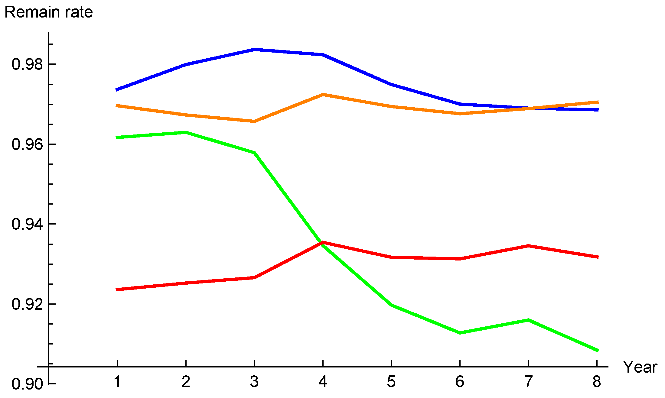
We have tested the two model assumptions on four portfolios from a life insurance company. These are all term-life insurance, but they differ in terms of the composition of clients, for instance, two of the portfolios have been closed for some time so their clients have higher average ages. The time series covers eight years and the corresponding remain rates are shown in the graph, Figure 1.4
For each of the four portfolios, we first logarithmize the time series of remain rates. The lognormal model is a good fit if the logarithmized time series itself is close to normal, cf. (7), and the sticky model is a good fit if the consecutive differences of the logarithmized time series are close to normal, cf. (8). To test this, we perform the Shapiro–Wilk test on these two cases. The Shapiro–Wilk test fails, i.e., the null hypothesis of normality is rejected, when the p-value is below a given threshold, e.g., 0.10. Comparing the p-values for the two models indicates which of them is more suitable.5
The results are as follows (p-values for the lognormal model to the left and for the sticky model to the right).
We observe that the normality is rejected only for the green portfolio and the lognormal model, but also that the sticky model is far more realistic for all of the products except the orange one. The choice between the two models can be based on an analysis of historical data such as this test, or a Q-Q plot of the quantity against the normal distribution, and then of , to examine which gives a better fit.
Both the proposed models have zero drift. If we have good reasons to believe that a certain trend is expected going forward, this can be incorporated by using the term structure in the previous subsection. Historical data is used to estimate the volatility, see Section 5.1, but a historical trend will not automatically influence the rates going forward. This is a virtue of the model
We remark that the two proposed models are special cases of the AR(1) model , and estimating the parameters in this model will give an even closer fit to data. However, we do not recommend this choice, as there is a risk of overfitting; in addition, this model will generally have a drift, and it is not obvious how to combine it with the expected term structure.
3. Convex Ordering of Random Variables and Its Applications
To date, we have calculated the distribution of the cash flow for an individual year in the future. Before continuing to the total portfolio, we will now make a diversion and present some known results about convex ordering of random variables and their application to approximations of risk measures. There is a rich and recent literature on the convex ordering of stochastic variables, and upper and lower convex bounds of sums of lognormal variables, for different financial applications. In this direction, we mention Deelstra et al. (2008); Linders and Stassen (2016) and Hanbali and Linders (2019) (application to basket options), as well as Chaoubi et al. (2020) and Hanbali et al. (2022) (counter-monotonic risks).
For a good introduction to the topic, we refer to Dhaene et al. (2006), on which a large part of the material in this section is built.
3.1. Definition of Convex Ordering
There are different ways to introduce partial orderings between random variables. The most obvious is to compare their distribution functions. Let X and Y be two random variables.
Definition 1.
X is said to precede Y in the stochastic dominance sense, notation , if
for all x.
Obviously, the stochastic dominance ordering preserves quantiles, i.e., for all , so the respective quantiles of X and Y are ordered. However, for our purposes, a weaker sense of ordering is often natural.
Definition 2.
X is said to precede Y in the convex order sense, notation , if
for all convex functions v.
The essence of the convex ordering is that the dominating variable Y is riskier, its tails are “larger”. Note that, as and are convex, a necessary condition for is that . As a simple example, let X be the constant (no other constant would work). Then, by Jensen’s inequality, we get for any convex function v,
so .
Further, it can be shown that the property is tail-symmetric, .
Theorem 1.
if and only if and
for all d, where .
The essence of the theorem is that rather than testing the inequality of the definition for all convex functions, it suffices to test it for all functions , which obviously are convex. The expectations in the theorem are called the stop-loss premiums for the given random variable, and the stop-loss level d. This theorem shows the usefulness of convex ordering for actuarial purposes.
3.2. Comonotonicity
A situation that often occurs in practice is a random vector where the marginal distributions are known, but the joint distribution is not. One might ask for “the extreme case”, i.e., some dependence structure that keeps the marginals but dominates all other possible joint distributions in some sense.
Let U be a (0, 1) uniformly distributed random variable, i.e.,
In the sequel, the letter U will always denote such a variable.
The so-called probability integral transform states that for any continuous random variable X, the random variable has a uniform distribution on , i.e., where the symbol means equal in distribution.
Definition 3.
The random vector is said to be co-monotonous if there exist non-decreasing functions defined on such that
where U is a uniformly distributed variable on .
The random vector Y is in a sense one-dimensional; all of its components move with U. If is strictly increasing, the marginal distribution of is , if . So is the quantile function of .
The fact that all the components of a co-monotonous random vector move with U makes it easy to calculate the risk measures:
Proposition 1.
Quantiles and partial expectations are additive for comonotonic risks , i.e., for all we have
and
3.3. Convex Bounds for Sums of Random Variables
We now state a theorem that will prove useful for approximations in the problem under study.
Theorem 2.
Let be any random vector, U as before, and Λ any random variable. Then
For the proof of the right bound6, see Kaas et al. (2000). It is instructive to look at the proof of the left bound. Let v be any convex function. We need to show that
Using the law of total expectation and Jensen’s inequality for conditional expectation, we obtain
and the statement follows by the linearity of the last conditional expectation.
The left bound is very useful, in particular when resembles in some way. In fact, if and S are independent, then the left bound reduces to the previously mentioned relation . On the other hand, if , we also get this. These examples show that a non-trivial bound requires a clever choice of .
3.4. Applications to Risk Measures
We will now investigate how quantiles and partial expectations behave in relation to convex ordering. The following simple example shows that quantiles are not preserved by convex ordering. Let X be uniform and Y be uniform . Then and , so for and for . Still, it is obvious that . In fact, the example is more typical than one might think; Ohlin’s lemma (Ohlin 1969) says that if two stochastic variables X and Y have the same expectation and their distribution functions cross exactly once, i.e., for and for , then . Ohlin’s lemma has been extended in different directions (Hesselager 1993).
The good news is that partial expectations are preserved under convex ordering.
Theorem 3.
If , then
For a proof, see Denuit et al. (2005, pp. 152–54).
3.5. Application to Sums of Lognormal Variables
We will apply approximation methods induced by convex ordering discussed above. The inspiration comes from Kaas et al. (2000, pp. 160–63), where similar cases are treated in detail. For the convenience of the reader, we will present some material from that article, with slightly changed notation.
Let
where has a multivariate normal distribution. Define
and
for some coefficients . Then has a normal distribution. Conditionally on , has a normal distribution, and we may use well-known formulas for conditional multivariate normal distributions to obtain
and
where is the correlation between and , is the standard deviation of , and is the standard deviation of . Hence, conditional on , is lognormal with expectation
In this expression, all symbols are constant, except which is a standard normal variable that can be denoted for U uniform, by the probability integral transform. Hence, defining
we end up with
and we may apply the left bound in (36) to conclude that . Note that the concluded inequality holds regardless of the choice of coefficients ; in the application, we will choose these to achieve a close bound. If, in addition, all and all , is a sum of co-monotonous variables. This means that all quantiles of are additive, and so are partial expectations.
Further, define (for non-negative )
Then, using the right bound in (36), we see that , and it is also a sum of co-monotonous lognormal variables, so
Applying this to the cash flow modeling in Section 2.1, we see that each term in (48) is the quantile of the cash flow at time t; we may call this expression the “sum of quantiles” whereas the correct risk measure is the “quantile of sum”.
4. PVFCF for the Total Portfolio
Working in discrete time, we now want to study the total PVFCF .
Using (9), we get:
in the lognormal case, and using (14) we get
in the sticky case, where , , and are independent standard normal.
In order to simplify the notation, define in the lognormal case, and in the sticky case, so that
and
respectively.
We are left with a sum of correlated lognormal distributions7.
4.1. Approximations by Convex Ordering
We will now apply the approximation from Section 3.5. Recall that this applies to expressions of the type
where has a multivariate normal distribution.
In the lognormal model, we may apply this with , and in the sticky model with . We define
and
where the coefficients will be chosen later.
4.1.1. The Lognormal Model
Define
Then
We will calculate all the constants that appear in the expression (45) for . Firstly,
and
Further,
and hence
For the choice of coefficients , we propose using
a choice that is motivated by linearization of S (cf. Kaas et al. 2000, p. 164). If all are non-negative, then the same holds for all , and hence for all .
Plugging all these parameters into Equations (45) and (47), we obtain
and
Given that all are non-negative, these expressions are sums of co-monotonous stochastic variables.
4.1.2. The Sticky Model
Define
The calculations in this case are similar, only slightly more complicated. Firstly,
and
Further,
and hence
For the choice of coefficients , we propose using
as in the previous case. If all are non-negative, then the same holds for all , and hence for all .
Again, plugging all these parameters into Equations (45) and (47), we obtain
and
Given that all are non-negative, these expressions are sums of co-monotonous stochastic variables.
4.2. Numerical Example
We will now apply the machinery to a portfolio of contracts. For simplification, we let for all t, i.e., except for surrenders there are no changes in the portfolio over time. Let , i.e., the best estimate of the surrender rate at is 4%. The horizon will be years. With no randomness, the cash flows will decrease exponentially as , so at it is down to 0.086.
4.2.1. The Lognormal Model
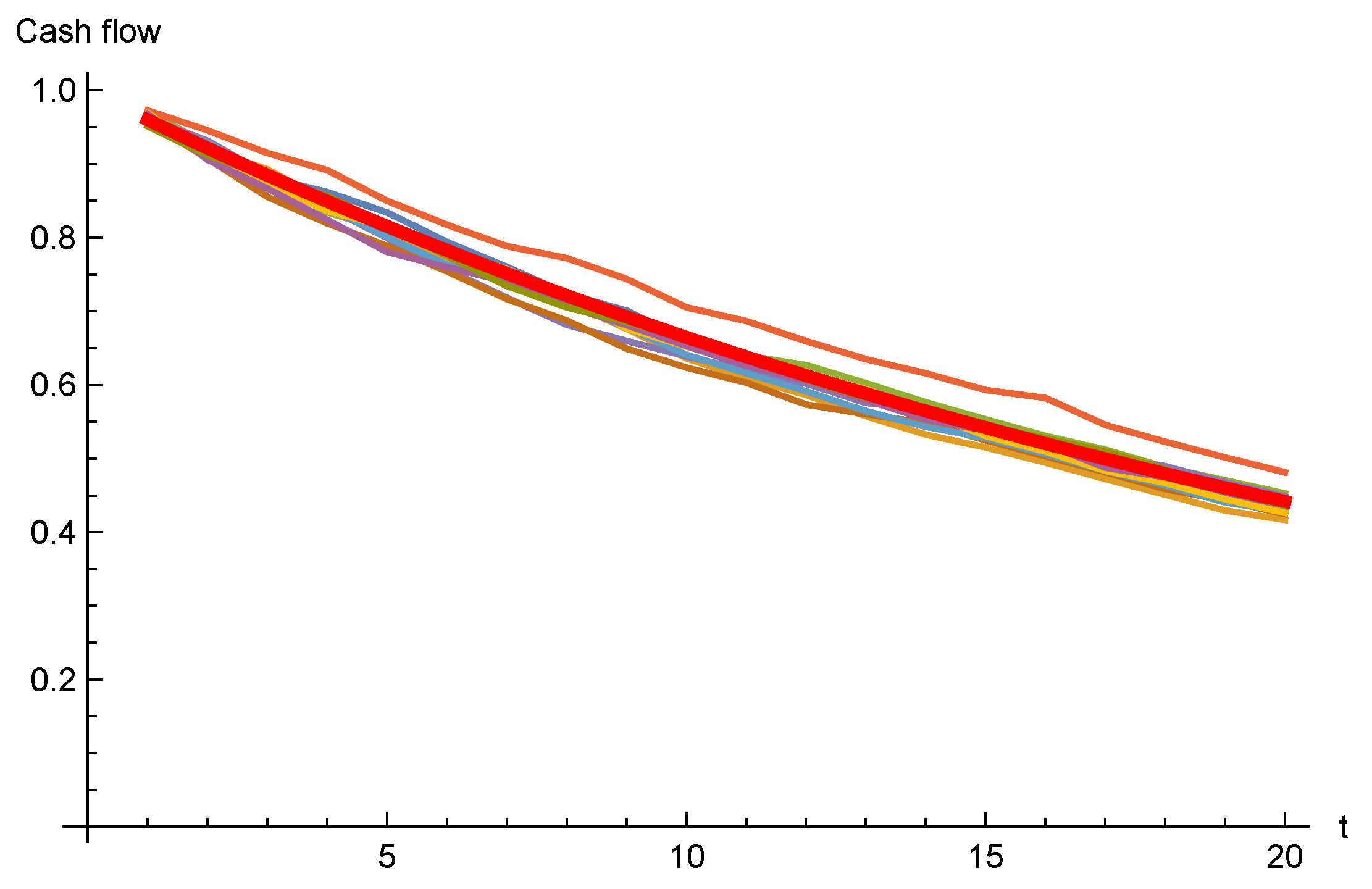
Assuming , we may simulate the cash flows; Figure 2 shows simulated paths for the first 20 years.
As the cash flows for individual years are independent in this model, the law of large numbers applies, and the simulated cash flow paths are very close to the deterministic path. The risk adjustment will be very small if we use this model. In addition, as all quantiles are so close to the mean, the approximations are of limited use. Hence, for brevity, we will continue the example for the sticky model only.
4.2.2. The Sticky Model
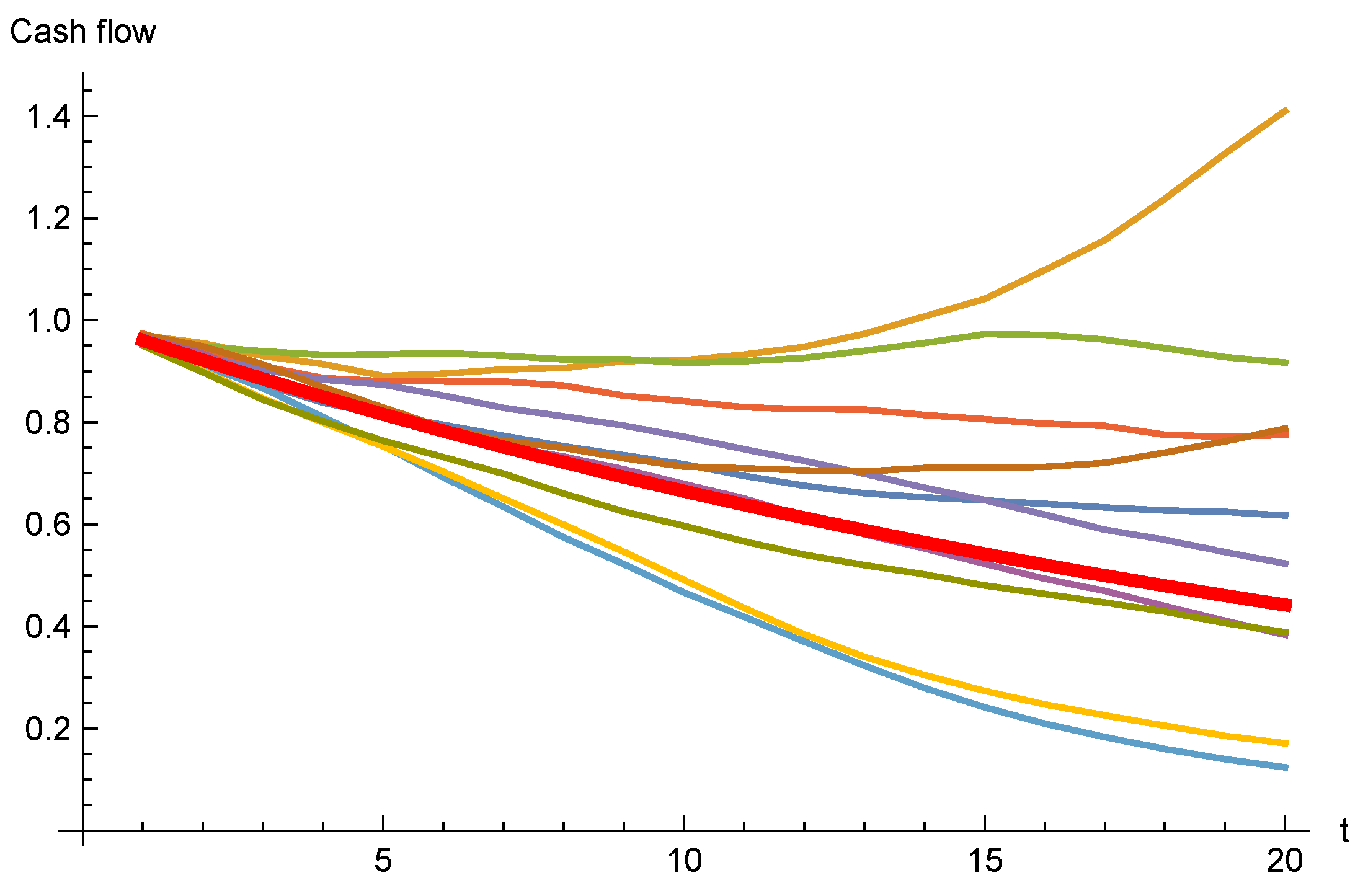
Assuming the same volatility as in the previous case , we may simulate the cash flows; Figure 3 shows simulated paths.
As expected, the variation in the cash flows is much higher for the sticky model.
We see that some paths bend upwards. This is a result of the previously mentioned fact that the model may produce remain rates . Once in that region, the remain rate may also stay there for a while. In practice, this has little influence on the end result; we are considering lower quantiles of cash flows which typically correspond to paths where the remain rate is lower than the starting point.
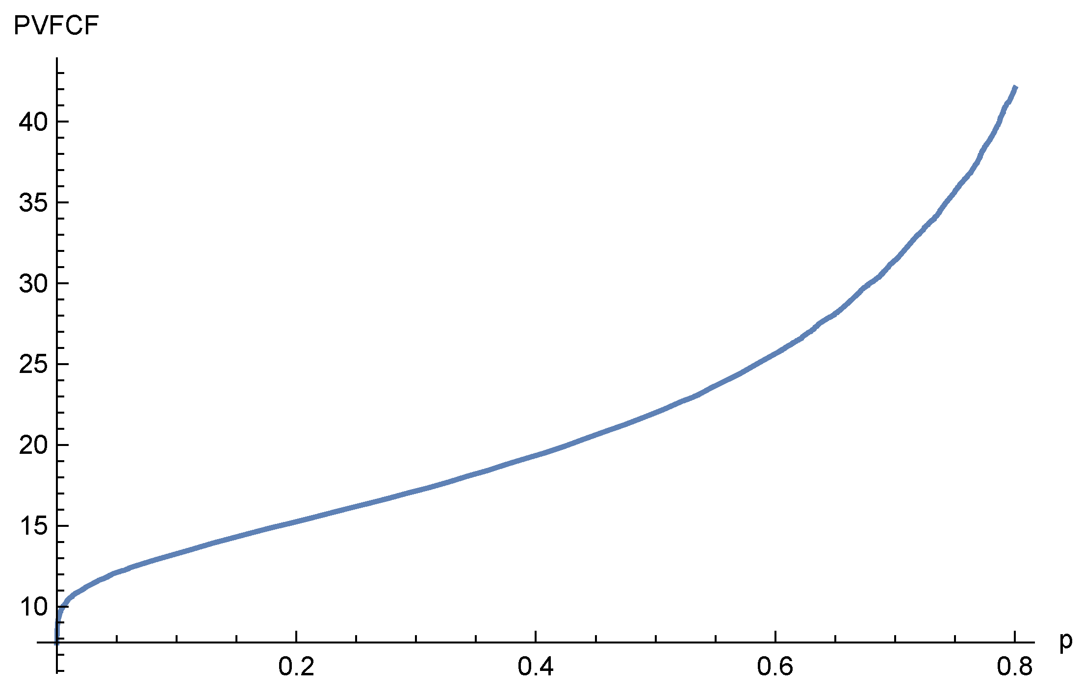
A Monte Carlo simulation will be used to construct the true distribution of the cash flows and to calculate the risk measures. Drawing 10,000 paths for cash flows, we may aggregate them in different ways. Firstly, we can add up the cash flows for each path, and look at the distribution of these sums, i.e., the random variable S. The quantile function of the total looks like this (Figure 4).
As seen, the 20% quantile of the total is 15.2. The partial expectation is easily calculated as the mean of the 20% worst outcomes; it is 13.0.
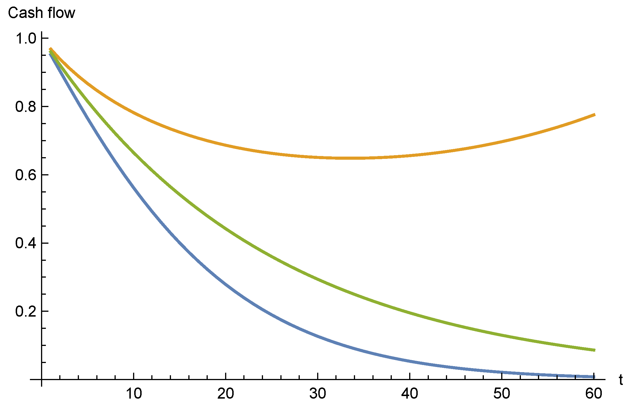
Secondly, we may also calculate the distribution for each point in time, this can be done exactly, without simulation. The green line shows the cash flows without randomness, and the other two lines show the 20% and 80% quantile, respectively, (Figure 5).
Adding up the quantiles, using the comonotonicity, we get the 20% quantile for , which is 14.7. Comparing with the quantile of S, we see that it is a conservative approximation, which is expected as .
Finally, we want to use the variable for approximation. The quantile of is then calculated by (45) and the parameters from Section 4.1.2. It is 15.2, i.e., very close but slightly lower than the simulated value; we remind the reader that the convex ordering might not preserve quantiles.
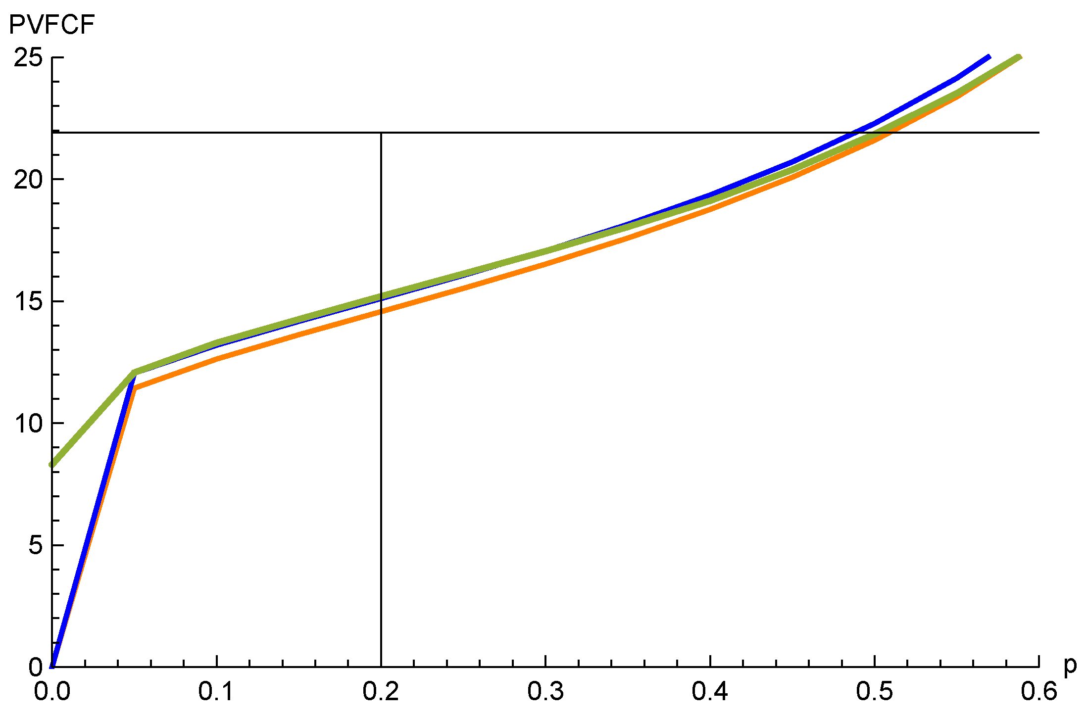
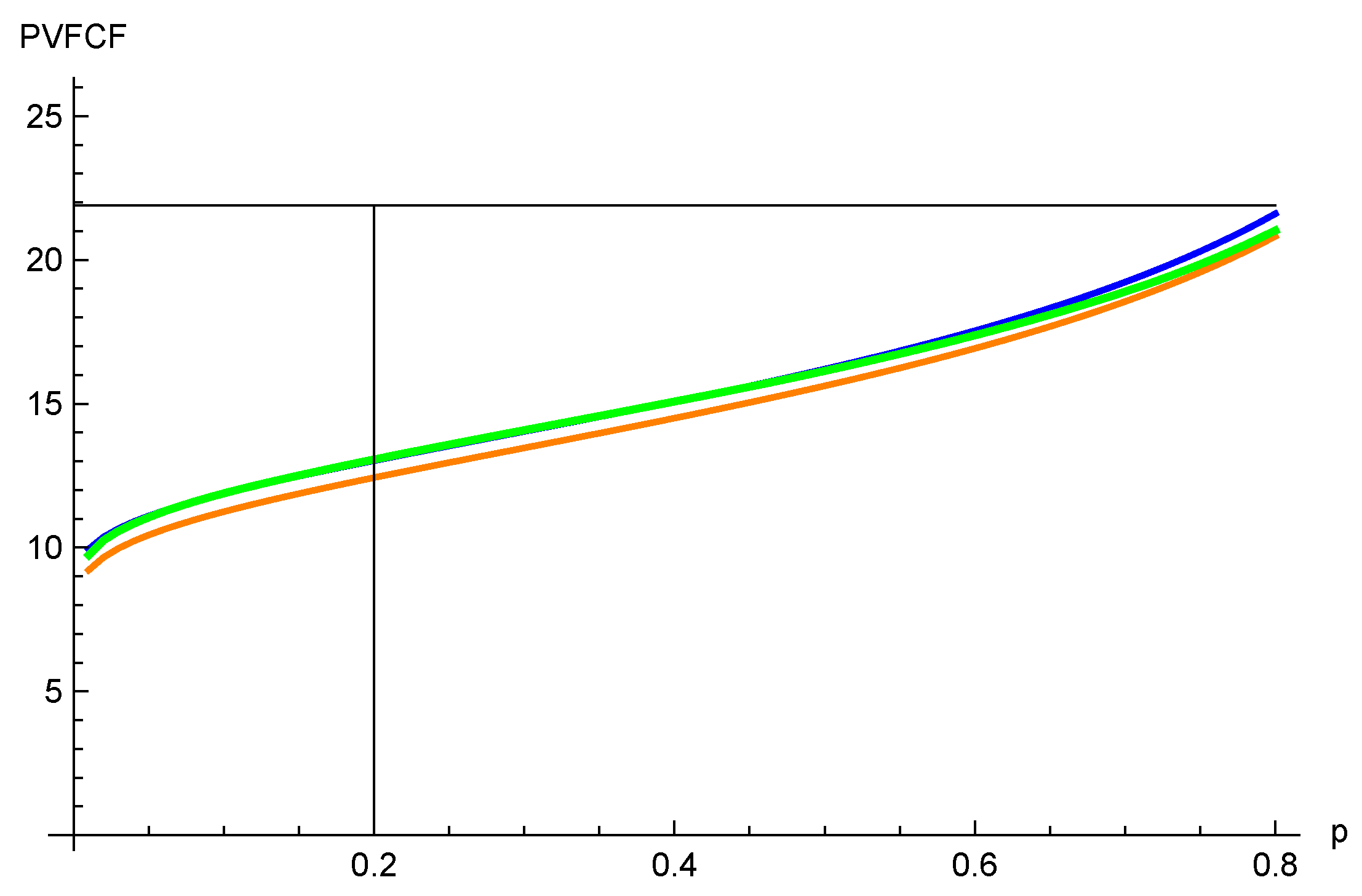
A plot of the quantile of S, , and for p between and is shown in Figure 6, and of partial expectation in Figure 7.
In both these graphs, the orange line is , the blue line is , and the thicker green line is S. The partial expectation graphs are nicely ordered, as expected. This is not the case for the quantile graphs, but it is striking how good an approximation is for the quantiles we are interested in (below 0.5). Even gives a reasonable, although conservative, approximation.
5. Implementation for Risk Adjustment
5.1. Parametrization
The model requires forward-looking estimation of the parameters and r (or a term structure ). For the latter, typically expert judgment is used based on (recent) experience and known properties of the portfolio.
The volatility is obviously very important for the size of the risk adjustment. To estimate it, the standard procedure is to use a historical time series of surrender rates , transform it into remain rates , and then calculate the sample standard deviation of the time series for the lognormal model, or for the sticky model.
For the sticky model, this is not fully correct, as the sample standard deviation measures deviations from the sample mean, whereas our model specification has the mean . This is normally close to zero, and if the historical time series has a trend, its sample mean can deviate from zero. A more correct estimate can be found by maximum likelihood estimation. The log-likelihood function is
where n is the number of observations. Differentiation with respect to gives
which leads to the estimate
For the portfolios in Section 2.6, the ML estimation gives a 25% higher volatility than the classical estimation for the green portfolio (which has a clear trend), whereas, for the other portfolios, it gives slightly lower volatility (up to 8% lower).
For the lognormal model, this problem does not occur, as the model specification has the mean , and here r is a free variable, so the maximum likelihood estimate is equal to the usual sample standard deviation.
In practice, there might be some obstacles to this estimation procedure. For instance, the history could have spikes due to idiosyncratic events that are deemed not to be repeated going forward and need to be adjusted for.
5.2. Risk Adjustment
Let us define the absolute risk adjustment , and the relative risk adjustment for surrender risk as , where X is the stochastic variable of PVFCF, given the volatility , and Y is the deterministic PVFCF when the remain rate is constant over the horizon T. Recall that IFRS 17 requires that the chosen confidence level of the risk adjustment is disclosed, and with this choice of method, it is given by definition.
Another choice is to define the risk adjustments using partial expectations instead of quantiles in the risk adjustment formulas. This has certain advantages, as discussed above, but then the question arises about which confidence level this corresponds to. Obviously, , so it may be argued that the confidence level using the PE method for risk adjustment is different from p.
5.3. Fulfillment of Criteria in IFRS17
In IFRS17 (n.d., § B91), it is stated:
“IFRS 17 does not specify the estimation technique(s) used to determine the risk adjustment for non-financial risk. However, to reflect the compensation the entity would require for bearing the non-financial risk, the risk adjustment for non-financial risk shall have the following characteristics:
- (a)
- risks with low frequency and high severity will result in higher risk adjustments for non-financial risk than risks with high frequency and low severity;
- (b)
- for similar risks, contracts with a longer duration will result in higher risk adjustments for non-financial risk than contracts with a shorter duration;
- (c)
- risks with a wider probability distribution will result in higher risk adjustments for non-financial risk than risks with a narrower distribution;
- (d)
- the less that is known about the current estimate and its trend, the higher will be the risk adjustment for non-financial risk; and
- (e)
- to the extent that emerging experience reduces uncertainty about the amount and timing of cash flows, risk adjustments for non-financial risk will decrease and vice versa.”
We now briefly discuss our proposed method’s fulfillment of these criteria.
(a) Surrenders are by nature high frequency and low severity. Nevertheless, a mass lapse event could be seen as low frequency and high severity. To model such events, the proposed model needs to be generalized to cater for jumps in , but such a model would be very hard to parametrize.
(b) Using the RRA defined in the previous section, in combination with (16):
we obtain (note that )
It is easy to verify that the risk adjustment increases with a longer horizon t.
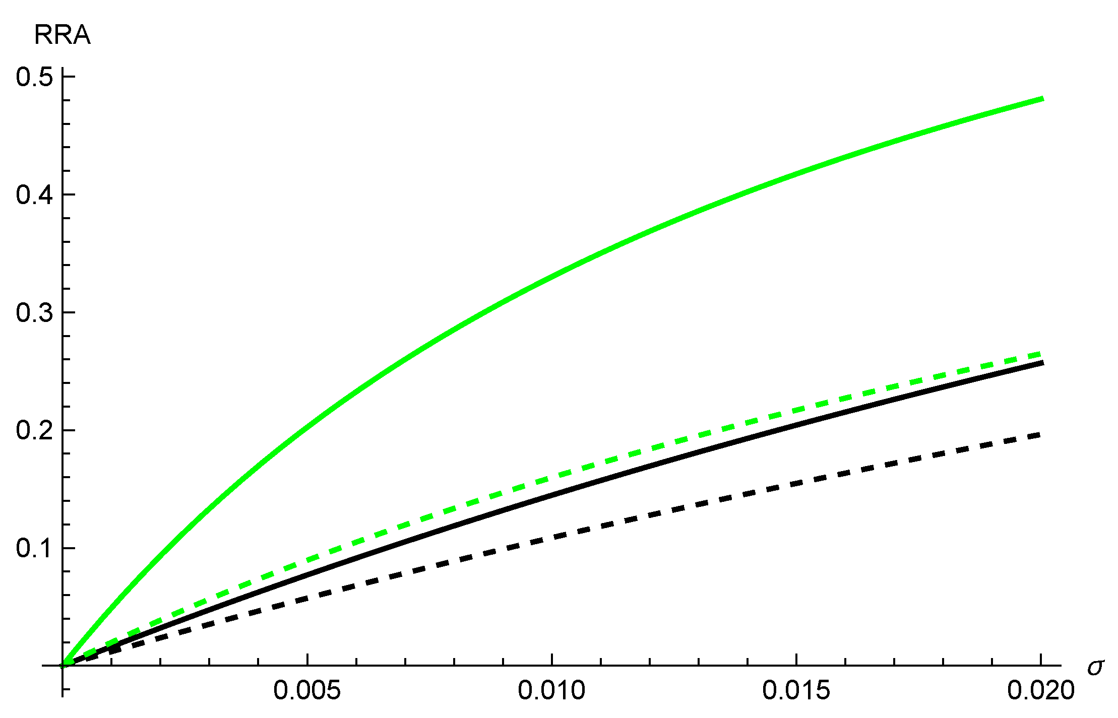
(c) Again, the argument of the exponential in ARA becomes more negative when increases. Hence ARA (and RRA) increases with . The RRA for different choices of r and T are plotted as a function of (Figure 8).
Here the green lines correspond to and the black lines to , further the dashed lines have and the solid lines have .
(d) and (e) These points are about parameter uncertainty. Our approach rests on two inputs, the best estimate r and the volatility . If we have short experience or another reason to consider these estimates uncertain, we can compensate by adding a margin to the risk adjustment. This shall not be seen as changing the chosen percentile, but rather to compensate for the fact that the true distribution might be wider than the calculated one.
6. Conclusions
This article presents one choice of approach for risk adjustment for surrender risk. It is based on a model calibrated to the company’s own data and hence is realistic. The risk adjustment is calculated by a method that is easy to program and which avoids time-consuming simulations. The final risk adjustment has reasonable properties, i.e., it fulfills the criteria in IFRS 17.
We believe that a similar approach can be used for some other non-financial risks, for example, mortality risk. Similarly to Solvency II, aggregation of risk adjustment for individual risk types becomes a question. A “Solvency II approach” with pre-defined correlations could be a solution, but obviously hard to justify. Still, it is difficult to see any alternatives, except a full simulation of the portfolio.
Funding
This research received no external funding.
Data Availability Statement
Data is unavailable due to confidentiality reasons.
Acknowledgments
The author thanks André Wong, Responsible for the Actuarial function at Swedbank Försäkring AB, and Lina Balčiūnienė, Actuary at Swedbank Life Insurance SE, who originally posed the questions leading to this work and who have provided valuable insight. The author also thanks Filip Lindskog, Stockholm University, for fruitful discussions. Finally, the anonymous referees made comments for which I am grateful and which have helped to improve the presentation.
Conflicts of Interest
The author declares no conflict of interest.
Appendix A. IFRS17 and Risk Adjustment for Non-Financial Risks
- “The key principles in IFRS 17 are that an entity:…(d) recognises and measures groups of insurance contracts at:(i) a risk-adjusted present value of the future cash flows (the fulfillment cash flows) that incorporates all of the available information about the fulfilment cash flows in a way that is consistent with observable market information; plus (if this value is a liability) or minus (if this value is an asset)(ii) an amount representing the unearned profit in the group of contracts (the contractual service margin).…”
In § 32, the fulfillment cash flow is defined:
- “...(i) estimates of future cash flows (§§ 33–35);(ii) an adjustment to reflect the time value of money and the financial risks related to the future cash flows, to the extent that the financial risks are not included in the estimates of the future cash flows (paragraph 36); and(iii) a risk adjustment for non-financial risk (§ 37).…”
The risk adjustment for non-financial risk is defined in § 37: “An entity shall adjust the estimate of the present value of the future cash flows to reflect the compensation that the entity requires for bearing the uncertainty about the amount and timing of the cash flows that arises from non-financial risk.”
In § 119, it is further stipulated: “An entity shall disclose the confidence level used to determine the risk adjustment for non-financial risk. If the entity uses a technique other than the confidence level technique for determining the risk adjustment for non-financial risk, it shall disclose the technique used and the confidence level corresponding to the results of that technique.”
| 1 | IFRS17 uses the sign convention that (discounted) claims and expenses are positive and (discounted) premiums negative. Here we reverse that, in order to look at it from the company’s point of view, and avoid a lot of minus signs. |
| 2 | For solvency purposes, more extreme events must be considered. Consequently, in Solvency II standard formula there is a capital requirement for “mass lapse” risk. |
| 3 | This subsection is courtesy of Lina Balčiūnienė. |
| 4 | For confidentiality reasons, the data has been modified. However, it has been done in a way that does not distort the statistical testing. |
| 5 | The Shapiro–Wilk test is tailored to test for normality based on the sample mean and sample variance. However, the specification of the sticky model has a fixed mean, and to be accurate, the Shapiro–Wilk test with a known mean should be used, see Hanusz et al. (2016) for details. The difference in our case is however negligible. |
| 6 | |
| 7 | For a good overview of approximation methods, see Asmussen et al. (n.d.). |
References
- Asmussen, Søren, Jens Ledet Jensen, and Leonardo Rojas-Nandayapa. n.d. A Literature Review on Log-Normal Sums. Available online: http://citeseerx.ist.psu.edu/viewdoc/summary?doi=10.1.1.719.5927 (accessed on 16 March 2023).
- Barsotti, Flavia, Xavier Milhaud, and Yahia Salhi. n.d. Lapse Risk in Life Insurance: Correlation and Contagion Effects among Policyholders’ Behaviors. Available online: https://hal.archives-ouvertes.fr/hal-01282601v2 (accessed on 16 March 2023).
- Boumezoud, Alexandre, Amal Elfassihi, Cormac Gleeson, Andrew Kay, Orlaith Lehana, Bertrand Lespinasse, and Damien Louvet. 2020. IFRS 17: Deriving the Confidence Level for the Risk Adjustment: A Case Study for Life (re)Insurers. Paris: Milliman. Available online: https://www.milliman.com/en/insight/IFRS-17-Deriving-the-confidence-level-for-the-Risk-Adjustment-A-case-study-for-life-reinsurers (accessed on 16 March 2023).
- Chaoubi, Ihsan, Hélène Cossette, Simon-Pierre Gadoury, and Etienne Marceau. 2020. On sums of two counter-monotonic risks. Insurance: Mathematics and Economics 92: 47–60. [Google Scholar] [CrossRef]
- Deelstra, Griselda, Ibrahima Diallo, and Michèle Vanmaele. 2008. Bounds for Asian basket options. Journal of Computational and Applied Mathematics 218: 215–28. [Google Scholar] [CrossRef] [Green Version]
- Denuit, Michel, Jan Dhaene, Marc Goovaerts, and Rob Kaas. 2005. Actuarial Theory for Dependent Risk: Measures, Orders and Models. New York: Wiley. [Google Scholar]
- Dhaene, Jan, Steven Vanduffel, Marc Goovaerts, Rob Kaas, Qihe Tang, and David Vyncke. 2006. Risk measures and comonotonicity: A review. Stochastic Models 22: 573–606. [Google Scholar] [CrossRef] [Green Version]
- Eling, Martin, and Michael Kochanski. 2013. Research on lapse in life insurance: What has been done and what needs to be done? The Journal of Risk Finance 14: 392–413. [Google Scholar] [CrossRef] [Green Version]
- England, Peter D., Richard J. Verrall, and Mario Valentin Wüthrich. 2019. On the lifetime and one-year views of reserve risk, with application to IFRS 17 and Solvency II risk margins. Insurance: Mathematics and Economics 85: 74–88. [Google Scholar] [CrossRef]
- Grandell, Jan. 1991. Aspects of Risk Theory. Springer Series in Statistics. Probability and Its Applications; New York: Springer. [Google Scholar]
- Hanbali, Hamza, and Daniel Linders. 2019. American-type basket option pricing: A simple two-dimensional partial differential equation. Quantitative Finance 19: 1689–704. [Google Scholar] [CrossRef]
- Hanbali, Hamza, Daniël Linders, and Jan Dhaene. 2022. Value-at-Risk, Tail Value-at-Risk and upper tail transform of the sum of two counter-monotonic random variables. Scandinavian Actuarial Journal 2023: 219–43. [Google Scholar] [CrossRef]
- Hanusz, Zofia, Joanna Tarasinska, and Wojciech Zielinski. 2016. Shapiro–Wilk test with known mean. Revstat Statistical Journal 14: 89–100. [Google Scholar]
- Hesselager, Ole. 1993. Extensions to Ohlin’s lemma with applications to optimal reinsurance structures. Insurance: Mathematics and Economics 13: 83–97. [Google Scholar] [CrossRef]
- IAA. 2018. Risk Adjustments for Insurance Contracts under IFRS 17. Monograph. Ottawa: International Actuarial Association. [Google Scholar]
- IFRS 17 Insurance Contracts. n.d. International Accounting Standards Board. Available online: https://www.ifrs.org/issued-standards/list-of-standards/ifrs-17-insurance-contracts.html/content/dam/ifrs/publications/html-standards/english/2023/issued/ifrs17/ (accessed on 16 March 2023).
- Kaas, Rob, Jan Dhaene, and Marc J. Goovaerts. 2000. Upper and lower bounds for sums of random variables. Insurance: Mathematics and Economics 27: 151–68. [Google Scholar] [CrossRef] [Green Version]
- Linders, Daniël, and Ben Stassen. 2016. The multivariate Variance Gamma model: Basket option pricing and calibration. Quantitative Finance 16: 555–72. [Google Scholar] [CrossRef]
- Milhaud, Xavier, and Christophe Dutang. 2018. Lapse tables for lapse risk management in insurance: A competing risk approach. European Actuarial Journal 8: 97–126. [Google Scholar] [CrossRef] [Green Version]
- Ohlin, Jan. 1969. On a class of measures of dispersion with application to optimal reinsurance. Astin Bulletin 5: 249–66. [Google Scholar] [CrossRef] [Green Version]
- Palmborg, Lina, Mathias Lindholm, and Filip Lindskog. 2021. Financial position and performance in IFRS 17. Scandinavian Actuarial Journal 3: 171–97. [Google Scholar] [CrossRef]
- Smith, William, Jennifer Strickland, Ed Morgan, and Marcin Krzykowski. 2019. 2018 IFRS 17 Preparedness Survey. London: Milliman. Available online: https://www.milliman.com/en/insight/2018-IFRS-Preparedness-Survey (accessed on 16 March 2023).
Figure 1.
Remain rate of four portfolios over time.

Figure 2.
Lognormal model: simulated paths of cash flows.

Figure 3.
Sticky model: simulated paths of cash flows.

Figure 4.
Quantile function of the total portfolio value for different p.

Figure 5.
20% (blue) and 80% (orange) quantile of the cash flow in each time point t.

Figure 6.
Quantile function of S (thick green), (blue), and (orange), for different p.

Figure 7.
Partial expectation of S (thick green), (blue), and (orange), for different p.

Figure 8.
Relative risk adjustment as a function of .

Disclaimer/Publisher’s Note: The statements, opinions and data contained in all publications are solely those of the individual author(s) and contributor(s) and not of MDPI and/or the editor(s). MDPI and/or the editor(s) disclaim responsibility for any injury to people or property resulting from any ideas, methods, instructions or products referred to in the content. |
© 2023 by the author. Licensee MDPI, Basel, Switzerland. This article is an open access article distributed under the terms and conditions of the Creative Commons Attribution (CC BY) license (https://creativecommons.org/licenses/by/4.0/).
Share and Cite
MDPI and ACS Style
Carlehed, M. A Model for Risk Adjustment (IFRS 17) for Surrender Risk in Life Insurance. Risks 2023, 11, 62. https://doi.org/10.3390/risks11030062
AMA Style
Carlehed M. A Model for Risk Adjustment (IFRS 17) for Surrender Risk in Life Insurance. Risks. 2023; 11(3):62. https://doi.org/10.3390/risks11030062
Chicago/Turabian StyleCarlehed, Magnus. 2023. "A Model for Risk Adjustment (IFRS 17) for Surrender Risk in Life Insurance" Risks 11, no. 3: 62. https://doi.org/10.3390/risks11030062
Note that from the first issue of 2016, this journal uses article numbers instead of page numbers. See further details here.