
Auxiliary Segmentation Method of Osteosarcoma in MRI Images Based on Denoising and Local Enhancement


Abstract
:1. Introduction
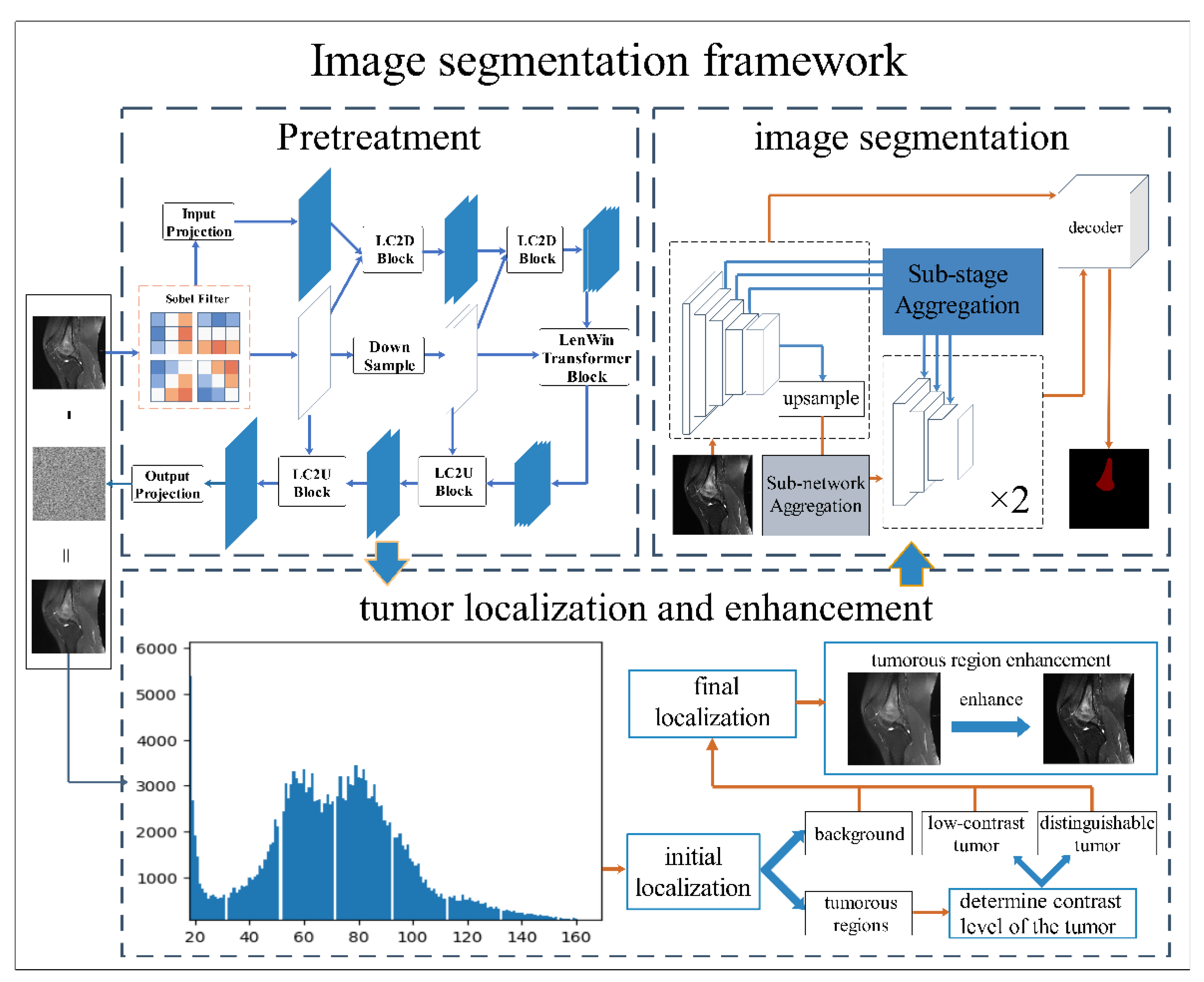
- This study proposes an auxiliary segmentation method of osteosarcoma in MRI images based on denoising and local enhancement, improving the accuracy and speed of segmentation and reducing resource consumption.
- We use the medical denoising model Eformer to remove noise and then localize and enhance the osteosarcoma region in MRI images. After preprocessing, the tumor region in the MRI image will be clearer and the boundary can be enhanced. Finally, an efficient and accurate network DFANet is used to segment osteosarcoma in MRI images.
2. Related Works
3. Methods
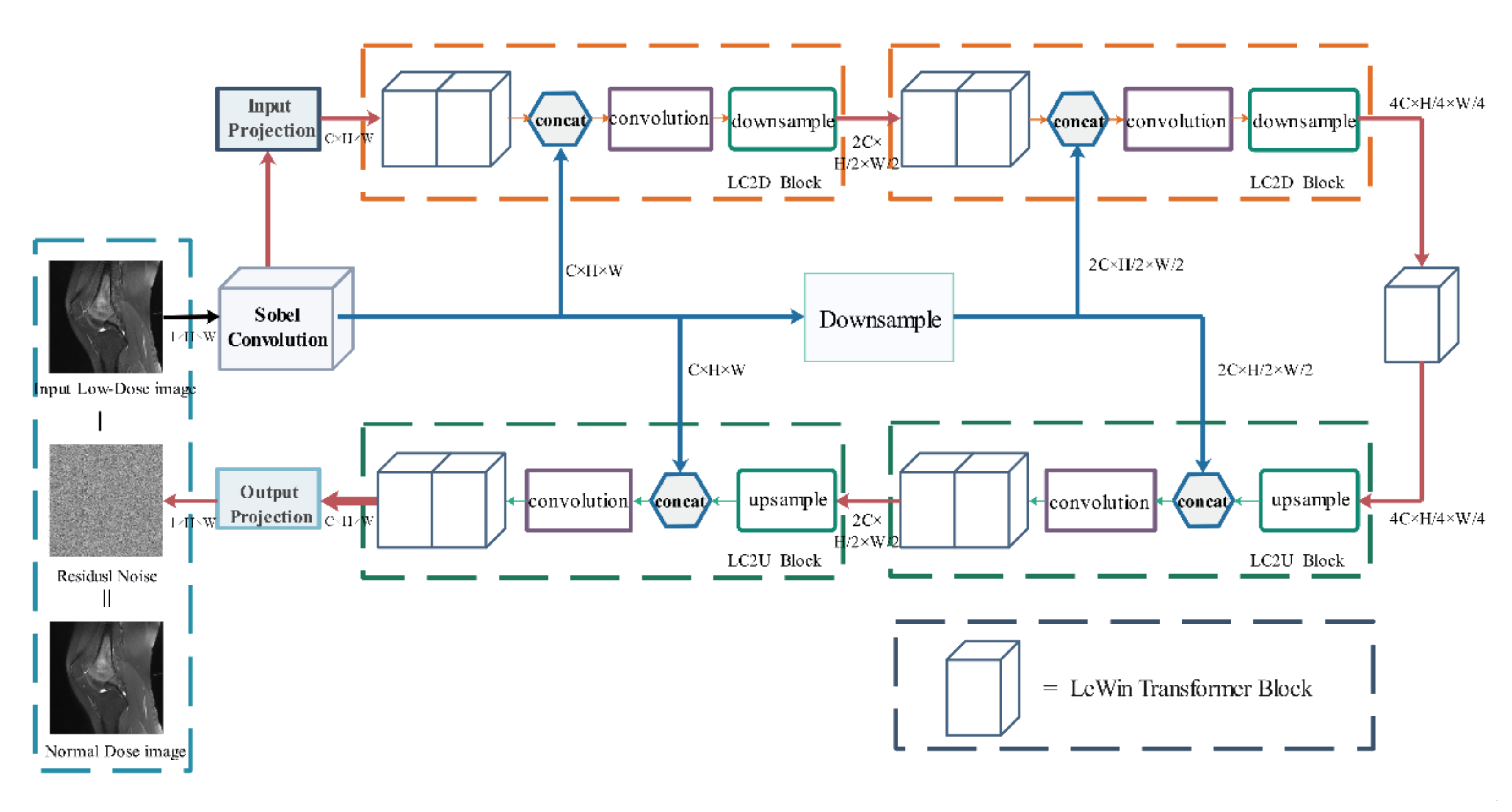
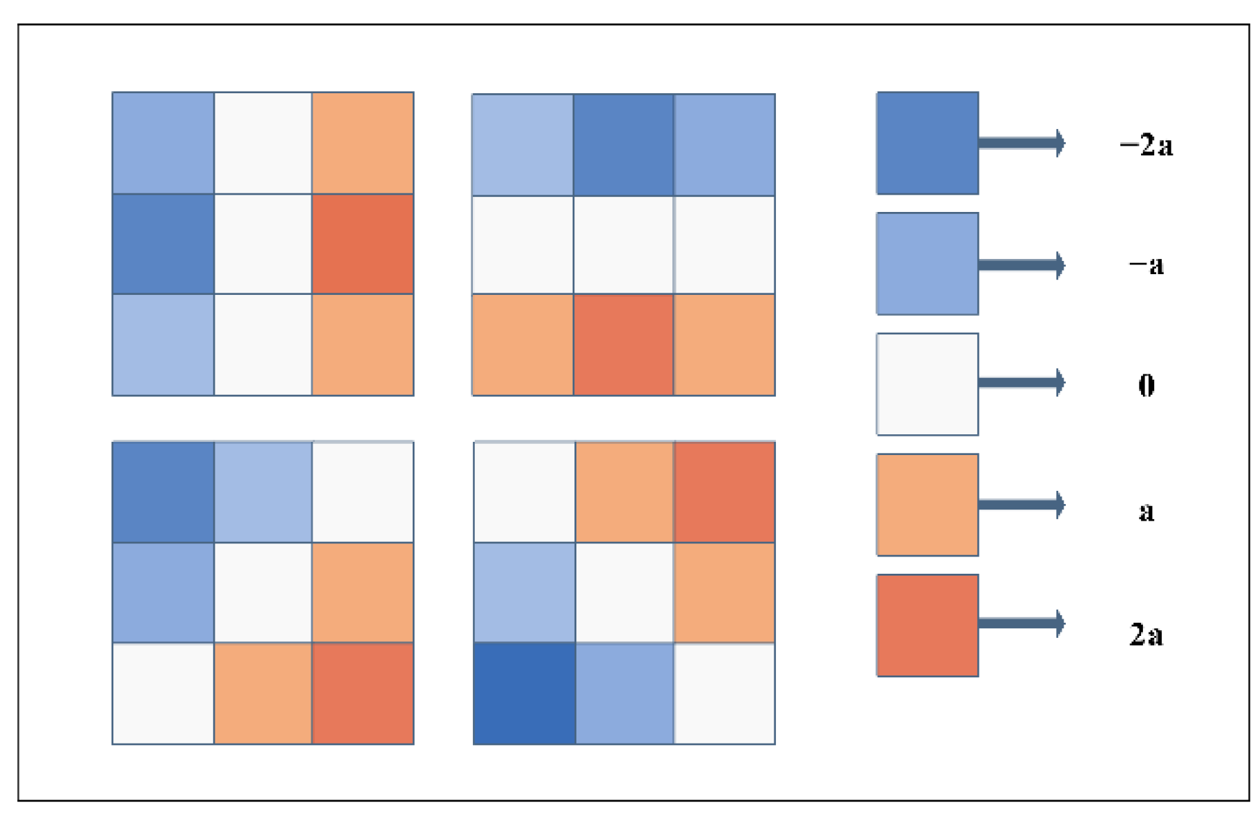
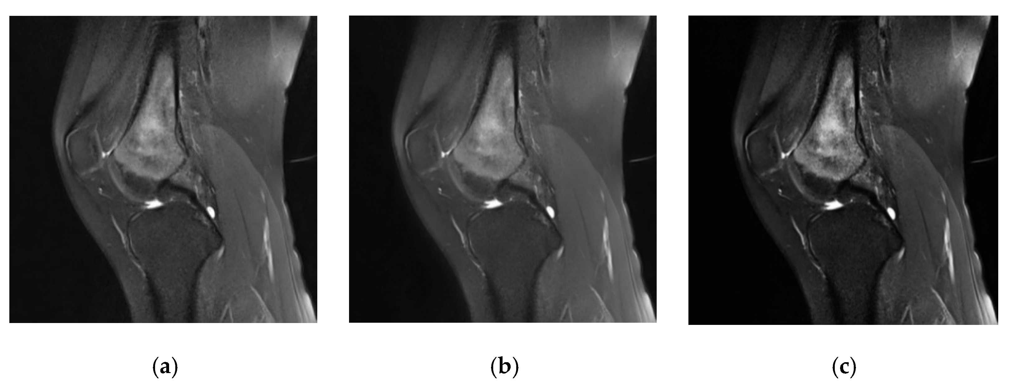
3.1. Remove Noise
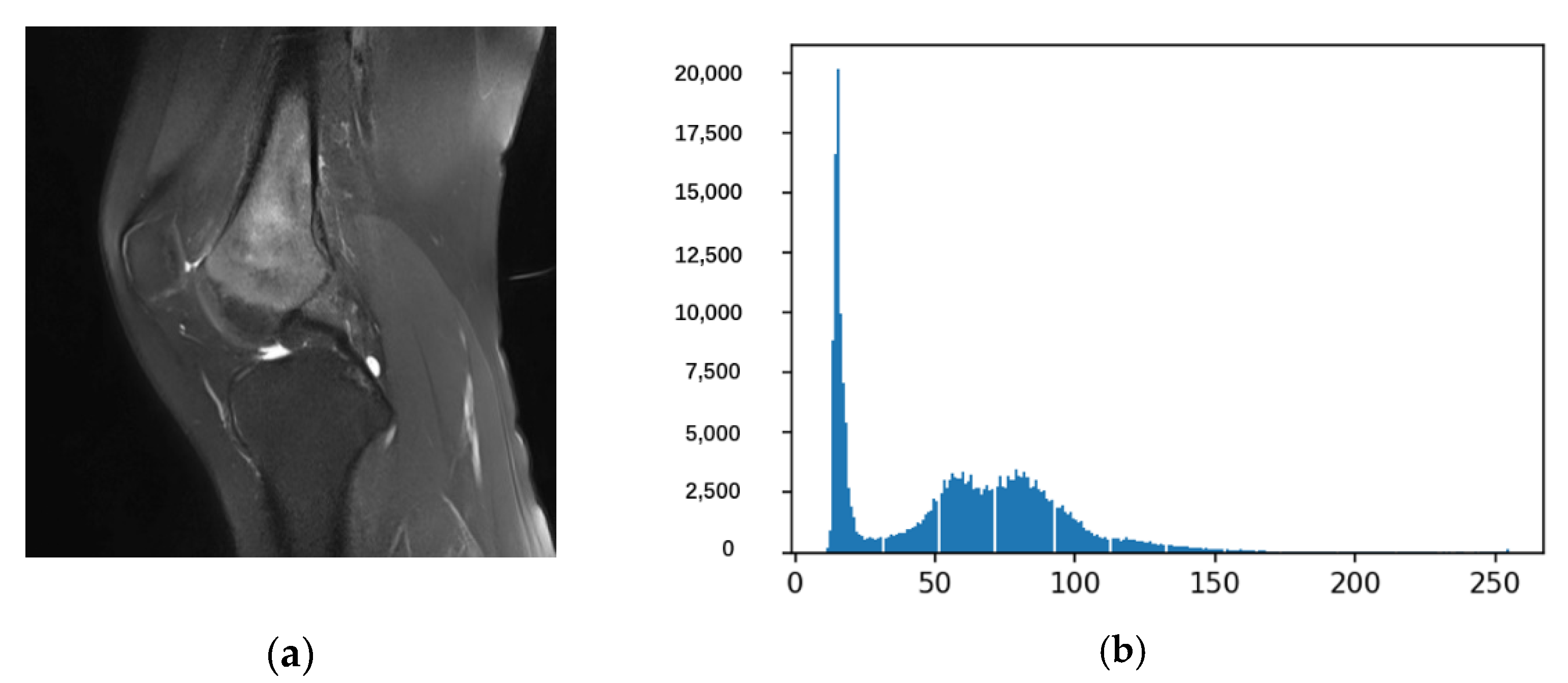
3.2. Tumor Localization and Enhancement Methods
3.3. Osteosarcoma Image Segmentation
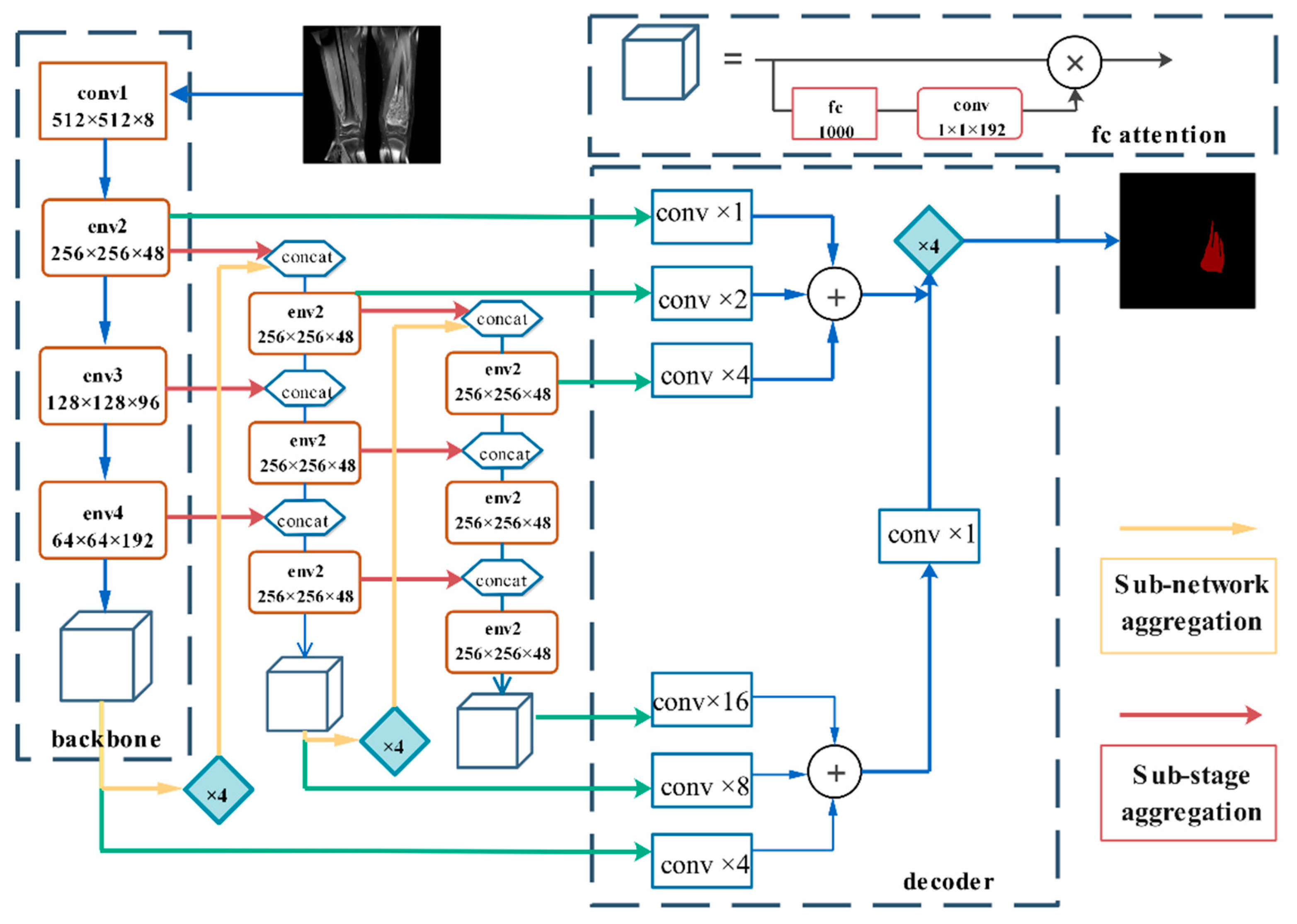
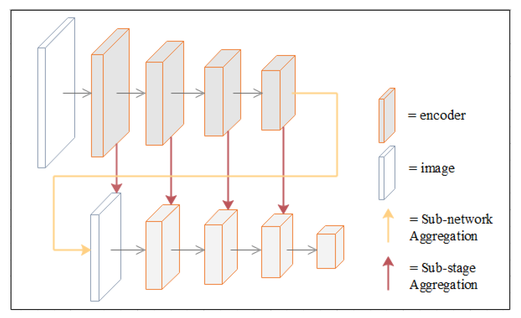
3.3.1. Deep Feature Aggregation Network (DFANet)
3.3.2. Network Architecture
3.3.3. Deep Feature Aggregation
4. Experiments
4.1. Dataset
4.2. Evaluation Indicators
4.3. Comparison Algorithm
4.4. Parameter Setting
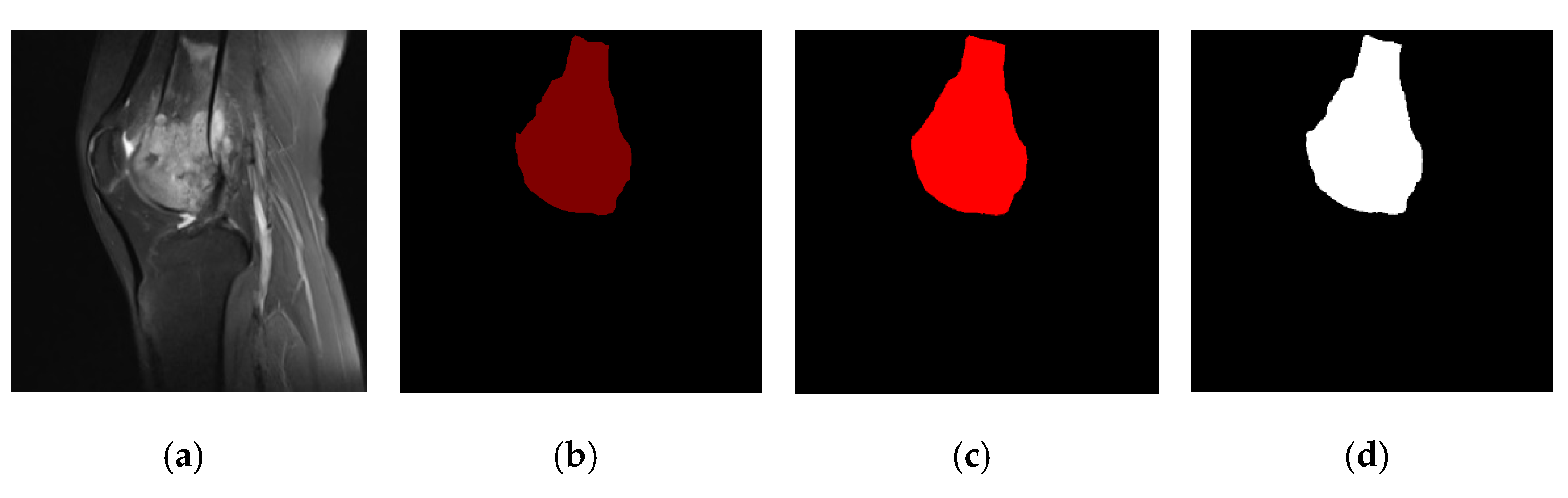
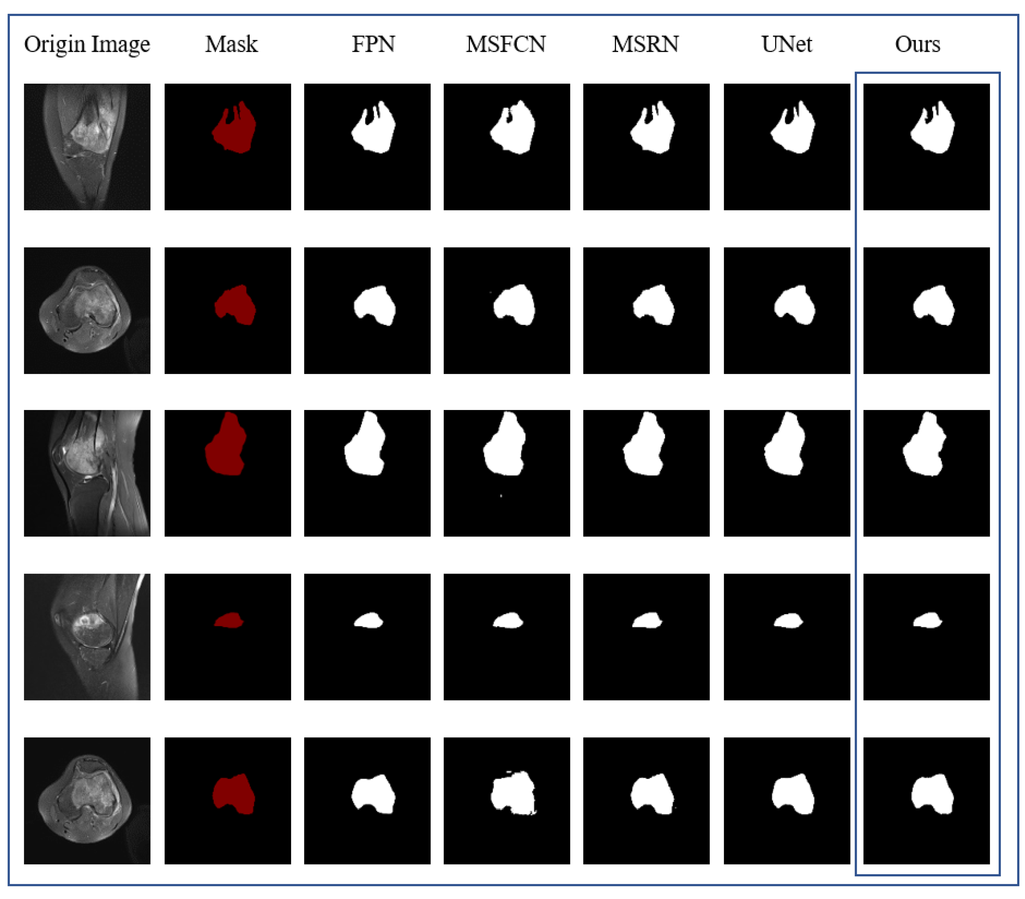
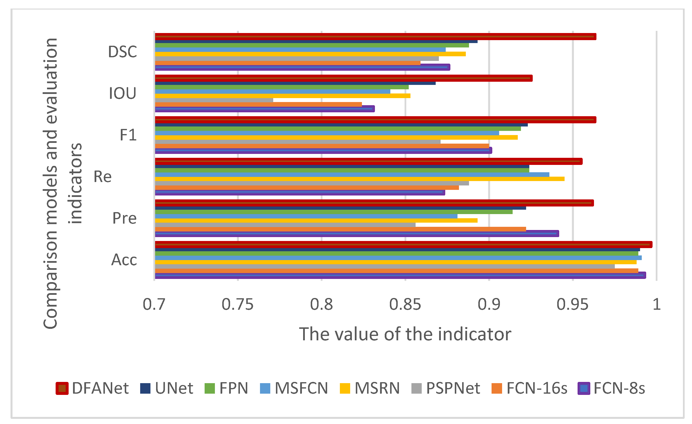
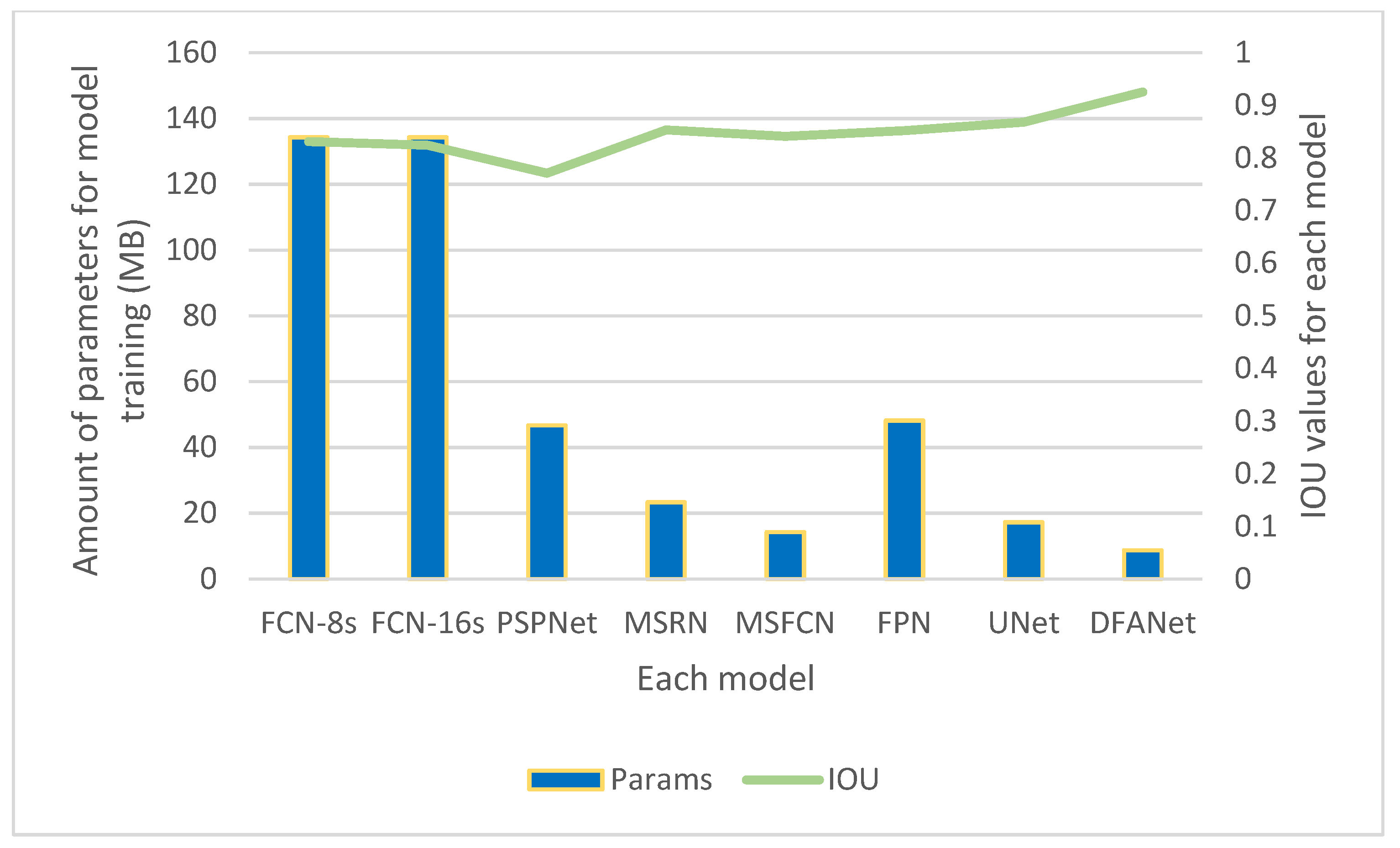
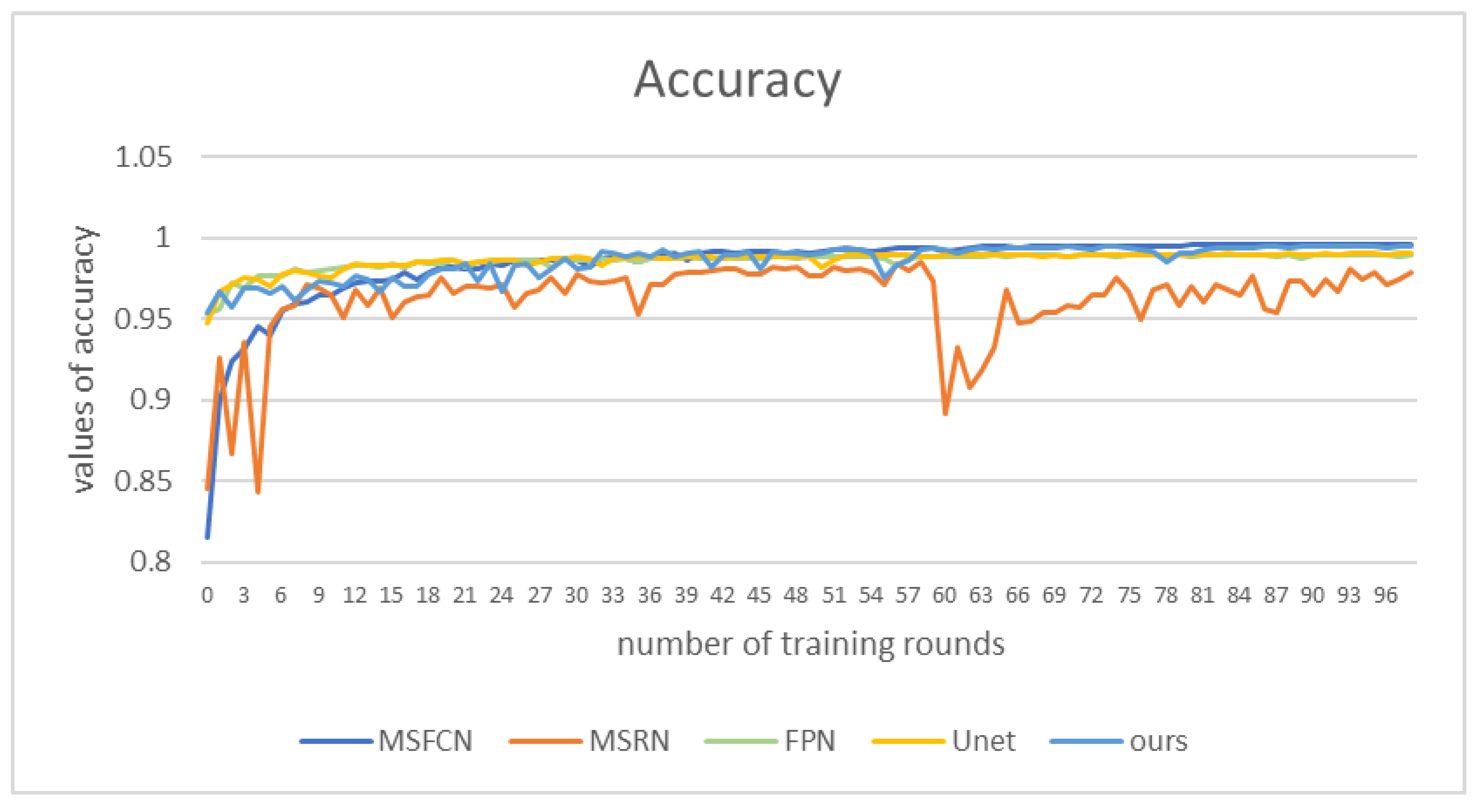
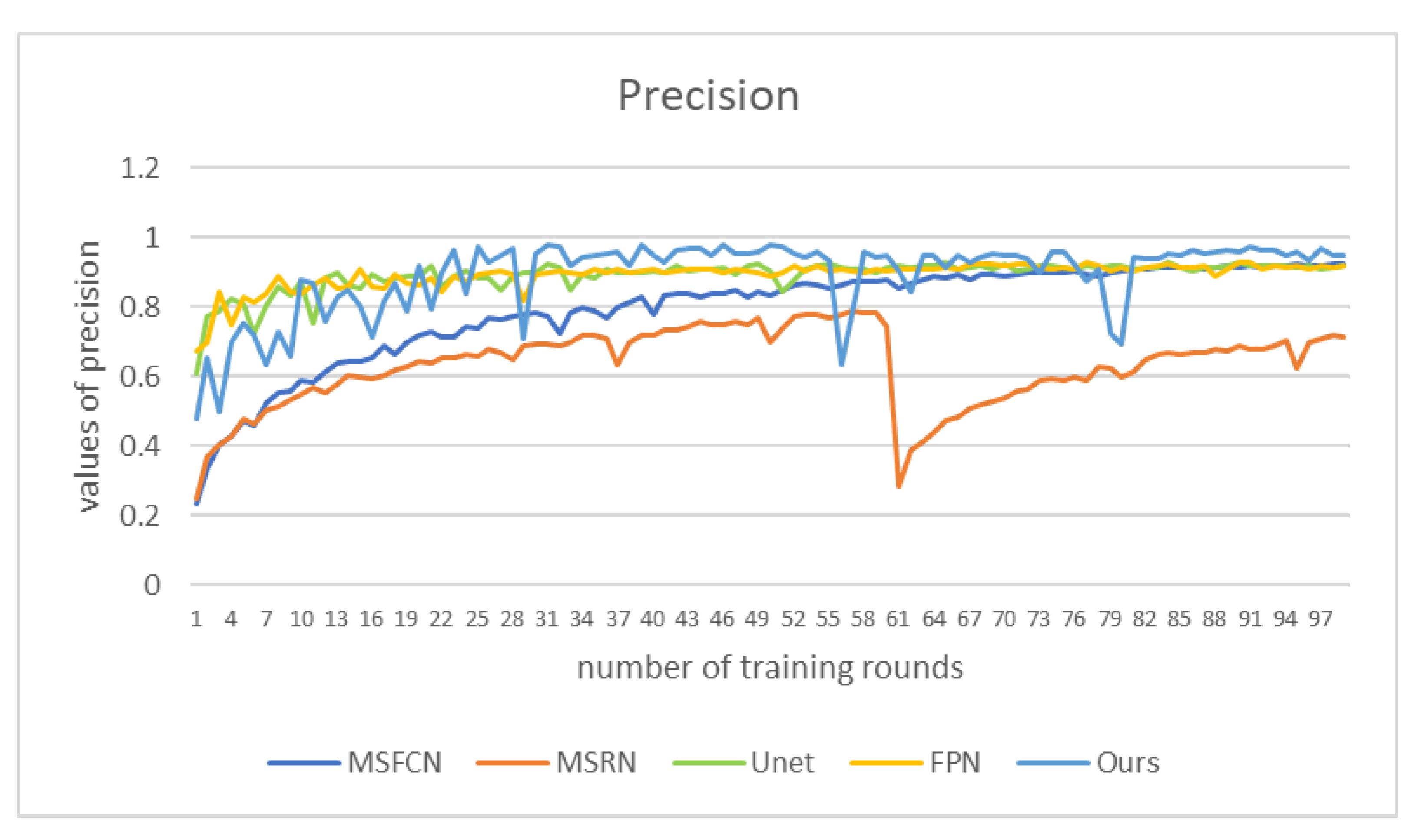
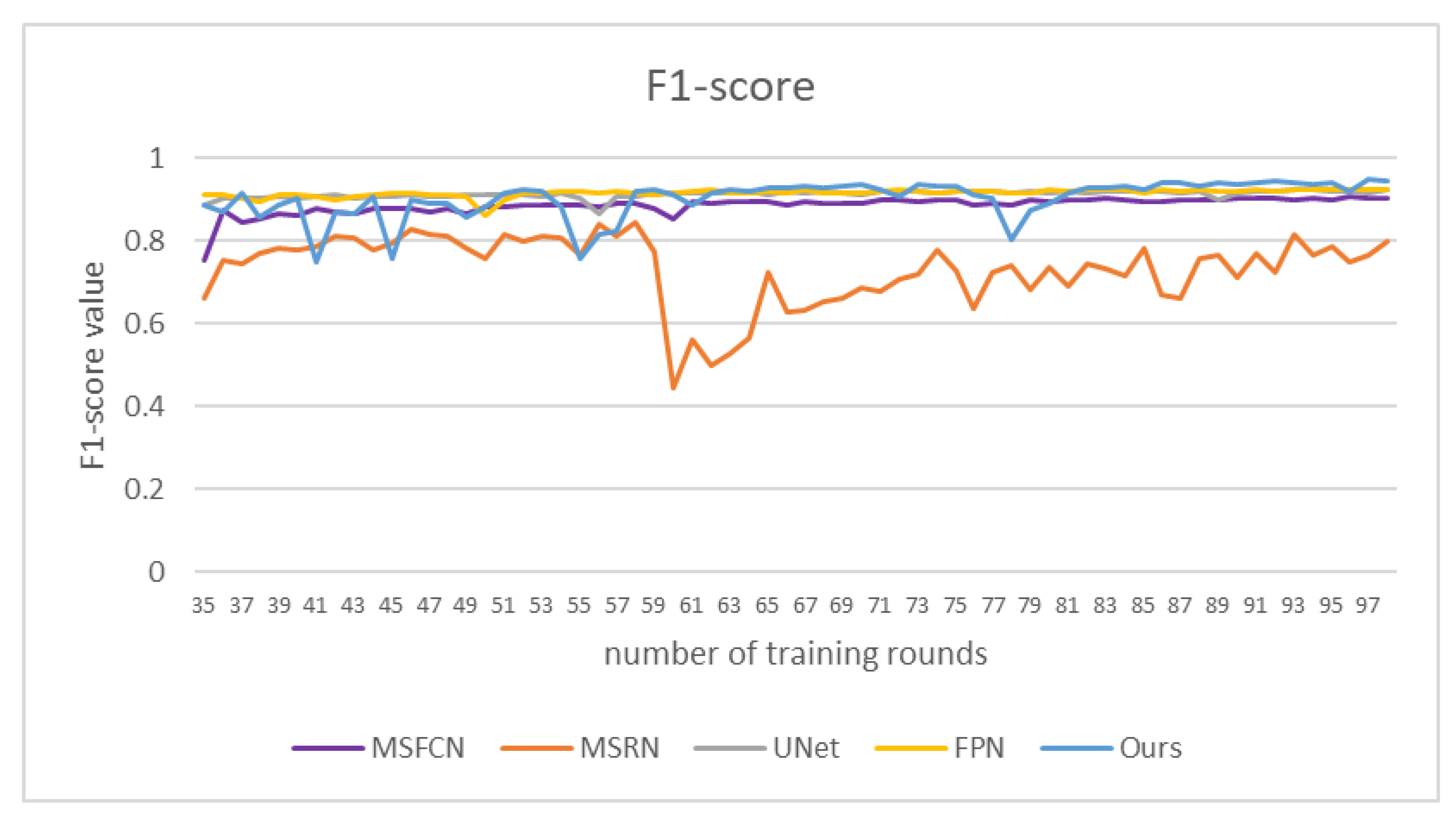
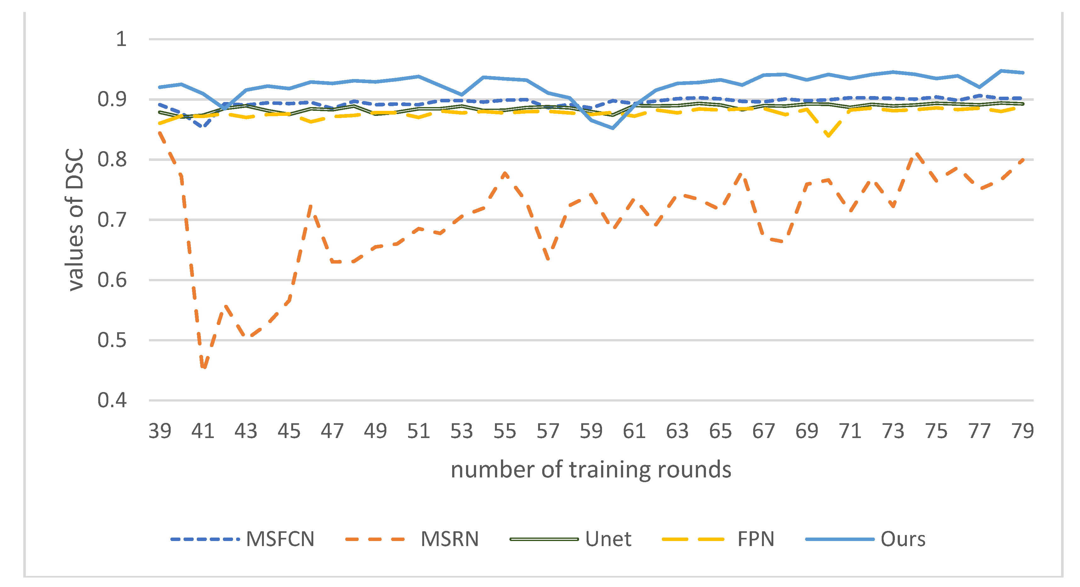
4.5. Evaluation of Segmentation Effect
5. Summary
Author Contributions
Funding
Institutional Review Board Statement
Informed Consent Statement
Data Availability Statement
Acknowledgments
Conflicts of Interest
References
- Corre, I.; Verrecchia, F.; Crenn, V.; Redini, F.; Trichet, V. The Osteosarcoma Microenvironment: A Complex but Targetable Ecosystem. Cells 2020, 9, 976. [Google Scholar] [CrossRef] [PubMed] [Green Version]
- Liu, F.; Gou, F.; Wu, J. An Attention-Preserving Network-Based Method for Assisted Segmentation of Osteosarcoma MRI Images. Mathematics 2022, 10, 1665. [Google Scholar] [CrossRef]
- Kazuhiro, T.; Toshifumi, O. Management of elderly patients with bone and soft tissue sarcomas: JCOG Bone and Soft Tissue Tumor Study Group. Jpn. J. Clin. Oncol. 2022, 52, 526–530. [Google Scholar]
- Le, T.; Su, S.; Shahriyari, L. Immune classification of osteosarcoma. Math. Biosci. Eng. 2021, 18, 1879–1897. [Google Scholar] [CrossRef] [PubMed]
- Liu, Z.; Zhou, X.; Xiong, W. BA-GCA Net: Boundary Aware Grid Contextual Attention Net in Osteosarcoma MRI Image Segmentation. Comput. Intell. Neurosci. 2022, 2022, 3881833. [Google Scholar] [CrossRef]
- Xiao, P.; Zhou, Z.; Dai, Z. An artificial intelligence multiprocessing scheme for the diagnosis of osteosarcoma MRI images. IEEE J. Biomed. Health Inform. 2021, 15, 1–12. [Google Scholar] [CrossRef]
- Arianna, F.; Gasperini, C.; Gómez, M.P.A.; Bazzocchi, A.; Fanti, S.; Nanni, C. The Role of FDG-PET and Whole-Body MRI in High Grade Bone Sarcomas with Particular Focus on Osteosarcoma; WB Saunders: Philadelphia, PA, USA, 2021. [Google Scholar]
- Abd, A.R.H.; Gaber, K.M.M.; Ahmed, A.I. Role of Diffusion Weighted MRI in Assessment of Treatment Response to Chemotherapy in Patients with Osteogenic Sarcoma. QJM Int. J. Med. 2021, 114 (Suppl. S1). [Google Scholar]
- Chen, H.; Liu, J.; Cheng, Z.; Lu, X.; Wang, X.; Lu, M.; Li, S.; Xiang, Z.; Zhou, Q.; Liu, Z.; et al. Development and external validation of an MRI-based radiomics nomogram for pretreatment prediction for early relapse in osteosarcoma: A retrospective multicenter study. Eur. J. Radiol. 2020, 129, 109066. [Google Scholar] [CrossRef]
- Zhuang, Q.; Dai, Z. Deep active learning framework for lymph nodes metastases prediction in medical support system. Comput. Intell. Neurosci. 2022, 2022, 4601696. [Google Scholar] [CrossRef]
- Tian, X.; Yan, L.; Jiang, L. Comparative transcriptome analysis of leaf, stem, and root tissues of Semiliquidambar cathayensis reveals candidate genes involved in terpenoid biosynthesis. Mol. Biol. Rep. 2022, 49, 5585–5593. [Google Scholar] [CrossRef]
- Kayal, E.B.; Kandasamy, D.; Sharma, R.; Bakhshi, S.; Mehndiratta, A. Segmentation of osteosarcoma tumor using diffusion weighted MRI: A comparative study using nine segmentation algorithms. Signal Image Video Process. 2020, 14, 727–735. [Google Scholar] [CrossRef]
- Yang, S.; Zhou, Z.; Xie, P.; Xu, N.; Dai, Z. Intelligent Segmentation Medical Assistance System for MRI Images of osteosarcoma in Developing Countries. Comput. Math. Methods Med. 2022, 2022, 6654946. [Google Scholar] [CrossRef]
- Yu, G.; Chen, Z.; Tan, Y. Medical Decision Support System for Cancer Treatment in Precision Medicine in Developing Countries. Expert Syst. Appl. 2021, 186, 115725. [Google Scholar] [CrossRef]
- Jia, W.; Gou, F.; Tan, Y.A. Staging Auxiliary Diagnosis Model for Nonsmall Cell Lung Cancer Based on the 707 Intelligent Medical System. Comput. Math. Methods Med. 2021, 2021, 6654946. [Google Scholar] [CrossRef]
- Shen, Y.; Gou, F.; Dai, Z. Osteosarcoma MRI Image-Assisted Segmentation System Base on Guided Aggregated Bilateral Network. Mathematics 2022, 10, 1090. [Google Scholar] [CrossRef]
- Yu, G.; Wu, J. Efficacy prediction based on attribute and multi-source data collaborative for auxiliary medical system in developing countries. Neural Comput. Appl. 2022, 34, 5497–5512. [Google Scholar] [CrossRef]
- Chang, L.; Yu, G. Effective Data Decision-Making and Transmission System Based on Mobile Health for Chronic Disease Management in the Elderly. IEEE Syst. J. 2021, 15, 5537–5548. [Google Scholar] [CrossRef]
- Qin, Y.; Li, X. A management method of chronic diseases in the elderly based on IoT security environment. Comput. Electr. Eng. 2022, 102, 108188. [Google Scholar] [CrossRef]
- Jiao, Y.; Qi, H. Capsule network assisted electrocardiogram classification model for smart healthcare. Biocybern. Biomed. Eng. 2022, 42, 543–555. [Google Scholar] [CrossRef]
- Fangfang, G.; Wu, J. Data Transmission Strategy Based on Node Motion Prediction IoT System in Opportunistic Social Networks. Wirel. Pers. Commun. 2022, 121, 1–12. [Google Scholar] [CrossRef]
- Krm, F.; Tsokos, C.P. Deep and Statistical Learning in Biomedical Imaging: State of the Art in 3D MRI Brain Tumor Segmentation. arXiv 2021, arXiv:2103.05529. [Google Scholar]
- Xiong, W.; Zhou, X. A Reputation Value-based Task-sharing Strategy in Opportunistic Complex Social Networks. Complexity 2021, 2021, 8554351. [Google Scholar] [CrossRef]
- Amin, J.; Sharif, M.; Raza, M.; Saba, T.; Anjum, M.A. Brain tumor detection using statistical and machine learning method. Comput. Methods Programs Biomed. 2019, 177, 69–79. [Google Scholar] [CrossRef]
- Chang, L.; Moustafa, N.; Bashir, A.K.; Yu, K. AI-Driven Synthetic Biology for Non-Small Cell Lung Cancer Drug Effectiveness-Cost Analysis in Intelligent Assisted Medical Systems. IEEE J. Biomed. Health Inform. 2021, 54, 1–12. [Google Scholar] [CrossRef]
- Ouyang, T.; Yang, S.; Dai, Z. Rethinking U-Net from an Attention Perspective with Transformers for Osteosarcoma MRI Image Segmentation. Comput. Intell. Neurosci. 2022, 2022, 7973404. [Google Scholar] [CrossRef]
- Norouzi, A.; Shafry, M.; Rahim, M.; Altameem, A.; Saba, T.; Rad, A.E.; Rehman, A.; Uddin, M. Applications medical image segmentation methods, algorithms, and applications. IETE Tech. Rev. 2014, 3, 37–41. [Google Scholar] [CrossRef]
- Li, L.; Gou, F.; Long, H.; He, K.; Wu, J. Effective data optimization and evaluation based on social communication with AI-assisted in opportunistic social networks. Wirel. Commun. Mob. Comput. 2022, 2022, 4879557. [Google Scholar] [CrossRef]
- Mandava, R.; Wei, B.C.; Yeow, L.S. Spatial multiple criteria fuzzy clustering for image segmentation. In Proceedings of the Second International Conference on Computational Intelligence, Washington, DC, USA, 28–30 September 2010; IEEE: Manhattan, NY, USA, 2010; pp. 305–310. [Google Scholar]
- Ebk, A.; Kandasamy, D.; Yadav, R.; Bakhshi, S.; Sharma, R.; Mehndiratta, A. Automatic segmentation and RECIST score evaluation in osteosarcoma using diffusion MRI: A computer aided system process. Eur. J. Radiol. 2020, 133, 109359. [Google Scholar]
- Frangi, A.F.; Egmont-Petersen, M.; Niessen, W.J.; Reiber, J.H.C.; Viergever, M.A. Bone tumor segmentation from MR perfusion images with neural networks using multi-scale pharmacokinetic features. Image Vis. Comput. 2001, 19, 679–690. [Google Scholar] [CrossRef]
- Glass, J.O.; Reddick, W.E. Hybrid artificial neural network segmentation and classification of dynamic contrast-enhanced MR imaging (DEMRI) of osteosarcoma. Magn. Reson. Imaging 1998, 16, 1075–1083. [Google Scholar] [CrossRef]
- CHEN, C.X.; Zhang, D.; Li, N.; Qian, X.J.; Wu, S.; Gail, S. Osteosarcoma segmentation in MRI based on Zernike moment and SVM. Chin. J. Biomed. Eng. 2013, 22, 70–78. [Google Scholar]
- Tripathy, R.; Bilionis, I.; Gonzalez, M. Gaussian processes with built-in dimen sionality reduction: Applications to high-dimensional uncertainty propagation. J. Comput. Phys. 2016, 321, 191–223. [Google Scholar] [CrossRef] [Green Version]
- Zhang, X.; Mei, C.L.; Chen, D.G.; Li, J.H. Feature selection in mixed data: A method using a novel fuzzy rough set-based information entropy. Pattern Recognit. 2016, 56, 1–15. [Google Scholar] [CrossRef]
- Mohammad, H.; Davy, A.; Warde-Farley, D.; Biard, A.; Courville, A.; Bengio, Y.; Pal, C.; Jodoin, P.; Larochelle, H. Brain tumor segmentation with deep neural networks. Med. Image Anal. 2016, 35, 18–31. [Google Scholar]
- Rui, Z.; Huang, L.; Xia, W.; Zhang, B.; Qiu, B.; Gao, X. Multiple supervised residual network for osteosarcoma segmentation in CT images. Comput. Med. Imaging Graph. 2018, 63, 1–8. [Google Scholar]
- Barzekar, H.; Yu, Z. C-Net: A Reliable Convolutional Neural Network for Biomedical Image Classification. 2022, 187, 116003. Expert Syst. Appl. 2022, 187, 116003. [Google Scholar] [CrossRef]
- Anisuzzaman, D.M.; Barzekar, H.; Tong, L.; Luo, J.; Yu, Z. A deep learning study on osteosarcoma detection from histological images. Biomed. Signal Process. Control 2021, 69, 102931. [Google Scholar] [CrossRef]
- Isensee, F.; Jaeger, P.F.; Kohl, S.A.; Petersen, J.; Maier-Hein, K.H. nnU-Net: A self-configuring method for deep learning-based biomedical image segmentation. Nat. Methods 2021, 18, 203–211. [Google Scholar] [CrossRef]
- Bengio, Y.; Courville, A.; Vincent, P. Representation Learning: A Review and New Perspectives. IEEE Trans. Pattern Anal. Mach. Intell. 2013, 35, 1798–1828. [Google Scholar] [CrossRef]
- Fangfang, G.; Wu, J. Message transmission strategy based on recurrent neural network and attention mechanism in IoT system. J. Circuits Syst. Comput. 2022, 31, 2250126. [Google Scholar] [CrossRef]
- Xie, S.; Tu, Z. Holistically-nested edge detection. In Proceedings of the IEEE International Conference on Computer Vision, Santiago, Chile, 7–16 December 2015; pp. 1395–1403. [Google Scholar]
- Cui, R.; Chen, Z.; Tan, Y.; Yu, G. A Multiprocessing Scheme for PET Image Pre-Screening, Noise Reduction, Segmentation and Lesion Partitioning. IEEE J. Biomed. Health Inform. 2021, 25, 1699–1711. [Google Scholar] [CrossRef]
- Yu, G.; Chen, Z.; Tan, Y. A Diagnostic Prediction Framework on Auxiliary Medical System for Breast Cancer in Developing Countries. Knowl. -Based Syst. 2021, 232, 107459. [Google Scholar] [CrossRef]
- Jia, W.; Xia, J.; Gou, F. Information transmission mode and IoT community reconstruction based on user influence in opportunistic social networks. Peer-to-Peer Netw. Appl. 2022, 15, 1398–1416. [Google Scholar] [CrossRef]
- Yang, W.; Luo, J. Application of information transmission control strategy based on incremental community division in IoT platform. IEEE Sens. J. 2021, 21, 21968–21978. [Google Scholar] [CrossRef]
- Tian, X.; Wu, J.; Gou, F. Disease Control and Prevention in Rare Plants Based on the Dominant Population Selection Method in Opportunistic Social Networks. Comput. Intell. Neurosci. 2022, 2022, 1489988. [Google Scholar] [CrossRef]
- Sobel, I. An Isotropic 3 × 3 Image Gradient Operator. Presented at Stanford A.I. Project 1968, San Francisco, CA, USA, 2 February, 2014.
- Yepeng, D.; Gou, F.; Wu, J. Hybrid Data Transmission Scheme Based on Source Node Centrality and Community Reconstruction in Opportunistic Social Network. Peer-to-Peer Netw. Appl. 2021, 14, 3460–3472. [Google Scholar] [CrossRef]
- Liang, T.; Jin, Y.; Li, Y.; Wang, T. Edcnn: Edge enhancement-based densely connected network with compound loss for low-dose ct denoising. In Proceedings of the 2020 15th IEEE International Conference on Signal Processing (ICSP), Beijing, China, 6–9 December 2020; IEEE: Manhattan, NY, USA, 2020. [Google Scholar]
- Ilhan, A.; Sekeroglu, B.; Abiyev, R. Brain tumor segmentation in MRI images using non-parametric localization and enhancement methods with U-net. Int. J. Comput. Assist. Radiol. Surg. 2022, 17, 589–600. [Google Scholar] [CrossRef]
- Li, H.; Xiong, P.; Fan, H.; Sun, J. DFANet: Deep Feature Aggregation for Real-Time Semantic Segmentation. In Proceedings of the 2019 IEEE/CVF Conference on Computer Vision and Pattern Recognition (CVPR), Long Beach, CA, USA, 15–20 June 2019; pp. 9514–9523. [Google Scholar] [CrossRef] [Green Version]
- Gou, F.; Wu, J. Triad link prediction method based on the evolutionary analysis with IoT in opportunistic social networks. Comput. Commun. 2022, 181, 143–155. [Google Scholar] [CrossRef]
- Xiangbing, Z.; Long, H.; Duan, X.; Kong, G. A Convolutional Neural Network-Based Intelligent Medical System with Sensors for Assistive Diagnosis and Decision-Making in Non-Small Cell Lung Cancer. Sensors 2021, 21, 7996. [Google Scholar] [CrossRef]
- Shen, Y.; Gou, F.; Wu, J. Node Screening Method Based on Federated Learning with IoT in Opportunistic Social Networks. Mathematics 2022, 10, 1669. [Google Scholar] [CrossRef]
- Zhou, L.; Tan, Y. A Residual Fusion Network for Osteosarcoma MRI Image Segmentation in Developing Countries. Comput. Intell. Neurosci. 2022, 2022, 7285600. [Google Scholar] [CrossRef]
- Limiao, L.; Gou, F.; Wu, J. Modified Data Delivery Strategy Based on Stochastic Block Model and Community Detection with IoT in Opportunistic Social Networks. Wirel. Commun. Mob. Comput. 2022, 2022, 5067849. [Google Scholar] [CrossRef]
- Guo, Y.; Jia, W.; Gou, F.; Dai, Z. A Medical Assistant Segmentation Method for MRI Images of osteosarcoma based on DecoupleSegNet. Int. J. Intell. Syst. 2022, 56, 1–17. [Google Scholar] [CrossRef]
- Shelhamer, E.; Long, J.; Darrell, T. Fully Convolutional Networks for Semantic Segmentation. IEEE Trans. Pattern Anal. Mach. Intell. 2017, 39, 640–651. [Google Scholar] [CrossRef] [PubMed]
- Zhao, H.; Shi, J.; Qi, X.; Wang, X.; Jia, J. Pyramid scene parsing network. In Proceedings of the IEEE Conference on Computer Vision and Pattern Recognition, Honolulu, HI, USA, 21–26 July 2017; pp. 2881–2890. [Google Scholar]
- Huang, L.; Xia, W.; Zhang, B.; Qiu, B.; Gao, X. MSFCN-multiple supervised fully convolutional networks for the osteosarcoma segmentation of CT images. Comput. Methods Programs Biomed. 2017, 143, 67–74. [Google Scholar] [CrossRef]
- Lin, T.-Y.; Dollár, P.; Girshick, R.; He, K.; Hariharan, B.; Belongie, S. Feature pyramid networks for object 812 detection. In Proceedings of the IEEE Conference on Computer Vision and Pattern Recognition, Honolulu, HI, USA, 21–26 July 2017; pp. 2117–2125. [Google Scholar] [CrossRef] [Green Version]
- Ronneberger, O.; Fischer, P.; Brox, T. U-net: Convolutional networks for biomedical image segmentation. In Proceedings of the 18th International Conference on Medical Image Computing and Computer-Assisted Intervention, Munich, Germany, 5–9 October 2015; Springer: Berlin/Heidelberg, Germany, 2015; pp. 234–241. [Google Scholar] [CrossRef] [Green Version]


| Symbol | Paraphrase |
|---|---|
| W-output of MSA module | |
| L eFF module | |
| MRI image of osteosarcoma with noise | |
| clean MRI images | |
| residual noise | |
| Background regions in MRI images | |
| tumor area in the image |
| Characteristics | Total Training Set | Test Set | Characteristics | |
|---|---|---|---|---|
| Age | <15 | 48(23.5%) | 38(23.2%) | 10(25%) |
| 15–25 | 131(64.2%) | 107(65.2%) | 24(60%) | |
| >25 | 25(12.3%) | 19(11.6%) | 6(15.0%) | |
| Sex | Female | 92 (45.1%) | 69 (42.1%) | 23 (57.5%) |
| Male | 112 (54.9%) | 95 (57.9%) | 17 (42.5%) | |
| Marital status | Married | 32 (15.7%) | 19 (11.6%) | 13 (32.5%) |
| Unmarried | 172 (84.3%) | 145 (88.4%) | 27 (67.5%) | |
| SES | Low SES | 78 (38.2%) | 66 (40.2%) | 12 (30.0%) |
| High SES | 126 (61.8%) | 98 (59.8%) | 28 (70.0%) | |
| Surgery | Yes | 181 (88.8%) | 146 (89.0%) | 35 (87.5%) |
| No | 23 (11.2%) | 18 (11.0%) | 5 (12.5%) | |
| Grade | Low grade | 41 (20.1%) | 15 (9.1%) | 26 (65%) |
| High grade | 163 (79.9%) | 149 (90.9%) | 14 (35%) | |
| Location | Axial | 29 (14.2%) | 21 (12.8%) | 8 (20%) |
| Extremity | 138 (67.7%) | 109 (66.5%) | 29 (72.5%) | |
| Other | 37 (18.1%) | 34 (20.7%) | 3 (7.5%) |
| Predicted: NO | Predicted: YES | |
|---|---|---|
| Actual: NO | TN | FN |
| Actual: YES | FP | TP |
| Model | Acc | Pre | Re | F1 | IOU | DSC | Params |
|---|---|---|---|---|---|---|---|
| FCN-8s | 0.993 | 0.941 | 0.873 | 0.901 | 0.831 | 0.876 | 134.3 M |
| FCN-16s | 0.989 | 0.922 | 0.882 | 0.900 | 0.824 | 0.859 | 134.3 M |
| PSPNet | 0.975 | 0.856 | 0.888 | 0.871 | 0.771 | 0.870 | 46.70 M |
| MSRN | 0.988 | 0.893 | 0.945 | 0.917 | 0.853 | 0.886 | 23.38 M |
| MSFCN | 0.991 | 0.881 | 0.936 | 0.906 | 0.841 | 0.874 | 14.27 M |
| FPN | 0.989 | 0.914 | 0.924 | 0.919 | 0.852 | 0.888 | 48.20 M |
| UNet | 0.990 | 0.922 | 0.924 | 0.923 | 0.868 | 0.893 | 17.26 M |
| Our (DFANet) | 0.991 | 0.943 | 0.952 | 0.950 | 0.903 | 0.949 | 11.25 M |
| Our (Eformer + DFANet) | 0.995 | 0.959 | 0.955 | 0.961 | 0.928 | 0.964 | 19.97 M |
Publisher’s Note: MDPI stays neutral with regard to jurisdictional claims in published maps and institutional affiliations. |
© 2022 by the authors. Licensee MDPI, Basel, Switzerland. This article is an open access article distributed under the terms and conditions of the Creative Commons Attribution (CC BY) license (https://creativecommons.org/licenses/by/4.0/).
Share and Cite
Wang, L.; Yu, L.; Zhu, J.; Tang, H.; Gou, F.; Wu, J. Auxiliary Segmentation Method of Osteosarcoma in MRI Images Based on Denoising and Local Enhancement. Healthcare 2022, 10, 1468. https://doi.org/10.3390/healthcare10081468
Wang L, Yu L, Zhu J, Tang H, Gou F, Wu J. Auxiliary Segmentation Method of Osteosarcoma in MRI Images Based on Denoising and Local Enhancement. Healthcare. 2022; 10(8):1468. https://doi.org/10.3390/healthcare10081468
Chicago/Turabian StyleWang, Luna, Liao Yu, Jun Zhu, Haoyu Tang, Fangfang Gou, and Jia Wu. 2022. "Auxiliary Segmentation Method of Osteosarcoma in MRI Images Based on Denoising and Local Enhancement" Healthcare 10, no. 8: 1468. https://doi.org/10.3390/healthcare10081468