Article

Inference for One-Shot Devices with Dependent k-Out-of-M Structured Components under Gamma Frailty

1
Department of Mathematics and Information Technology, The Education University of Hong Kong, Tai Po, Hong Kong, China
2
Department of Mathematics and Statistics, McMaster University, Hamilton, ON L8S 4K1, Canada
3
Department of Mathematics and Statistics, Oakland University, Rochester, MI 48309, USA
*
Author to whom correspondence should be addressed.
These authors contributed equally to this work.
Mathematics 2021, 9(23), 3032; https://doi.org/10.3390/math9233032
Submission received: 18 October 2021 / Revised: 23 November 2021 / Accepted: 24 November 2021 / Published: 26 November 2021
(This article belongs to the Special Issue Statistical Simulation and Computation II)

Abstract

:
A device that performs its intended function only once is referred to as a one-shot device. Actual lifetimes of such kind of devices under test cannot be observed, and they are either left-censored or right-censored. In addition, one-shot devices often consist of multiple components that could cause the failure of the device. The components are coupled together in the manufacturing process or assembly, resulting in the failure modes possessing latent heterogeneity and dependence. In this paper, we develop an efficient expectation–maximization algorithm for determining the maximum likelihood estimates of model parameters, on the basis of one-shot device test data with multiple failure modes under a constant-stress accelerated life-test, with the dependent components having exponential lifetime distributions under gamma frailty that facilitates an easily understandable interpretation. The maximum likelihood estimate and confidence intervals for the mean lifetime of k-out-of-M structured one-shot device under normal operating conditions are also discussed. The performance of the proposed inferential methods is finally evaluated through Monte Carlo simulations. Three examples including Class-H failure modes data, mice data from ED01 experiment, and simulated data with four failure modes are used to illustrate the proposed inferential methods.

1. Introduction

A one-shot device is a device that is destroyed after its use, and so the device intends to perform its function only once. In the analysis of one-shot device, we will not observe the actual lifetimes since we will only observe whether the device succeeded or failed at the inspection time; consequently, only the corresponding binary data will be observed. This inevitably would result in less precise inference about the reliability characteristics of such devices. We thus face a unique challenge in developing reliability analysis, because the lifetime information collected from life-tests on such one-shot devices is limited. If a successful test occurs, it implies that the lifetime is larger than the inspection time, which leads to right-censoring. On the other hand, if a test results in a failure, then the corresponding lifetime is smaller than the inspection time, thus leading to left-censoring. Hence, all lifetimes are either left-censored or right-censored. One-shot device test data arise naturally from destructive tests in which devices can be inspected/tested only once. One-shot device test data frequently occur in reliability studies. Many researchers have developed various statistical methods for analyzing such completely censored data in diverse applications, such as military weapons [1], automobile airbags, fuel injectors, missiles [2], fire extinguishers [3], electro-explosive devices [4], and grease-based magnetorheological fluids [5].
Due to intense global competition and increased customer expectations, products with long lifespans are expected. This poses a challenge for experiments that aim to capture the lifetime characteristics of such products accurately in a short period of time. To save time and money, one usually adopts accelerated life-tests (ATLs) in such situations by applying elevated stress levels to shorten products’ lives. An application of an accelerated life model to the data obtained would then enable one to estimate the lifetime characteristics under normal operating conditions. For this reason, ATLs are commonly used in many reliability studies in practice. Interested readers may refer to [6,7] for elaborate details on statistical methodology for ATLs. However, analysis of one-shot device test data collected from ATLs presents difficulty due to the complex likelihood function and heavy censored data. This challenging computational problem can be handled by some efficient computational methods, such as expectation–maximization (EM) algorithms, and then applying them to censored data for several popular lifetime distributions, such as exponential, Weibull, and gamma. Extensive simulation studies carried out show that the EM algorithm is quite stable in finding the maximum likelihood estimates (MLEs) of model parameters in the presence of heavy censoring in the data. For an overview and analysis of one-shot devices, one may refer to the recent book by Balakrishnan et al. [8].
Past research has focused on one-shot device test data without accounting for different failure modes. One can observe a malfunctioned device but is not concerned about which components contributed to the malfunctioning of the device. However, in practice, modern devices/systems are often complex and have multiple components, and so data on devices with multiple failure modes can be obtained from life-tests. In this regard, many researchers have studied k-out-of-n systems in the past few decades (see [9,10,11]), which contain series and parallel systems when k = 1 and k = n , respectively. Recently, Cheng and Elsayed [12,13,14,15] considered systems with one-shot units, while Zhang et al. [16] studied rolling ball bearing data with three failure modes, namely, inner ring failure, outer ring failure, and ball failure. The existing EM algorithm cannot evaluate the relative risk of each failure mode. In this regard, competing-risks models [17,18] have often been considered for analyzing reliability data with multiple failure modes. Balakrishnan et al. [19] presented competing-risks models for analyzing one-shot device test data with failure modes for Weibull lifetime distributions. However, in these studies, the considered models assume independence between failure modes. However, components of devices/systems are coupled together in the manufacturing process or assembly, and so the components within the device may have association, leading to data with latent heterogeneity and dependence. Then, an invalid independence assumption can lead to unreliable analysis and imprecise failure prediction. When a model with independence assumption is used for data with dependence, the dependence can seriously bias the estimate of reliability of the device, and so models with independence assumption will therefore be unsuitable for analyzing one-shot device test data with correlated failure modes.
Furthermore, competing-risks models generally require observing the root cause of the failure. If more than one malfunctioned component can be observed during inspection, then these models may not be suitable for modeling the data that contain multiple failure modes. For instance, crash sensors, inflators, and compressed gas are essential components in car airbag systems. An airbag fails to deploy when any of the components cannot perform their function properly.
In an airbag deployment test, the actual failure times of the components cannot be measured or recorded. An experimenter can only record whether the test is successful or not. If an airbag gets deployed during a crash, then we know that all the components were functional at the time of the crash, and so the lifetimes of all the components are larger than the time of the crash (right-censored observation). However, if an airbag fails to deploy, then there was at least one malfunctioned component during the crash. If the malfunctioned component(s) can be found after test, then the corresponding component lifetime(s) was(were) smaller than the time of the crash (left-censored observation). Figure 1 depicts the component lifetimes in an automobile airbag system under a successful crash test (left) and a failed crash test with two malfunctioned components (right).
To model the dependence between multiple failure modes, three approaches currently prevail in reliability studies. The first approach models times to failure modes by well-known multivariate distributions, such as multivariate exponential models, Marshall–Olkin bivariate Weibull models, and multivariate log-normal models; see [20]. The second approach uses copula functions to connect univariate marginal distributions to form a multivariate joint distribution [21]. The flexibility of this approach would allow one to capture dependence among the failure modes through a copula function involving just one parameter. Many copula models have been used in the construction of multivariate distributions for reliability studies [22]. In particular, Ling et al. [23] recently investigated one-shot device test data under two popular copula models and demonstrated that one-shot devices with positively dependent failure modes result in longer lifetimes than those with independent failure modes. The third approach, drawn from the area of survival analysis, uses frailty models to capture correlated failure modes. Frailty describes the influence of common, but unobservable covariates, on the hazard function as a random effect in a model, and so frailty models facilitate an easily understandable interpretation, as compared to the first two approaches. Liu [24] and Tseng et al. [25] considered frailty models for modeling data with latent heterogeneity and dependence for ATL plans and warranty prediction. To the best of our knowledge, no published work until now has examined the use of frailty models for one-shot device test data with multiple correlated failure modes.
The rest of this paper is organized as follows. Section 2 presents one-shot device test data with multiple failure modes collected from a constant-stress ALT (CSALT). Section 3 introduces the gamma frailty model with exponential component lifetime distributions as well as some useful lifetime characteristics of k-out-of-M structured one-shot devices, such as the reliability and mean lifetime. Section 4 develops an efficient EM algorithm for finding the MLEs of model parameters. Next, in Section 5, the information matrix and the asymptotic variance of the MLEs are derived. Section 6 presents two simulation methods for generating dependent component lifetimes and the results of extensive Monte Carlo simulation studies concerning the performance of the developed inferential methods in terms of bias and root mean square error and coverage probability and average width of 95% confidence intervals. Three illustrative examples are presented in Section 7 to demonstrate the usefulness of the proposed model and the methods of inference developed here. Finally, some concluding remarks and a few problems of further interest are mentioned in Section 8.

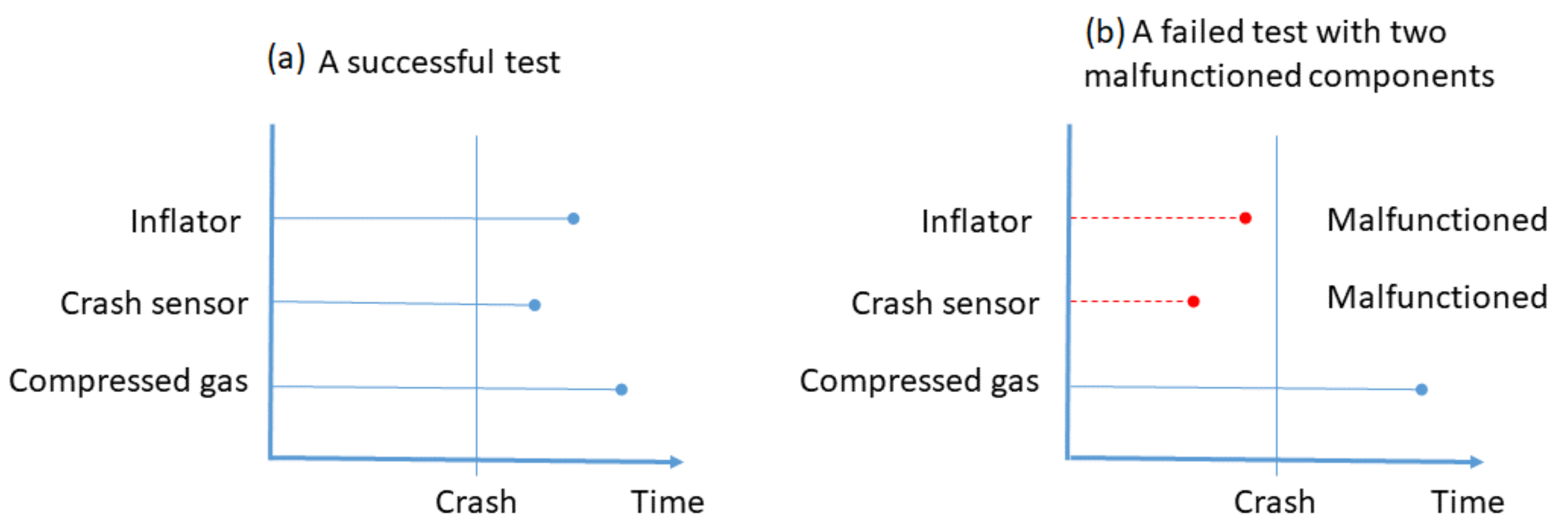
2. One-Shot Device Test Data with Multiple Failure Modes

Let us now consider one-shot devices with M components, Ω = { 1 , 2 , , M } , under a CSALT with I higher-than-normal stress conditions. For i = 1 , 2 , , I , K i devices are placed on test at stress level s i and tested at inspection time τ i . Let P ( Ω ) be the power set of Ω , representing the set of all possible combinations of failure modes (malfunctioned components). Note that the total number of possible combinations is P ( Ω ) = 2 M . Let n i , X denote the number of devices with the set of malfunctioned components X , so that X P ( Ω ) n i , X = K i . For instance, if there are M = 3 components, then Ω = { 1 , 2 , 3 } and P ( Ω ) = { , { 1 } , { 2 } , { 3 } , { 1 , 2 } , { 1 , 3 } , { 2 , 3 } , Ω } , where X = indicates that no malfunctioned components are present, while X = { 1 , 3 } , for example, indicates that components 1 and 3 have malfunctioned. Table 1 presents the form of one-shot device test data with M = 3 failure modes under a CSALT with I higher-than-normal stress conditions. For notational convenience, let us use z = { x i , τ i , n i , X , i = 1 , 2 , , I , X P ( Ω ) } to denote the observed data.

3. Exponential Lifetime Distributions with Gamma Frailty

Let T i , j , m denote the failure time of the m-th component of the j-th device in the i-th group, for i = 1 , 2 , , I , j = 1 , 2 , , K i , and m = 1 , 2 , , M . We now assume that, conditioned on a latent (unobserved) frailty γ i , j > 0 , T i , j , m follows an exponential distribution with rate parameter γ i , j λ i , m > 0 . The conditional cumulative distribution function (cdf) and probability density function (pdf) are then given by
F T i , j , m ( t | γ i , j ) = P ( T i , j , m t | γ i , j ) = 1 exp ( γ i , j λ i , m t ) ,
and
f T i , j , m ( t | γ i , j ) = γ i , j λ i , m exp ( γ i , j λ i , m t ) ,
for t > 0 . The corresponding conditional survival function is
R T i , j , m ( t | γ i , j ) = 1 F T i , j , m ( t | γ i , j ) = exp ( γ i , j λ i , m t ) , t > 0 .
We now assume that λ i , m = exp ( a m 0 + a m 1 s i ) links the failure rate of the m-th component with stress level s i . In the above formulation, the frailties γ ’s are assumed to be common among all the components within the same device but are different for different devices and follow a gamma distribution with scale parameter β > 0 and shape parameter 1 / β > 0 . The pdf of γ is then
f γ ( y ) = 1 Γ 1 β β 1 β y 1 β 1 exp y β , y > 0 , β > 0 .
Note that, to make the model identifiable [24], the mean of the frailty is 1, and the variance is β . Later on, some constraints on β will get imposed based on the mean and variance of the lifetimes of components.
For a device in the i-th test group, conditioned on γ , the failure times of those M components are independent, with the joint survival function of ( T i , 1 , T i , 2 , , T i , M ) given by
R T i , 1 , T i , 2 , , T i , M ( t 1 , t 2 , , t M ) = P m Ω { T i , m > t m } = 0 R T i , 1 ( t 1 | y ) R T i , 2 ( t 2 | y ) R T i , M ( t M | y ) f γ ( y ) d y = 1 + β m = 1 M λ i , m t m 1 β .
As the conditional survival function is R T i , m ( t | γ i , j ) = exp ( λ i , m t ) γ i , j , we may interpret that the frailty γ represents a random proportionality factor by which the hazard functions of the failure times of the components get modified and describes latent heterogeneity across devices as well as dependence between M components within each device arising from common environment/operation.
The joint (unconditional) pdf of ( T i , 1 , T i , 2 , , T i , M ) is readily obtained from (1) to be
f T i , 1 , T i , 2 , , T i , M ( t 1 , t 2 , , t M ) = M F T i , 1 , T i , 2 , , T i , M ( t 1 , t 2 , , t M ) t 1 t 2 t M = ( 1 ) M M R T i , 1 , T i , 2 , , T i , M ( t 1 , t 2 , , t M ) t 1 t 2 t M = m = 1 M λ i , m m = 1 M 1 ( 1 + m β ) 1 + β m = 1 M λ i , m t m 1 β + M .
In addition, from (1), we readily find
F T i , m ( t ) = P ( T i , m t ) = P ( T i , 1 > 0 , , T i , m t , , T i , M > 0 ) = 1 1 + β λ i , m t 1 β , t > 0 ,
which is a Lomax (or Pareto Type II) distribution with scale parameter ( β λ i , m ) 1 and shape parameter 1 / β (see [26,27]). Its mean and variance are, respectively, given by
μ T i , m = 1 λ i , m 1 β , ( β < 1 ) ,     and   σ T i , m 2 = 1 λ i , m 2 1 β 2 1 2 β , β < 1 2 .
Thus, there are constraints on β based on the assumption of existence of mean and variance. Next, we observe that, when β 0 ,   P m Ω { T i , m > t m } m = 1 M P ( T i , m > t m ) , indicating that the failure times of the components are dependent. Finally, the joint survival function in (1) can be rewritten in the form
P m Ω { T i , m > t m } = m = 1 M ( R T i , m ( t m ) ) β M + 1 1 β ,
which is the so-called Clayton survival copula. Its Kendall’s tau is τ = β / ( β + 2 ) , which indicates that a large value of β means stronger dependence between the components. Many studies have shown this connection between the gamma frailty model and the Clayton survival copula (see [24,28]). It is of interest to note here that the mean lifetime of the component, μ T i , m , is increasing with β , revealing that strong dependence between the components results in a larger mean lifetime of the component.
On the other hand, when β tends to zero, we have
F T i , m ( t ) = P ( T i , m t ) = 1 exp λ i , m t
and
R T i , 1 , T i , 2 , , T i , M ( t 1 , t 2 , , t M ) = exp m = 1 M λ i , m t m = m = 1 M R T i , m ( t m ) ,
where R T i , m ( t ) = 1 F T i , m ( t ) is the reliability function of T i , m , which corresponds to the case when the M components are independent. It also indicates that when β tends to zero, the variance of the frailty tends to zero, so that the frailties of all devices are simply equal to one. Consequently, the failure times of the components become independent.
Suppose X is the set of malfunctioned components in a device. Then, let X c denote the complement of X , representing the set of functioning components in the device, with X X c = Ω , X X c = , and | X | denoting the number of malfunctioned components in the device. Let us further define
g i ( X , t ) = P m X { T i , m > t } = 1 + β m X λ i , m t 1 β , and g i ( , t ) = 1 .
Then, by inclusion–exclusion principle, the probability of observing X at time t is given by
P i ( X , t ) = P m X { T i , m t } , k X c { T i , k > t } = 0 m X F T i , m ( t ) k X c R T i , k ( t ) f γ ( y ) d y = Y P ( X ) ( 1 ) | Y | g i ( { Y , X c } , t ) .
If we consider a device with M components, of which k components have malfunctioned, let us use X k for the set of any k malfunctioned components found in the device, and W = { Y , X c } . As | X c | = M k , we can see that | W | ranges from M k to M . Suppose | W | = n , where M k n M , with the corresponding | Y | = n M + k . Then, there are n n M + k = n M k repetitions of W for the device with k malfunctioned components. Hence, the probability that k malfunctioned components are found in the device is
P i ( X k , t ) = { W X k } Y P ( W ) ( 1 ) | Y | g i ( { Y , W c } , t ) = n = M k M ( 1 ) n M + k n M k X X n g i ( X , t ) .
Kuo et al. [9] defined a k-out-of-n system as a system of n components that functions if and only if at least k of the components work. Therefore, for a k-out-of-M structured device in the i-th group, the reliability of the device at time t is given by
R i , k ( t ) = d = 0 M k P i ( X d , t ) = n = k M d = 0 n k ( 1 ) d n d X X n g i ( X , t ) .
An illustration of this expression for a device with 2-out-of-4 structure is presented in Appendix A. Furthermore, the mean lifetime of such a device at stress level s i is given by
μ i , k = 0 R i , k ( t ) d t = n = k M d = 0 n k ( 1 ) d n d X X n ( 1 β ) m X λ i , m 1 = 1 1 β n = k M d = 0 n k ( 1 ) d n d X X n m X λ i , m 1 .
It is worth noting that the mean lifetime increases when the dependence ( β ) between the components in the device increases. Besides, this is a general expression of the mean lifetime for devices with components that are non-identical and dependent under the Clayton survival copula with Lomax distribution.

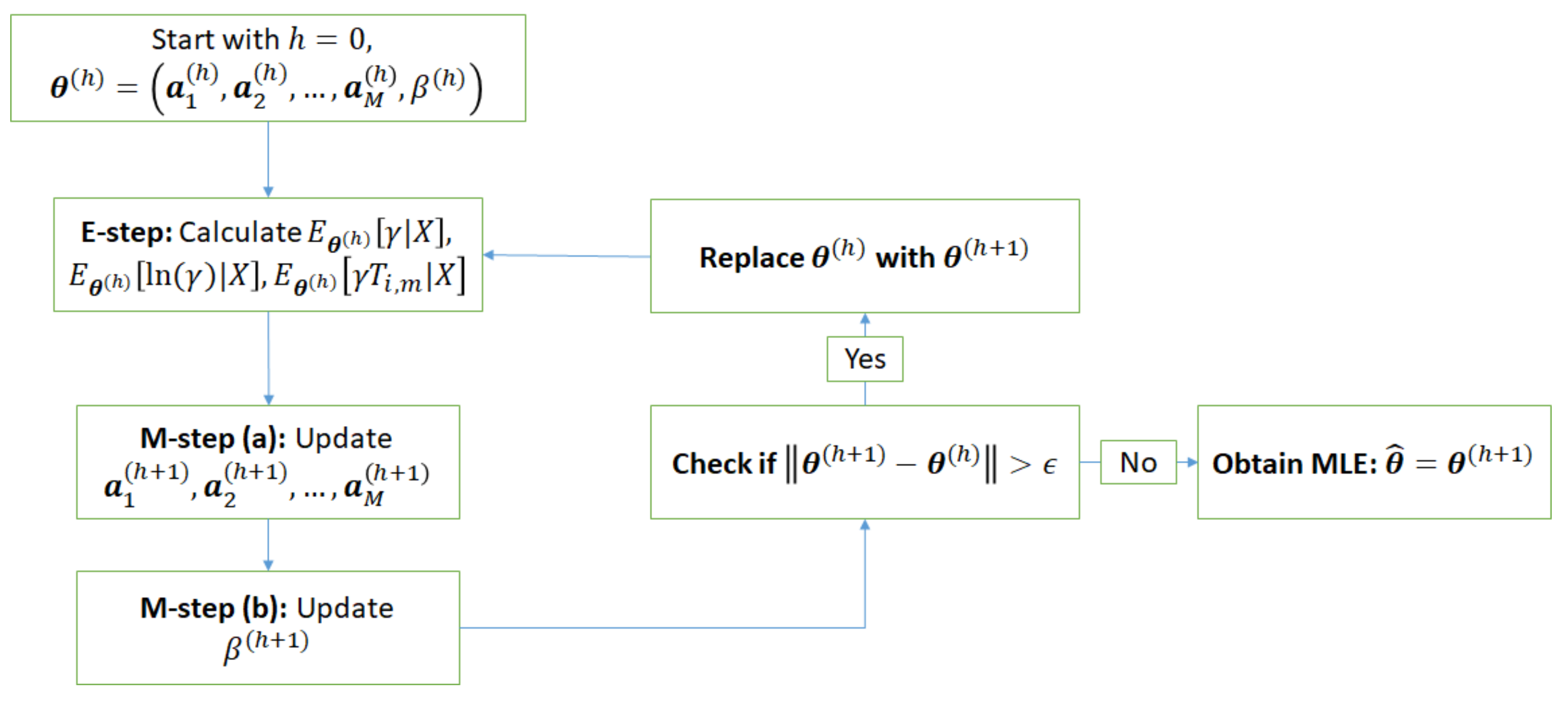
4. EM Algorithm for MLEs

For a one-shot device with M components, let a m = ( a m 0 , a m 1 ) be the vector of model parameters for the rate parameter of the exponential distribution for the m-th failure mode and β be the model parameter for the frailty term. Then, θ = ( a 1 , a 2 , , a M , β ) represents the vector of 2 M + 1 model parameters. It should be mentioned that a large number of components in the device would result in a high-dimensional vector of model parameters to be estimated, which may pose problems in finding accurate MLEs of model parameters. As a result, the estimators of some lifetime characteristics, for example, mean lifetime and reliability, may also face loss of precision. The observed log-likelihood function based on z = { x i , τ i , n i , X , i = 1 , 2 , , I , X P ( Ω ) } is then given by
( θ ) = i = 1 I X P ( Ω ) n i , X ln ( P i ( X , τ i ) ) + constant .
The EM algorithm [29] uses the observed data to iteratively compute the conditional expectation of the complete log-likelihood to provide imputed values (E-step) and then maximizes the conditional expectation of the complete log-likelihood to obtain updates of estimates (M-step). These two steps continue until convergence is reached to the desired level of accuracy. This technique is quite useful for finding the MLEs in the presence of missing data. We, therefore, utilize this technique to develop here an efficient EM algorithm for finding the MLEs from (5). For one-shot device test data, in a conventional EM algorithm, only the failure times of components are treated as missing data. The corresponding complete log-likelihood, with the joint (unconditional) densities, is
u n c i = 1 I j = 1 K i ln ( f T i , 1 , T i , 2 , , T i , M ( t i , j , 1 , t i , j , 2 , , t i , j , M ) ) + constant = i = 1 I j = 1 K i m = 1 M ln ( λ i , m ) + m = 1 M 1 ln ( 1 + m β ) 1 β + M ln 1 + β m = 1 M λ i , m t i , j , m + constant .
In the M-step, given the current estimate θ ( h ) , we update to get the estimate θ ( h + 1 ) by maximizing the conditional expectation of the complete log-likelihood, for which the first-order derivatives of the conditional expectation with respect to the model parameters are set to zero. The required first-order derivatives are
E θ ( h ) [ u n c ( θ ) | z ] a m 0 = i = 1 I K i 1 λ i , m 1 + M β E θ ( h ) T i , m 1 + β m = 1 M λ i , m T i , m z ,
E θ ( h ) [ u n c ( θ ) | z ] a m 1 = i = 1 I K i s i 1 λ i , m 1 + M β E θ ( h ) T i , m 1 + β m = 1 M λ i , m T i , m z ,
for m = 1 , 2 , , M , and
E θ ( h ) [ u n c ( θ ) | z ] β = i = 1 I K i m = 1 M 1 m 1 + m β + i = 1 I K i β 2 E θ ( h ) ln 1 + β m = 1 M λ i , m T i , m z i = 1 I K i 1 β + M E θ ( h ) m = 1 M λ i , m T i , m 1 + β m = 1 M λ i , m T i , m z .
These need three conditional expectations, which involve multiple integrals. We therefore partition the set of components in a device into three sets, namely, the set of the m-th component itself, { m } , the set of malfunctioned components at time τ i (excluding { m } ), X m , and the set of functioning components at time τ i (excluding { m } ), X m c . Then, we perform integration with respect to the lifetimes corresponding to X m , then followed by X m c , and finally with respect to { m } . In this manner, these conditional expectations are obtained. Now, let w i ( X ) = 1 + β m X λ i , m τ i , where X is the set of malfunctioned components in a device in the i-th test group. If m X ,
E θ ( h ) T i , m 1 + β m = 1 M λ i , m T i , m z = Y P ( X / { m } ) ( 1 ) | Y | w i ( { X c , Y } ) w i ( { X c , Y } ) 1 + 1 β w i ( { X c , Y , m } ) + λ i , m τ i w i ( { X c , Y , m } ) 1 + 1 β P i ( X , τ i ) λ i , m ( M β + 1 ) .
Conversely, if m X c ,
E θ ( h ) T i , m 1 + β m = 1 M λ i , m T i , m z = Y P ( X ) ( 1 ) | Y | w i ( { X c , Y } ) + λ i , m τ i w i ( { X c , Y } ) 1 + 1 β P i ( X , τ i ) λ i , m ( M β + 1 ) .
In addition,
E θ ( h ) m = 1 M λ i , m T i , m 1 + β m = 1 M λ i , m T i , m z = 1 β 1 Y P ( X ) ( 1 ) | Y | w i ( { X c , Y } ) 1 + 1 β P i ( X , τ i ) ( M β + 1 ) ,
and
E θ ( h ) ln 1 + β m = 1 M λ i , m T i , m z = 1 P i ( X , τ i ) Y P ( X ) ( 1 ) | Y | w i ( { X c , Y } ) ln ( w i ( { X c , Y } ) ) + m = 1 M M m + 1 β 1 .
In a more general EM framework, the failure time for each component in the device as well as the frailty for each device could be treated as latent variables. Then, by assuming first that they are observed, the complete log-likelihood is given by
c = i = 1 I j = 1 K i m = 1 M ln ( f T i , m ( t i , j , m | γ i , j ) ) + ln ( f γ ( γ i , j ) ) + constant = i = 1 I j = 1 K i m = 1 M ln ( λ i , m ) γ i , j m = 1 M λ i , m t i , j , m + M + 1 β 1 ln ( γ i , j ) γ i , j β i = 1 I K i ln Γ 1 β + 1 β ln ( β ) + constant .
In the M-step, the first-order derivatives of the conditional expectation, E θ ( h ) [ c ( θ ) | z ] , with respect to the model parameters are obtained as follows:
E θ ( h ) [ c ( θ ) | z ] a m 0 = i = 1 I K i 1 λ i , m E θ ( h ) [ γ T i , m | z ] ,
E θ ( h ) [ c ( θ ) | z ] a m 1 = i = 1 I K i s i 1 λ i , m E θ ( h ) [ γ T i , m | z ] ,
for m = 1 , 2 , , M , and
E θ ( h ) [ c ( θ ) | z ] β = i = 1 I K i β 2 E θ ( h ) [ γ | z ] E θ ( h ) [ ln ( γ ) | z ] + ln ( β ) + Ψ 1 β 1 ,
where Ψ ( · ) is the digamma function.
In this setup, although there is no closed-form solution for this maximization problem, we can separately update a 1 ( h + 1 ) , a 2 ( h + 1 ) , , a M ( h + 1 ) and β ( h + 1 ) , instead of updating these 2 M + 1 model parameters simultaneously. The maximization problem for the original vector of 2 M + 1 model parameters in the M-step simplifies to M + 1 sub-maximization problems for a vector of at most two model parameters, which makes the M-step more efficient and stable during the updating process.
This approach also requires three conditional expectations in the E-step, namely, E θ ( h ) [ γ | z ] , E θ ( h ) [ ln ( γ ) | z ] and E θ ( h ) [ γ T i , m | z ] , which are simple and have explicit forms. First, we have
0 γ exp ( ϕ γ ) f γ ( γ ) d γ = 0 1 Γ 1 β β 1 β γ 1 β exp γ 1 β + ϕ d γ = 1 + β ϕ 1 β + 1
and
0 ln ( γ ) exp ( ϕ γ ) f γ ( γ ) d γ = 1 + β ϕ 1 β Ψ 1 β ln 1 β + ϕ .
Suppose X is the set of malfunctioned components in a device in the i-th group. Let us now define
g i , u ( X ) = ( w i ( X ) ) 1 β + u = 1 + β m X λ i , m τ i 1 β + u
and
h i ( X ) = Ψ 1 β ln 1 β + τ i m X λ i , m .
Thence, we obtain
E θ ( h ) [ γ | X ] = 0 γ k X F T i , k ( τ i | γ ) l X c R T i , l ( τ i | γ ) f γ ( γ ) d γ P i ( X , τ i ) = 0 k X F T i , k ( τ i | γ ) l X c R T i , l ( τ i | γ ) 1 Γ 1 β β 1 β γ 1 β exp γ β d γ P i ( X , τ i ) = Y P ( X ) ( 1 ) | Y | g i , 1 ( { Y , X c } ) Y P ( X ) ( 1 ) | Y | g i , 0 ( { Y , X c } ) ,
E θ ( h ) [ ln ( γ ) | X ] = Y P ( X ) ( 1 ) | Y | g i , 0 ( { Y , X c } ) h i ( { Y , X c } ) Y P ( X ) ( 1 ) | Y | g i , 0 ( { Y , X c } ) .
Now, there are two cases for E θ ( h ) [ γ T i , m | X ] . If m X c ,
E θ ( h ) [ γ T i , m | X ] = 0 τ i γ t m f T i , m ( t m | γ ) d t m k X F T i , k ( τ i | γ ) l X c / { m } R T i , l ( τ i | γ ) f γ ( γ ) d γ P i ( X , τ i ) = 1 λ i , m + τ i E θ ( h ) [ γ | X ] .
On the other hand, if m X ,
E θ ( h ) [ γ T i , m | X ] = 0 0 τ i γ t m f T i , m ( t m | γ ) d t m k X / { m } F T i , k ( τ i | γ ) l X c R T i , l ( τ i | γ ) f γ ( γ ) d γ P i ( X , τ i ) = 1 λ i , m τ i E θ ( h ) [ γ | X / { m } ] P i ( X / { m } , τ i ) P i ( X , τ i ) .
Now, a general EM algorithm in this setup can be stated as follows.
Suppose θ ( h ) = ( a 1 ( h ) , a 2 ( h ) , , a M ( h ) , β ( h ) ) is given in the h-th step of iteration. Then:
S1:
In the E-step, find the three conditional expectations from (12)–(15);
S2:
In the M-step, using the above conditional expectations and optimization tools:
(a)
Update the estimate a m ( h + 1 ) from (9) and (10), for m = 1 , 2 , , M ;
(b)
Set β ( h + 1 ) = 0.5 exp ( exp ( b ) ) and update the estimate β ( h + 1 ) from (11) by solving for b such that β ( h + 1 ) is bounded between 0 and 0.5;
S3:
Repeat S1 and S2 until convergence is reached to the desired level of accuracy, with the current θ ( h + 1 ) as the MLE of the model parameter, denoted by θ ^ .
The flowchart of EM algorithm is presented in Figure 2.

5. Interval Estimation

In the preceding section, we have presented a general EM algorithm for finding the MLE of model parameter, θ ^ . Here, we present the asymptotic confidence intervals for model parameter, θ , which will be useful for making inference about the model parameter based on one-shot device test data, when the sample size is sufficiently large. The asymptotic confidence intervals need the asymptotic variance-covariance matrix of the MLE of model parameter, V ( θ ^ ) , which is given by the inverse of the observed information matrix of the MLE, I ( θ ^ ) . Under the EM framework, the observed information matrix can be obtained by using the missing information principle [30]. In one-shot device test data, wherein all the lifetimes are censored, the observed information matrix is
I ( θ ^ ) = E 2 ( θ ) θ θ θ = θ ^ = i = 1 I X P ( Ω ) K i P i ( X , τ i ; θ ^ ) P i ( X , τ i ; θ ^ ) θ P i ( X , τ i ; θ ^ ) θ ,
where
P i ( X , τ i ; θ ^ ) a m 0 = τ i λ ^ i , m Y P ( X ) ( 1 ) | Y | + 1 I m { Y , X c } 1 + β ^ k { Y , X c } λ ^ i , k τ i 1 β ^ 1 , P i ( X , τ i ; θ ^ ) a m 1 = τ i λ ^ i , m s i Y P ( X ) ( 1 ) | Y | + 1 I m { Y , X c } 1 + β ^ k { Y , X c } λ ^ i , k τ i 1 β ^ 1 , P i ( X , τ i ; θ ^ ) β = Y P ( X ) ( 1 ) | Y | β ^ 2 1 + β ^ m { Y , X c } λ ^ i , m τ i 1 β ^ × ln 1 + β ^ m { Y , X c } λ ^ i , m τ i β ^ τ i m { Y , X c } λ ^ i , m 1 + β ^ m { Y , X c } λ ^ i , m ,
with I m { Y , X c } denoting an indicator function that takes the value 1 if m { Y , X c } and takes the value 0 if m { Y , X c } . The derivation of the first-order derivatives is presented in detail in Appendix B. Thence, the 100 ( 1 δ ) % asymptotic confidence interval (ACI) for the model parameter θ is given by
θ ^ z 1 δ / 2 s e ( θ ) , θ ^ + z 1 δ / 2 s e ( θ ) ,
where s e ( θ ) is the standard error of the MLE, θ ^ , which is the corresponding diagonal entry of V ( θ ^ ) , and z 1 δ / 2 is the upper δ / 2 -th quantile of the standard normal distribution. It is worth noting that β is always in the interval from 0 to 0.5 for the finite mean and variance. Therefore, the confidence interval should be bounded within this interval.
Apart from the model parameter θ = ( a 10 , a 11 , , a M 0 , a M 1 , β ) , asymptotic confidence intervals for the system mean lifetime at normal operating condition s 0 are more useful for engineers and reliability practitioners in practice. First, we compute the first-order derivatives of the mean lifetime of a k-out-of-M system at s 0 ( μ 0 , k ) with respect to the model parameters ( a 10 , a 11 , , a M 0 , a M 1 , β ) , which are given by
μ 0 , k a m 0 = λ 0 , m 1 β n = k M d = 0 n k ( 1 ) d n d X X n , m r X λ 0 , r 2 , μ 0 , k a m 1 = λ 0 , m s 0 1 β n = k M d = 0 n k ( 1 ) d n d X X n , m r X λ 0 , r 2 , μ 0 , k β = 1 ( 1 β ) 2 n = k M d = 0 n k ( 1 ) d n d X X n r X λ 0 , r 1 ,
where λ 0 , m = exp ( a m 0 + a m 1 s 0 ) and X n , m is the set of any n malfunctioned components (including the m-th component) found in the device, for m = 1 , 2 , , M . We can then obtain the standard error of the system mean lifetime by using delta method [31], which is given by s e ( μ ) = P μ V ( θ ^ ) P μ T , where P μ = μ 0 , k a 10 , μ 0 , k a 11 , , μ 0 , k a M 0 , μ 0 , k a M 1 , μ 0 , k β is the vector of the first-order derivatives of the system mean lifetime. Thence, the 100 ( 1 δ ) % asymptotic confidence interval for the mean lifetime μ 0 , k is given by
μ ^ 0 , k z 1 δ / 2 s e ( μ ) , μ ^ 0 , k + z 1 δ / 2 s e ( μ ) .
It is worth noting that the system mean lifetime is non-negative. The lower bound of the interval may be truncated as 0. On the other hand, Balakrishnan and Ling [31] observed that the distribution of the MLE of mean lifetime is usually skewed when the sample size is small, and a log-transformation was suggested for constructing confidence intervals for the mean lifetime to ensure positive lower bound. The 100 ( 1 δ ) % transformed confidence interval (TCI) for the mean lifetime μ 0 , k is then given by
μ ^ 0 , k exp z 1 δ / 2 s e ( μ ) μ ^ 0 , k , μ ^ 0 , k exp z 1 δ / 2 s e ( μ ) μ ^ 0 , k .

6. Simulation Study

In this section, we perform a Monte Carlo simulation study first to verify the formula for the mean lifetime of a k-out-of-M structured device. Next, the performance of the developed inferential methods for different degrees of dependence and different sample sizes is evaluated, in terms of bias, root mean square error (RMSE), and coverage probability (CP) and average width (AW) of 95% ACI and TCI. Finally, a power analysis is carried out for comparing the performance of the ACI method and the likelihood ratio test (LRT) for testing the hypothesis of independence of components within devices.
Here, we present two simulation methods for generating component lifetimes under Clayton survival copula with Lomax distributions and consider one-shot devices with M = 4 components. The lifetimes of the components are assumed to follow Clayton survival copula with Lomax distributions with the joint survival function in (3). We set ( a 10 , a 11 ) = ( 6 , 0.05 ) , ( a 20 , a 21 ) = ( 6.5 , 0.06 ) , ( a 30 , a 31 ) = ( 7 , 0.07 ) , ( a 40 , a 41 ) = ( 8 , 0.08 ) , and s 0 = 25 , so that the corresponding failure rates are ( λ 1 , λ 2 , λ 3 , λ 4 ) = ( 0.0086 , 0.00673 , 0.0052 , 0.0024 ) . In addition, β { 0.1 , 0.3 , 0.4 } is taken to represent different degrees of dependence between the components in the device.

6.1. Simulation by Using Copula

We consider the conditional sampling method [32,33] to generate the lifetimes of the components for 100 , 000 devices. For this purpose, we assume that ( U 1 , U 2 , U 3 , U 4 ) have the joint survival Clayton survival copula of the form
C ¯ ( u 1 , u 2 , u 3 , u 4 ) = P ( U 1 > u 1 , U 2 > u 2 , U 3 > u 3 , U 4 > u 4 ) = ( u 1 β + u 2 β + u 3 β + u 4 β 3 ) 1 β .
It then follows that the conditional survival function of U 2 , given U 1 = u 1 , is
v 2 = P ( U 2 > u 2 | U 1 = u 1 ) = C ¯ ( u 1 , u 2 , 1 , 1 ) u 1 = { 1 u 1 β ( 1 u 2 ) β } 1 β + 1 β .
Similarly, for m = 3 and 4, we find
v m = P ( U m > u m | U 1 = u 1 , U 2 = u 2 , , U m 1 = u m 1 ) = m 1 C ¯ ( u 1 , u 2 , , u m , 1 , , 1 ) u 1 u 2 u m 1 m 1 C ¯ ( u 1 , u 2 , , u m 1 , 1 , , 1 ) u 1 u 2 u m 1 = u 1 β + u 2 β + + u m β m + 1 u 1 β + u 2 β + + u m 1 β m + 2 1 + ( m 1 ) β β .
Then, the algorithm for the generation of lifetimes of the components is as follows:
S1:
Generate u 1 , v 2 , v 3 , and v 4 from the standard uniform distribution U ( 0 , 1 ) ;
S2:
From (16), compute u 2 = 1 ( 1 v 2 ) β β + 1 u 1 β 1 β ;
S3:
From (17), for m = 3 and 4, compute
u m = v m β ( m 1 ) β + 1 1 j = 1 m 1 u j β ( m 2 ) v m β ( m 1 ) β + 1 + ( m 1 ) 1 β ;
S4:
Finally, from (2), for m = 1 , 2 , 3 , and 4, compute t m = u m β 1 β λ m .

6.2. Simulation by Using Frailty

In addition, the simulation can be done in another way by using frailty. We first consider the common frailty from the gamma distribution. When the frailty is given, we then use the conditional independence to simulate the component lifetimes, as the conditional survival function is R T i , m ( t | γ i , j ) = exp ( λ i , m t ) γ i , j = exp λ i , m γ i , j t , for m = 1 , 2 , , M , and the component lifetimes are conditionally independent. The algorithm of the generation of lifetimes of the components then is as follows:
S1:
Generate the frailty γ from the gamma distribution with scale parameter β > 0 and shape parameter 1 / β > 0 ;
S2:
Generate u 1 , u 2 , u 3 , and u 4 from the standard uniform distribution U ( 0 , 1 ) ;
S3:
Finally, compute t m = ln ( 1 u m ) γ λ m .
For these two simulation methods, we arrange the lifetimes of the components in ascending order, denoted by t [ 1 ] t [ 2 ] t [ 3 ] t [ 4 ] . Then, the lifetime of the k-out-of-4 structured device is t [ 5 k ] , for k = 1 , 2 , 3 , 4 .
Table 2 shows the empirical mean lifetimes of the k-out-of-4 structured devices obtained from the simulation method by using frailty are quite close to the theoretical mean lifetimes computed from (4) for all degrees of dependence considered. This reveals that the formula in (4) is accurate for computing the mean lifetime of the k-out-of-M structured devices. More importantly, the simulation method by using frailty is more convenient, efficient, and accurate than using copula to generate dependent component lifetimes.
Next, we consider the same setting of model parameters and evaluate the performance of the developed inferential methods for various sample sizes K { 30 , 50 , 100 } . The setup of CSALTs with two inspection times and three stress levels for one-shot devices is as detailed in Table 3. The results obtained from the simulation study, based on 1,000 Monte Carlo simulations, are presented in Table 4, Table 5, Table 6, Table 7 and Table 8. The MLEs of model parameters based on the EM algorithm were obtained by terminating when | | θ ( h ) θ ( h + 1 ) | | < 1 × 10 5 . From Table 4, Table 5 and Table 6, we observe that the bias of the MLEs of model parameters are all small and that the RMSE decreases when the sample size gets larger. For the ACIs, the coverage probabilities maintain the nominal level of 95%, while the average width of the intervals becomes smaller when the sample size increases. Thus, all the proposed inferential methods perform quite satisfactorily.
Table 7 and Table 8 show that large sample sizes are required for (i) devices with parallel structure (small k) and (ii) components with high dependence (large β ); also, the inferential methods for the mean lifetime of the device at normal operating condition perform well in the case of low dependence (small β ) and the sample size being sufficiently large or in the case of components with moderate dependence but the device being in series structure (large k). If we wish to estimate the mean lifetime of devices in which components have moderate or even high dependence and are placed in parallel, a larger number of devices are needed for constant-stress accelerated life-testing. Table 8 further presents the performance of the 95% ACI and TCI for the mean lifetime of the device. We observe that the coverage probability is deflated (below 95%) when K 50 , β 0.3 and k 3 . Thus, we can conclude that the ACIs generally work well when the sample size is large, or the components are close to independent ( β is small), or the components are placed in parallel (k is small). Not surprisingly, the log-transformation provides an appealing adjustment on the confidence intervals, and the TCIs consequently maintain the nominal level of 95% for all considered cases.
From a practical viewpoint, it will be of great interest to test whether the component lifetimes in a device are independent. Suppose the level of significance δ is fixed. As the component lifetimes are not independent when β > 0 , it is reasonable to consider one-sided confidence interval. In this case, the decision is simply whether the lower bound of the confidence interval, that is β ^ z 1 δ s e ( β ) , is greater than zero or not. If the lower bound is greater than zero, we can conclude that the component lifetimes are not independent. Apart from this asymptotic confidence interval method, the LRT can also be used for testing this hypothesis of independence. The observed log-likelihood function for the frailty model with correlation based on data z is as presented in (5). As the independence model corresponds to the case β = 0 , the observed log-likelihood function for the independence model based on data z is given by
i n d ( θ ) = i = 1 I X P ( Ω ) n i , X m X ln F T i , m ( τ i ) .
Thence, the LRT statistic for testing independence based on the frailty model can be given as
Λ L R T = 2 ( i n d ( θ ^ i n d ) ( θ ^ ) ) ,
where θ ^ and θ ^ i n d are the MLEs of model parameter θ for the frailty and independence models, respectively. As β = 0 lies on the boundary of the parameter space and the difference in the numbers of unknown model parameters between the frailty and independence models is 1, according to [34], the asymptotic null distribution of the LRT statistic can be approximated by a mixture of chi-square distributions, that is, P ( Λ L R T λ ) = 0.5 + 0.5 P ( χ 1 2 λ ) , where χ 1 2 is the chi-square random variable with 1 degree of freedom. We can then conclude that the component lifetimes are not independent when P ( Λ L R T λ ^ ) > 1 δ , where λ ^ is calculated from (18) by using the MLEs of model parameters for the frailty and independence models. Table 9 presents the power comparison for testing the hypothesis of independence among the components in the device between the ACI and LRT methods for several sample sizes and various degrees of dependence, at δ = 0.05 level of significance, based on 1,000 Monte Carlo simulations. The results show that the LRT outperforms the ACI method for identifying the dependence between components when the component lifetimes are indeed dependent, but the LRT does possess a higher probability of type I error when the component lifetimes are indeed independent and the sample size is not sufficiently large.

7. Illustrative Examples

7.1. Class-H Failure Mode Data

Let us first consider the Class-H failure modes data [6], in the form of one-shot device test data with two failure modes (Turn [T] and Ground [G]). The original data includes the failure times (in hours) for the failure modes of motorettes tested at temperatures of 374, 428, 464, and 500° F. In actual use, each motorette may be inspected once at a pre-specified time, in which case the modified data do become a one-shot device test data with two failure modes, and the corresponding data are as presented in Table 10. Table 11 presents the MLEs of model parameters as well as the 95% ACIs. In addition, the mean lifetimes of devices with series and parallel structures at the normal operating condition s 0 = 356 ° F are estimated to be 2245 h and 39,885 h, respectively. On the other hand, under the independence model, the estimates of the corresponding mean lifetimes turn out to be 1122 h and 19,942 h. These do show that the independence assumption results in seriously underestimating the mean lifetimes at the normal operating condition. The Class H failure modes dataset contains two failure modes but the sample size is quite small, and the ACI for β further shows that the correlation between these two failure modes is not significant.

7.2. Mice Tumor Toxicological Data

We next consider ED01 data presented in [35]. These tumor toxicological data present the numbers of deaths and sacrifices with and without bladder tumors on 671 mice at each of three inspection times. Each of those mice was either in a control group or an experimental group with high dose level of the known carcinogen 2-AAF. We can treat the death ( D ) and the appearance of bladder tumors ( T ) as two failure modes, Ω = { D , T } , and the exact death time and the onset time of the tumor of each mouse are either right- or left-censored. Table 12 and Table 13 present the ED01 data and the connections between the outcomes and the censoring in the ED01 data, respectively. The MLEs of model parameters and the corresponding 90% and 95% ACIs are presented in Table 14. The 90% ACI for β reveals that a high dose of the chemical induces an early onset of bladder tumors. Besides, there is a positive correlation between the onset time of bladder tumor and the death time. We may therefore conclude that the chemical would not result in an early death, but it would induce an early onset of bladder tumors which would cause a high risk of death.

7.3. Simulated Data

To illustrate the EM algorithm for data with more than two failure modes, we now consider a simulated one-shot device test data with M = 4 failure modes presented in Table 15. The simulated data is generated with model parameters ( a 10 , a 11 ) = ( 6 , 0.05 ) , ( a 20 , a 21 ) = ( 6.5 , 0.06 ) , ( a 30 , a 31 ) = ( 7 , 0.07 ) , ( a 40 , a 41 ) = ( 8 , 0.08 ) , and β = 0.3 . A comparison of the MLEs obtained by the use of EM algorithm and by the general optimization tool, “optim()” in R, is first made. We chose the initial values of the model parameters to be ( a 10 ( 0 ) , a 11 ( 0 ) , a 20 ( 0 ) , a 21 ( 0 ) , a 30 ( 0 ) , a 31 ( 0 ) , a 40 ( 0 ) , a 41 ( 0 ) ) = ( 5.95 , 0.01 , 6.59 , 0.14 , 7.05 , 0.2 , 7.87 , 0.04 ) and considered β ( 0 ) { 0.2 , 0.3 , 0.4 } to evaluate the robustness of these two methods. Table 16 presents the values of MLEs and the computational times for various choices of β ( 0 ) as an initial value, which do reveal the EM algorithm to be quite robust and efficient timewise in determining the MLEs. In addition, we obtained β ^ = 0.5172 and 0.6046 by using “optim()” when β ( 0 ) was set to be 0.2 and 0.4, respectively. Clearly, these estimates are out of the range of [0, 0.5] for β . In addition, the 95% ACIs for the model parameters are presented in Table 17, which do show that the component lifetimes are not independent. Moreover, the estimates of the mean lifetimes of k-out-of-4 structured devices at the normal operating condition s 0 = 25 are 437.053, 213.861, 112.827, and 47.808 for k = 1 , 2 , 3 , 4 , respectively. Under the independence assumption, the estimates of the corresponding mean lifetimes turn out to be 325.329, 159.140, 83.972, and 35.586. Here again, we observe that the independence assumption for the components in the device results in severely underestimating the mean lifetimes at the normal operating condition.

8. Concluding Remarks

In this paper, we have developed an efficient EM algorithm that provides a stable and robust method for finding the MLEs of model parameters for a k-out-of-M structured one-shot device with dependent components having exponential lifetime distribution under gamma frailty to capture the dependence. This is indeed identical to the Clayton survival copula with Lomax lifetime distribution, based on one-shot device test data with multiple failure modes collected from a CSALT. The mean lifetime of k-out-of-M structured devices has also been derived explicitly. The extensive Monte Carlo simulation studies carried out show that the developed inferential methods all perform very well for various sample sizes and different degrees of dependence. The illustrative examples also demonstrate that the developed EM algorithm is less sensitive to the choice of initial values, compared to the common optimization tool, “optim” in R. The R codes that implement the proposed methodologies can be available from the first author upon request.
It is important to note that component lifetimes are often assumed to be independent and identical in reliability literature though often not realistic in many practical situations. However, this wrong assumption may result in a serious bias in the estimation of lifetime characteristics such as mean lifetime. In this study, the expression derived for the mean lifetime is a general result for devices with components that are non-identical and dependent due to the common gamma frailty. The illustrative examples show that, when the model with independence assumption is wrongly assumed for analyzing data when the components in the device are dependent, a significant bias results in the estimate of the mean lifetime of the device.
Furthermore, it will be of great interest to find similar connections between other frailty and copula models and to develop similar results for one-shot devices with more flexible lifetime distributions for components such as Weibull and gamma. In most cases, the failure rates of components are greater than their initial failure rates. The exponential distribution with a constant failure rate becomes very restrictive in practice. Both Weibull and gamma distributions can model components with increasing and decreasing failure rates and contain the exponential lifetime distribution as a special case. Thus, they are popular in reliability and survival studies. We can also consider the development of optimal designs for one-shot device in the considered scenario under some cost and efficiency constraints. In line with [36], an efficient CSALT plan is designed for one-shot devices by obtaining the inspection frequency, the number of inspections at each test group, and the number of devices allocated for testing in order to minimize the asymptotic variance of the MLE of a lifetime characteristic under budget and time constraints. Moreover, several frailty models can be considered to model the dependence between the components, namely generalized gamma frailty, positive stable frailty, and inverse Gaussian frailty. When many frailty models are available for capturing the dependence between components, it is natural to select the best model for a given dataset in a statistical investigation. We are currently working on these problems and hope to report the findings in a future paper.

Author Contributions

Conceptualization, M.-H.L. and N.B.; methodology, M.-H.L. and N.B.; software, M.-H.L., C.Y. and H.Y.S.; validation, M.-H.L.; writing—original draft preparation, M.-H.L.; writing—review and editing, M.-H.L. and N.B.; supervision, M.-H.L., N.B. and H.Y.S.; project administration, M.-H.L. and N.B.; funding acquisition, M.-H.L. and N.B. All authors have read and agreed to the published version of the manuscript.

Funding

This work of the first author was supported by the Dean’s Research Fund of the Faculty of Liberal Arts and Social Sciences, The Education University of Hong Kong, Hong Kong Special Administrative Region, China (Project No. FLASS/DRF 04618), while that of the second author was funded by the Natural Sciences and Engineering Research Council of Canada through an Individual Discovery Grant RGPIN-2020-06733.

Institutional Review Board Statement

Not applicable.

Informed Consent Statement

Not applicable.

Acknowledgments

Our sincere thanks go to the editor of this special issue for sending an invitation to us which provided an impetus for preparing this article. We also thank the referees for their constructive comments and suggestions.

Conflicts of Interest

The authors declare no conflict of interest. The funders had no role in the design of the study; in the collection, analyses, or interpretation of data; in the writing of the manuscript, or in the decision to publish the results.

Abbreviations

The following abbreviations are used in this manuscript:
ALTsAccelerated life-tests
EMExpectation–maximization
MLEsMaximum likelihood estimates
CSALTConstant-stress accelerated life-test
cdfCumulative distribution function
pdfProbability density function
E-stepExpectation step
M-stepMaximization step
ACIAsymptotic confidence interval
TCITransformed confidence interval
RMSERoot mean square error
CPCoverage probability
AWAverage width
LRTLikelihood ratio test

Appendix A

Suppose a device consists of M = 4 components and the set of malfunctioned components is X = { 1 , 2 } . Then, X c = { 3 , 4 } and P ( X ) = { , { 1 } , { 2 } , { 1 , 2 } } . The probability of observing X at time t is
P i ( X , t ) = P ( T i , 1 t , T i , 2 t , T i , 3 > t , T i , 4 > t ) = P ( T i , 3 > t , T i , 4 > t ) P ( ( T i , 1 t , T i , 2 t ) c , T i , 3 > t , T i , 4 > t ) = g i ( { 3 , 4 } , t ) [ g i ( { 1 , 3 , 4 } , t ) + g i ( { 2 , 3 , 4 } , t ) g i ( { 1 , 2 , 3 , 4 } , t ) ] = g i ( { 3 , 4 } , t ) g i ( { 1 , 3 , 4 } , t ) g i ( { 2 , 3 , 4 } , t ) + g i ( { 1 , 2 , 3 , 4 } , t ) = 1 + β ( λ i , 3 + λ i , 4 ) t 1 β 1 + β ( λ i , 1 + λ i , 3 + λ i , 4 ) t 1 β 1 + β ( λ i , 2 + λ i , 3 + λ i , 4 ) t 1 β + 1 + β ( λ i , 1 + λ i , 2 + λ i , 3 + λ i , 4 ) t 1 β .
The probability that k = 2 malfunctioned components are found in the device is
P i ( X 2 , t ) = g i ( { 3 , 4 } , t ) g i ( { 1 , 3 , 4 } , t ) g i ( { 2 , 3 , 4 } , t ) + g i ( { 1 , 2 , 3 , 4 } , t ) + g i ( { 2 , 4 } , t ) g i ( { 1 , 2 , 4 } , t ) g i ( { 2 , 3 , 4 } , t ) + g i ( { 1 , 2 , 3 , 4 } , t ) + g i ( { 1 , 4 } , t ) g i ( { 1 , 2 , 4 } , t ) g i ( { 1 , 3 , 4 } , t ) + g i ( { 1 , 2 , 3 , 4 } , t ) + g i ( { 2 , 3 } , t ) g i ( { 1 , 2 , 3 } , t ) g i ( { 2 , 3 , 4 } , t ) + g i ( { 1 , 2 , 3 , 4 } , t ) + g i ( { 1 , 3 } , t ) g i ( { 1 , 2 , 3 } , t ) g i ( { 1 , 3 , 4 } , t ) + g i ( { 1 , 2 , 3 , 4 } , t ) + g i ( { 1 , 2 } , t ) g i ( { 1 , 2 , 3 } , t ) g i ( { 1 , 2 , 4 } , t ) + g i ( { 1 , 2 , 3 , 4 } , t ) = 2 2 X X 2 g i ( X , t ) 3 2 X X 3 g i ( X , t ) + 4 2 X X 4 g i ( X , t ) .
Thence, the reliability of a 2-out-of-4 structured device in the i-th group at time t is
R i , 2 ( t ) = P i ( X 0 , t ) + P i ( X 1 , t ) + P i ( X 2 , t ) = 4 4 X X 4 g i ( X , t ) + 3 3 X X 3 g i ( X , t ) 3 2 X X 4 g i ( X , t ) + 2 2 X X 2 g i ( X , t ) 3 2 X X 3 g i ( X , t ) + 4 2 X X 4 g i ( X , t ) = 2 0 X X 2 g i ( X , t ) + 3 0 3 1 X X 3 g i ( X , t ) + 4 0 4 1 + 4 2 X X 4 g i ( X , t ) = X X 2 g i ( X , t ) 2 X X 3 g i ( X , t ) + 3 X X 4 g i ( X , t ) .

Appendix B

We have
P i ( X , τ i ; θ ) a m 0 = Y P ( X ) ( 1 ) | Y | g i ( { Y , X c } , τ i ) ) a m 0 = Y P ( X ) ( 1 ) | Y | 1 + β k { Y , X c } λ i , k τ i 1 β a m 0 = τ i λ i , m Y P ( X ) ( 1 ) | Y | + 1 I m { Y , X c } 1 + β k { Y , X c } λ i , k τ i 1 β 1 ,
where I m { Y , X c } is an indicator function that takes value 1 if m { Y , X c } and takes value 0 if m { Y , X c } . Hence,
P i ( X , τ i ; θ ^ ) a m 0 = τ i λ ^ i , m Y P ( X ) ( 1 ) | Y | + 1 I m { Y , X c } 1 + β ^ k { Y , X c } λ ^ i , k τ i 1 β ^ 1 .
Similarly,
P i ( X , τ i ; θ ^ ) a m 1 = τ i λ ^ i , m s i Y P ( X ) ( 1 ) | Y | + 1 I m { Y , X c } 1 + β ^ k { Y , X c } λ ^ i , k τ i 1 β ^ 1 , P i ( X , τ i ; θ ^ ) β = Y P ( X ) ( 1 ) | Y | β ^ 2 1 + β ^ m { Y , X c } λ ^ i , m τ i 1 β ^ × ln 1 + β ^ m { Y , X c } λ ^ i , m τ i β ^ τ i m { Y , X c } λ ^ i , m 1 + β ^ m { Y , X c } λ ^ i , m .

References

  1. Bain, L.J.; Engelhardt, M. Reliability test plans for one-shot devices based on repeated samples. J. Qual. Technol. 1991, 23, 304–311. [Google Scholar] [CrossRef]
  2. Olwell, D.H.; Sorell, A.A. Warranty calculations for missiles with only current-status data, using Bayesian methods. In Proceedings of the Annual Reliability and Maintainability Symposium, International Symposium on Product Quality and Integrity (Cat. No. 01CH37179), Philadelphia, PA, USA, 22–25 January 2001; pp. 133–138. [Google Scholar]
  3. Newby, M. Monitoring and maintenance of spares and one shot devices. Reliab. Eng. Syst. Saf. 2008, 93, 588–594. [Google Scholar] [CrossRef]
  4. Fan, T.H.; Balakrishnan, N.; Chang, C.C. The Bayesian approach for highly reliable electro-explosive devices using one-shot device testing. J. Stat. Comput. Simul. 2009, 79, 1143–1154. [Google Scholar] [CrossRef]
  5. Zheng, J.; Li, Y.; Wang, J.; Shiju, E.; Li, X. Accelerated thermal aging of grease-based magnetorheological fluids and their lifetime prediction. Mater. Res. Express 2018, 5, 085702. [Google Scholar] [CrossRef]
  6. Nelson, W.B. Accelerated Testing: Statistical Models, Test Plans, and Data Analysis; John Wiley & Sons: Hoboken, NJ, USA, 2009. [Google Scholar]
  7. Meeker, W.Q.; Escobar, L.A. Statistical Methods for Reliability Data; John Wiley & Sons: New York, NY, USA, 2014. [Google Scholar]
  8. Balakrishnan, N.; Ling, M.H.; So, H.Y. Accelerated Life Testing of One-Shot Devices: Data Collection and Analysis; John Wiley & Sons: Hoboken, NJ, USA, 2021. [Google Scholar]
  9. Kuo, W.; Zhang, W.; Zuo, M. A consecutive-k-out-of-n: G system: The mirror image of a consecutive-k-out-of-n: F system. IEEE Trans. Reliab. 1990, 39, 244–253. [Google Scholar] [CrossRef]
  10. Coit, D.W.; Chatwattanasiri, N.; Wattanapongsakorn, N.; Konak, A. Dynamic k-out-of-n system reliability with component partnership. Reliab. Eng. Syst. Saf. 2015, 138, 82–92. [Google Scholar] [CrossRef]
  11. Ling, X.; Wei, Y.; Si, S. Reliability optimization of k-out-of-n system with random selection of allocative components. Reliab. Eng. Syst. Saf. 2019, 186, 186–193. [Google Scholar] [CrossRef]
  12. Cheng, Y.; Elsayed, E.A. Reliability modeling and prediction of systems with mixture of units. IEEE Trans. Reliab. 2015, 65, 914–928. [Google Scholar] [CrossRef]
  13. Cheng, Y.; Elsayed, E.A. Optimal sequential ALT plans for systems with mixture of one-shot units. IEEE Trans. Reliab. 2017, 66, 997–1011. [Google Scholar] [CrossRef]
  14. Cheng, Y.; Elsayed, E.A. Reliability modeling of mixtures of one-shot units under thermal cyclic stresses. Reliab. Eng. Syst. Saf. 2017, 167, 58–66. [Google Scholar] [CrossRef]
  15. Cheng, Y.; Elsayed, E.A. Reliability modeling and optimization of operational use of one-shot units. Reliab. Eng. Syst. Saf. 2018, 176, 27–36. [Google Scholar] [CrossRef]
  16. Zhang, X.P.; Shang, J.Z.; Chen, X.; Zhang, C.H.; Wang, Y.S. Statistical inference of accelerated life testing with dependent competing failures based on copula theory. IEEE Trans. Reliab. 2014, 63, 764–780. [Google Scholar] [CrossRef]
  17. Cooke, R.; Paulsen, J. Concepts for measuring maintenance performance and methods for analysing competing failure modes. Reliab. Eng. Syst. Saf. 1997, 55, 135–141. [Google Scholar] [CrossRef]
  18. Bocchetti, D.; Giorgio, M.; Guida, M.; Pulcini, G. A competing risk model for the reliability of cylinder liners in marine diesel engines. Reliab. Eng. Syst. Saf. 2009, 94, 1299–1307. [Google Scholar] [CrossRef]
  19. Balakrishnan, N.; So, H.Y.; Ling, M.H. EM algorithm for one-shot device testing with competing risks under Weibull distribution. IEEE Trans. Reliab. 2016, 65, 973–991. [Google Scholar] [CrossRef]
  20. Kotz, S.; Balakrishnan, N.; Johnson, N.L. Continuous Multivariate Distributions, 2nd ed.; John Wiley & Sons: New York, NY, USA, 2000. [Google Scholar]
  21. Sklar, A. Fonctions de repartition an dimensions et leurs marges. Publ. Inst. Stat. Univ. Paris 1959, 8, 229–231. [Google Scholar]
  22. Peng, W.; Li, Y.F.; Yang, Y.J.; Zhu, S.P.; Huang, H.Z. Bivariate analysis of incomplete degradation observations based on inverse Gaussian processes and copulas. IEEE Trans. Reliab. 2016, 65, 624–639. [Google Scholar] [CrossRef]
  23. Ling, M.H.; Chan, P.S.; Ng, H.K.T.; Balakrishnan, N. Copula models for one-shot device testing data with correlated failure modes. Commun. Stat.-Theory Methods 2021, 50, 3875–3888. [Google Scholar] [CrossRef]
  24. Liu, X. Planning of accelerated life tests with dependent failure modes based on a gamma frailty model. Technometrics 2012, 54, 398–409. [Google Scholar] [CrossRef]
  25. Tseng, S.T.; Hsu, N.J.; Lin, Y.C. Joint modeling of laboratory and field data with application to warranty prediction for highly reliable products. IIE Trans. 2016, 48, 710–719. [Google Scholar] [CrossRef]
  26. Nayak, T.K. Multivariate Lomax distribution: Properties and usefulness in reliability theory. J. Appl. Probab. 1987, 24, 170–177. [Google Scholar] [CrossRef]
  27. Johnson, N.L.; Kotz, S.; Balakrishnan, N. Continuous Univariate Distributions, 2nd ed.; John Wiley & Sons: New York, NY, USA, 1994; Volume 1. [Google Scholar]
  28. Hanagal, D.D.; Pandey, A. Gamma shared frailty model based on reversed hazard rate. Commun. Stat.-Theory Methods 2016, 45, 2071–2088. [Google Scholar] [CrossRef]
  29. McLachlan, G.J.; Krishnan, T. The EM Algorithm and Extensions; John Wiley & Sons: Hoboken, NJ, USA, 2007. [Google Scholar]
  30. Louis, T.A. Finding the observed information matrix when using the EM algorithm. J. R. Stat. Soc. Ser. B 1982, 44, 226–233. [Google Scholar]
  31. Balakrishnan, N.; Ling, M.H. Gamma lifetimes and one-shot device testing analysis. Reliab. Eng. Syst. Saf. 2014, 126, 54–64. [Google Scholar] [CrossRef]
  32. Nelsen, R.B. An Introduction to Copulas; Springer: New York, NY, USA, 2007. [Google Scholar]
  33. Hofert, M.; Kojadinovic, I.; Mächler, M.; Yan, J. Elements of Copula Modeling with R; Springer: New York, NY, USA, 2019. [Google Scholar]
  34. Balakrishnan, N.; Pal, S. Lognormal lifetimes and likelihood-based inference for flexible cure rate models based on COM-Poisson family. Comput. Stat. Data Anal. 2013, 67, 41–67. [Google Scholar] [CrossRef]
  35. Lindsey, J.C.; Ryan, L.M. A three-state multiplicative model for rodent tumorigenicity experiments. J. R. Stat. Soc. Ser. C 1993, 42, 283–300. [Google Scholar] [CrossRef]
  36. Balakrishnan, N.; Ling, M.H. Best constant-stress accelerated life-test plans with multiple stress factors for one-shot device testing under a Weibull distribution. IEEE Trans. Reliab. 2014, 63, 944–952. [Google Scholar] [CrossRef]
Figure 1. Component lifetimes in an automobile airbag system under (a) a successful crash test and (b) a failed crash test with two malfunctioned components.
Mathematics 09 03032 g001
Figure 2. The flowchart of EM algorithm to obtain the MLE of the model parameter θ ^ with the desired level of accuracy ϵ .
Mathematics 09 03032 g002
Table 1. Form of one-shot device test data with M = 3 failure modes, Ω = { 1 , 2 , 3 } .
TestStr.Insp.Number of Devices with the Set of Malfunctioned Components
Grp.Lvl.Time { 1 } { 2 } { 3 } { 1 , 2 } { 1 , 3 } { 2 , 3 } Ω
1 s 1 τ 1 n 1 , n 1 , { 1 } n 1 , { 2 } n 1 , { 3 } n 1 , { 1 , 2 } n 1 , { 1 , 3 } n 1 , { 2 , 3 } n 1 , Ω
2 s 2 τ 2 n 2 , n 2 , { 1 } n 2 , { 2 } n 2 , { 3 } n 2 , { 1 , 2 } n 2 , { 1 , 3 } n 2 , { 2 , 3 } n 2 , Ω
I s I τ I n I , n I , { 1 } n I , { 2 } n I , { 3 } n I , { 1 , 2 } n I , { 1 , 3 } n I , { 2 , 3 } n I , Ω
Table 2. The empirical mean lifetimes of k-out-of-4 structured devices obtained from the simulation methods by using copula (C) and frailty (F) and the theoretical mean lifetimes computed from (4) for k { 1 , 2 , 3 , 4 } .
DependenceMean Lifetime k = 1 k = 2 k = 3 k = 4
β = 0.1 Empirical (C)555.3440232.2293116.549848.1355
Empirical (F)556.7529232.3021116.579048.1404
Theoretical556.9071231.8686116.482248.0669
β = 0.3 Empirical (C)711.6244297.2964149.403162.0487
Empirical (F)716.3950298.7292149.772461.9213
Theoretical716.0235298.1167149.762961.8003
β = 0.4 Empirical (C)829.6855345.3503173.296271.9890
Empirical (F)835.3608347.8029174.723472.1004
Theoretical835.3608347.8029174.723472.1004
Table 3. The setting of CSALTs with two inspection times and three stress levels for one-shot devices.
Test GroupStress LevelInspection TimeNumber of Test Devices
1 s 1 = 35 τ 1 = 10 K 1 = K
2 s 2 = 35 τ 2 = 20 K 2 = K
3 s 3 = 45 τ 3 = 10 K 3 = K
4 s 4 = 45 τ 4 = 20 K 4 = K
5 s 5 = 55 τ 5 = 10 K 5 = K
6 s 6 = 55 τ 6 = 20 K 6 = K
Table 4. Values of bias, root mean square error (RMSE) of the MLEs, and coverage probability (CP) and average width (AW) of 95% ACI for the model parameters for various sample sizes in the case of low dependence ( β = 0.1 ) .
a 10 a 11 a 20 a 21 a 30 a 31 a 40 a 41 β
KMeasure−60.05−6.50.06−70.07−80.080.1
30BIAS−0.0670.001−0.0630.001−0.0560.001−0.1640.0030.022
RMSE0.8850.0180.9180.0190.9660.0201.2420.0250.107
CP0.9440.9530.9510.9520.9580.9570.9540.9590.993
AW3.4360.0723.5700.0743.7150.0764.8340.0970.489
50BIAS−0.0120.000−0.0380.001−0.0830.002−0.0710.0010.009
RMSE0.6820.0140.7230.0150.7380.0150.9540.0190.083
CP0.9460.9470.9460.9470.9570.9610.9490.9480.989
AW2.6290.0552.7420.0572.8700.0593.6920.0740.372
100BIAS−0.0160.000−0.0330.0010.0010.000−0.0310.0000.005
RMSE0.4930.0100.4970.0100.5310.0110.6680.0130.059
CP0.9420.9420.9490.9440.9400.9420.9540.9550.987
AW1.8540.0391.9310.0402.0040.0412.5910.0520.261
Table 5. Values of bias, root mean square error (RMSE) of the MLEs, and coverage probability (CP) and average width (AW) of 95% ACI for the model parameters for various sample sizes in the case of moderate dependence ( β = 0.3 ) .
a 10 a 11 a 20 a 21 a 30 a 31 a 40 a 41 β
KMeasure−60.05−6.50.06−70.07−80.080.3
30BIAS−0.0520.001−0.1040.002−0.1020.002−0.0740.0010.011
RMSE0.9060.0190.9800.0201.0210.0211.2330.0250.155
CP0.9560.9580.9540.9480.9490.9500.9650.9610.944
AW3.5710.0753.7120.0773.8700.0804.9120.0990.617
50BIAS−0.0250.000−0.0180.000−0.0620.001−0.0960.0020.006
RMSE0.6940.0140.7390.0150.7790.0161.0050.0200.126
CP0.9600.9630.9550.9620.9480.9470.9450.9440.928
AW2.7490.0582.8530.0592.9750.0613.7960.0770.476
100BIAS−0.0130.000−0.0020.000−0.0370.001−0.0300.0000.002
RMSE0.5070.0110.5240.0110.5500.0110.6790.0140.084
CP0.9470.9440.9460.9510.9510.9540.9480.9460.946
AW1.9370.0412.0070.0422.0920.0432.6490.0540.334
Table 6. Values of bias, root mean square error (RMSE) of the MLEs, and coverage probability (CP) and average width (AW) of 95% ACI for the model parameters for various sample sizes in the case of high dependence ( β = 0.4 ) .
a 10 a 11 a 20 a 21 a 30 a 31 a 40 a 41 β
KMeasure−60.05−6.50.06−70.07−80.080.4
30BIAS−0.1500.003−0.0330.001−0.1060.002−0.1850.0030.000
RMSE0.9580.0200.9860.0211.0200.0211.3220.0270.176
CP0.9560.9500.9440.9490.9490.9560.9540.9530.930
AW3.6580.0773.7550.0783.9210.0815.0090.1010.676
50BIAS−0.0910.002−0.0470.001−0.0390.001−0.1030.0020.009
RMSE0.7300.0150.7430.0150.7360.0151.0050.0200.136
CP0.9530.9520.9510.9500.9600.9580.9560.9510.946
AW2.8210.0592.9110.0613.0210.0623.8330.0770.529
100BIAS−0.0070.000−0.0350.001−0.0330.001−0.0260.0000.004
RMSE0.4940.0100.5300.0110.5580.0120.6860.0140.095
CP0.9570.9590.9490.9450.9400.9420.9530.9510.956
AW1.9720.0412.0520.0432.1300.0442.6800.0540.371
Table 7. Values of bias and root mean square error (RMSE) of MLE of μ 0 , k at normal operating condition s 0 = 25 for various sample sizes and various degrees of dependence.
β = 0.1 β = 0.3
k = 1 k = 2 k = 3 k = 4 k = 1 k = 2 k = 3 k = 4
K μ 0 , k 55623111648.0771629814961.80
30BIAS24637.549.411.7628852.2314.903.98
RMSE63494.3337.9614.72154445118353.64
50BIAS12621.875.380.7920939.5012.153.18
RMSE31968.9329.7511.7254715271.1827.81
100BIAS57.059.362.130.2381.7316.074.541.00
RMSE18041.5718.777.6126067.3831.4312.68
β = 0.4
k = 1 k = 2 k = 3 k = 4
K μ 0 , k 83534717472.10
30BIAS53010736.2010.83
RMSE43661058500201
50BIAS29765.5424.648.19
RMSE89624011345.50
100BIAS11025.748.922.64
RMSE33298.2546.9019.05
Table 8. Values of coverage probability (CP) and average width (AW) of 95% ACI and TCI for μ 0 , k at normal operating condition s 0 = 25 for various sample sizes and various degrees of dependence.
ACITCI
k = 1 k = 2 k = 3 k = 4 k = 1 k = 2 k = 3 k = 4
β = 0.1 μ 0 , k 55623111648.0755623111648.07
30CP0.9690.9770.9590.9430.9800.9660.9670.958
AW190334914859.15266437615862.90
50CP0.9520.960.9460.9410.9620.9610.9610.955
AW103823710743.64116924711145.14
100CP0.9670.9690.9620.9500.9630.9600.9610.954
AW61715673.2730.1164715974.4430.60
β = 0.3 μ 0 , k 71629814961.8071629814961.80
30CP0.9540.9440.9160.9020.9810.9680.9560.940
AW233955724296.093053624268106
50CP0.9410.9410.920.9070.9600.9600.9520.942
AW145437917370.08166440218374.03
100CP0.9570.9570.9470.9480.9600.9650.9510.951
AW90524911848.5495825612149.79
β = 0.4 μ 0 , k 83534717472.1083534717472.10
30CP0.9540.9490.9310.9080.9720.9660.9630.954
AW31246893011184335785339133
50CP0.9430.9420.9230.9060.9650.9660.9540.955
AW182248522390.08212852323996.51
100CP0.9380.9420.9240.9220.9640.9640.9570.950
AW108432315463.15115533515965.28
Table 9. Power of detection of dependence by using ACI and LRT for various sample sizes and various degrees of dependence, at δ = 0.05 level of significance.
LRTACI
K β = 0 β = 0 . 1 β = 0 . 3 β = 0 . 4 β = 0 β = 0 . 1 β = 0 . 3 β = 0 . 4
300.2590.4190.8360.9090.0300.1610.6610.805
500.1000.3430.9180.9860.0310.2250.8620.969
1000.0610.4910.9961.0000.0390.4330.9911.000
Table 10. Modified Class-H failure modes data [6], with Ω = { T , G } .
i s i τ i n n { T } n { G } n Ω
137480000104
237410,0001400
342825001202
442830002003
546416003110
646418000401
75008002021
850015001130
Table 11. MLEs, lower (LCI), and upper (UCI) bounds of the 95% ACI for the modified Class H failure modes data in Table 10.
a 10 a 11 a 20 a 21 β
MLE−4.9897−0.0058−16.43650.01830.5
LCI−13.9192−0.0249−21.67200.00650
UCI3.93970.0131−11.20100.03010.5
Table 12. ED01 data on the numbers of deaths and sacrifices with and without bladder tumors, with Ω = { D , T } .
i s i (in ppm) τ i (in Months) n n { T } n { D } n Ω
101223033
2018156091
30331341498
41501222076
5150187335412
6150336438320
Table 13. Connections between the outcomes of mice data and the censoring in ED01 data.
OutcomeXDeath TimeTumor Onset Time
Sacrifice without TumorRight censoredRight censored
Sacrifice with Tumor { T } Right censoredLeft censored
Death without Tumor { D } Left censoredRight censored
Death with Tumor { D , T } Left censoredLeft censored
Table 14. MLEs and the 90% and 95% confidence intervals obtained for ED01 data.
Bladder TumorDeath
a 10 a 11 a 20 a 21 β
MLE−6.58730.0193−4.7037 8.6631 × 10 5 0.5
90% CI(−7.0487, −6.1259)(0.0160, 0.0227)(−4.9134, −4.4940)(−0.0020, 0.0021)(0.0553, 0.5)
95% CI(−7.1370, −6.0376)(0.0153, 0.0234)(−4.9536, −4.4538)(−0.0024, 0.0025)(0, 0.5)
Table 15. One-shot device test data with M = 4 failure modes, with Ω = { 1 , 2 , 3 , 4 } .
( i , s i , τ i )
(1,35,10)(2,35,20)(3,45,10)(4,45,20)(5,55,10)(6,55,20)
n 694145283811
n { 1 } 881291111
n { 2 } 611131085
n { 3 } 61211687
n { 4 } 448735
n { 1 , 2 } 0401158
n { 1 , 3 } 422663
n { 1 , 4 } 133333
n { 2 , 3 } 154639
n { 2 , 4 } 000030
n { 3 , 4 } 051558
n { 1 , 2 , 3 } 020149
n { 1 , 2 , 4 } 010110
n { 1 , 3 , 4 } 120306
n { 2 , 3 , 4 } 001125
n Ω 0003010
Table 16. MLEs obtained by the EM algorithm and “optim()” in R and the corresponding computational times for various choices of β ( 0 ) as an initial value.
β ( 0 ) = 0.2 β ( 0 ) = 0.3 β ( 0 ) = 0.4
EMOptimEMOptimEMOptim
a ^ 10 −6.0460−4.6923−6.0460−5.5797−6.0460−5.9529
a ^ 11 0.05010.02100.05010.04080.05010.0460
a ^ 20 −6.2758−6.3717−6.2758−6.3401−6.2758−5.8591
a ^ 21 0.05210.05510.05210.05390.05210.0524
a ^ 30 −6.0921−7.7454−6.0921−7.9611−6.0921−7.8888
a ^ 31 0.05210.08580.05210.09050.05210.0905
a ^ 40 −6.7194−6.9059−6.7194−7.7412−6.7194−7.6397
a ^ 41 0.05330.05660.05330.07420.05330.0719
β ^ 0.25570.51720.25570.33450.25580.6046
Computational Time (sec)18.4732.2218.6632.5017.8232.64
Table 17. MLEs, lower (LCI), and upper (UCI) bounds of the 95% confidence intervals for the one-shot device test data with M = 4 failure modes and the mean lifetimes.
Model Parameters
a 10 a 11 a 20 a 21 a 30 a 31 a 40 a 41 β
MLE−6.04590.0500−6.27570.0521−6.09210.0521−6.71940.05320.2557
LCI−7.01630.0298−7.30030.0308−7.05020.0321−7.91990.02840.0931
UCI−5.07560.0703−5.25120.0734−5.13400.0721−5.51890.07800.4183
Mean lifetimes of k−out−of−4 structured devices at s 0 = 25
k = 1 k = 2 k = 3 k = 4
MLE437.053213.861112.82747.808
ACI(261.958, 612.188)(138.808, 288.934)(73.690, 151.975)(31.229, 64.392)
TCI(292.788, 652.463)(150.565, 303.793)(79.758, 159.623)(33.799, 67.631)
Publisher’s Note: MDPI stays neutral with regard to jurisdictional claims in published maps and institutional affiliations.

