A Study on Computational Algorithms in the Estimation of Parameters for a Class of Beta Regression Models

Abstract

Beta regressions describe the relationship between a response that assumes values in the zero-one range and covariates. These regressions are used for modeling rates, ratios, and proportions. We study computational aspects related to parameter estimation of a class of beta regressions for the mean with fixed precision by maximizing the log-likelihood function with heuristics and other optimization methods. Through Monte Carlo simulations, we analyze the behavior of ten algorithms, where four of them present satisfactory results. These are the differential evolutionary, simulated annealing, stochastic ranking evolutionary, and controlled random search algorithms, with the latter one having the best performance. Using the four algorithms and the optim function of R, we study sets of parameters that are hard to be estimated. We detect that this function fails in most cases, but when it is successful, it is more accurate and faster than the others. The annealing algorithm obtains satisfactory estimates in viable time with few failures so that we recommend its use when the optim function fails.

1. Introduction

Modeling of limited-range continuous data is considered in diverse areas when describing indexes, proportions, rates, and ratios, such as in economics and finance [1,2,3,4,5], biology [6], business [7], medicine [8], mining [9], education and psychology [10,11,12,13], and politics [14]. It is worth noting that a package developed in the R software (http://www.r-project.org accessed on 6 January 2022) allows the beta regression to be applied [15]. This is the betareg package, whose details can be found in [16].

Beta regressions are widely used for modeling the relationship between a response variable that takes values in the continuous range (0, 1) and independent variables or covariates. The beta regression was proposed in [15] as a helpful model for describing limited-range continuous data. This modeling is based on the beta distribution, which is widely flexible and covers diverse shapes (symmetric, asymmetric, unimodal, bimodal), for different values of its parameters. The beta distribution may be parameterized to model the mean and precision parameters in terms of covariates and regression parameters. Works focusing on maximum likelihood (ML) estimation for the parameters that index the beta regression and extensions were conducted in  [17,18,19], among others.

The objective of this work is to continue the research that has been developed for beta regression models based on ML estimation. More specifically, our main objective is to evaluate the most efficient computational algorithms based on heuristic methods for maximizing the likelihood function of beta regression models. These algorithms are the controlled random search, differential evolutionary, DIRECT, DIRECT_L, evolutionary, genetic, memetic, particle swarm, self-adapted evolutionary, and simulated annealing methods. The performance of these algorithms is evaluated by using the Monte Carlo simulation method with the R software [20], considering the quality and computational time of the solutions found and analyzing the behavior in different scenarios. The codes and simulation results are available in the following repository: https://github.com/Raydonal/MLE-BetaRegression-Optimization (accessed on 6 January 2022).

The rest of this paper is structured as follows. In Section 2, we provide background on the beta distribution and its regression. In this section, we also summarize the algorithms analyzed in the present study. In Section 3, two Monte Carlo simulations are conducted. First, we evaluate the computational performance of the mentioned algorithms and then we assess the optim function of the betareg package of R for these algorithms. We present the conclusions of our study in Section 4.

2. Methodology

2.1. Beta Models

In the beta regression models, one assume that the response variable Y follows beta distribution with probability density function (PDF) given by

$$f(y;p,q)=\frac{\Gamma (p+q)}{\Gamma \left(p\right)\Gamma \left(q\right)}{y}^{p-1}{(1-y)}^{q-1},0<y<1,$$

(1)

where $p>0$, $q>0$, and $\Gamma$ is the gamma function. The mean and variance of Y are stated as:

$$\mathrm{E}\left(Y\right)=\frac{p}{p+q},\mathrm{Var}\left(Y\right)=\frac{pq}{{(p+q)}^2(p+q+1)}.$$

(2)

As proposed in [15], a parameterization different from that used in (1) can be established in terms of location and precision parameters, $\mu$ and $\varphi$ namely, where $\mu =\mathrm{E}\left(Y\right)$ is defined in (2) and $\varphi =p+q$, so that $\mathrm{Var}\left(Y\right)=V\left(\mu \right)/\left(1+\varphi \right)$, where $V\left(\mu \right)=\mu (1-\mu )$. Therefore, $\mu$ is the mean of the response variable and $\varphi$ is a precision parameter, since for fixed $\mu$, as $\varphi$ increases, the variance of Y decreases. Thus, the PDF of the response variable Y can be written as:

$$f(y;\mu ,\varphi )=\frac{\Gamma \left(\varphi \right)}{\Gamma \left(\mu \varphi \right)\Gamma \left(\right(1-\mu \left)\varphi \right)}{y}^{\mu \varphi -1}{(1-y)}^{(1-\mu )\varphi -1},0<y<1,$$

(3)

where $0<\mu <1$ and $\varphi >0$. Note that, as mentioned, the PDF formulated in (3) has several different shapes (symmetric, asymmetric -left or right skewness-, uniform, as well as “J” and inverted “J” -unimodal-, and bimodal) depending on the values assumed by the parameters $\mu$ and $\varphi .$ The flexibility of the beta PDF is illustrated in Figure 1 for several different parameter combinations. In this investigation, we consider a fixed $\varphi$ parameter. However, there are cases where it is convenient to take a varying ${\varphi }_t$ parameter and to assign a regression structure to $log\left({\varphi }_t\right)$. A study of this variant is out of the objective of our work, but this can be included in future studies as mentioned at the final section.

The analyzed model is defined assuming that the random variable $Y_t$ follows a beta distribution with PDF established as in (3), with mean ${\mu }_t$, unknown precision $\varphi$, and that:

$$g\left({\mu }_t\right)=\sum _{i=1}^k{x}_{ti}{\beta }_i={\eta }_t,$$

(4)

where $\beta ={({\beta }_1,\cdots ,{\beta }_k)}^{\top }$ is a vector of unknown regression parameters to be estimated, and $x_{t1},\cdots ,x_{tk}$ are the values of the covariates which are assumed to be fixed and known. Note that the function g stated in (4) is a link function. We assume that g is strictly monotonic and twice differentiable, which maps ${\mu }_t$ to the real line [21] (p. 228). 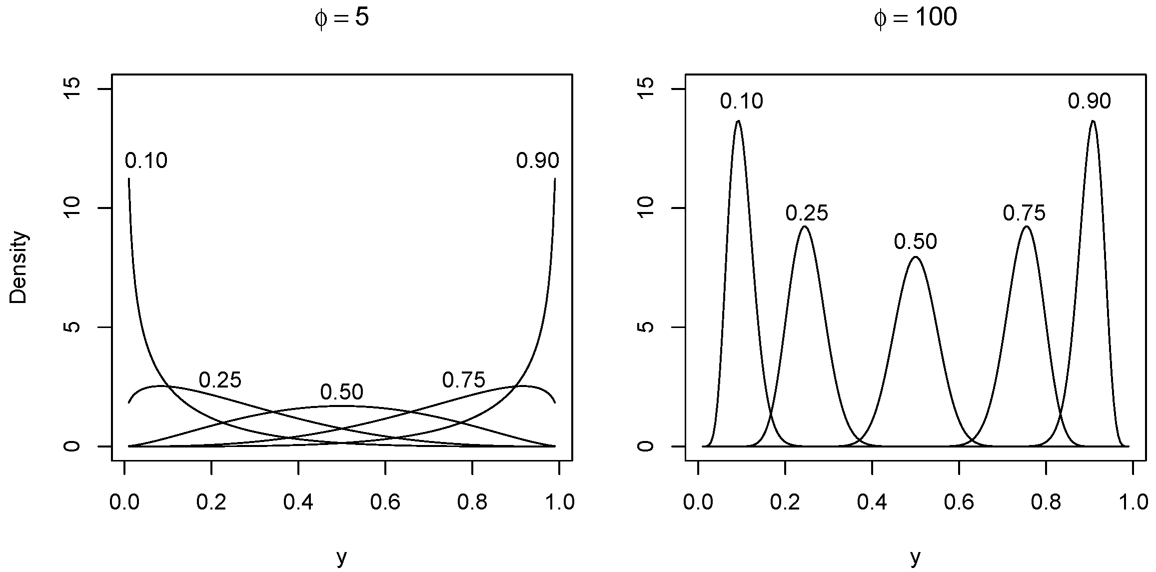In the case of beta models, a suitable choice of g is the logit function formulated as $g\left(\mu \right)=log(\mu /(1-\mu \left)\right)$ and used in generalized linear models [22], which allows the mean to be formulated as:

$${\mu }_t=\frac{exp\left({\mathit{x}}_t^{\top }\mathit{\beta }\right)}{1+exp\left({\mathit{x}}_t^{\top }\mathit{\beta }\right)}.$$

(5)

Note that the expression given in (5) is similar to logistic regression models based on the binomial distribution to describe proportions/percentages [23]. These models are suitable only if the outcome is of the form r out of N (with $y=r/N$). However, this is inapplicable in situations where the raw numbers r and N are not available.

Let $\mathit{Y}={(Y_1,\cdots ,Y_n)}^{\top }$ be independent random variables, where each $Y_t$, for $t\in \{1,\cdots ,n\}$, follows a beta distribution with mean ${\mu }_t$ defined in (5) and PDF stated as in (3). In addition, $\mathit{y}={(y_1,\cdots ,y_n)}^{\top }$ are the observed values of $\mathit{Y}$ and, as mentioned $x_{t1},\cdots ,x_{tk}$ are observations of k fixed covariates, for $k<n$. Then, the log-likelihood function for $\mathit{\theta }={({\beta }_1,\cdots ,{\beta }_k,\varphi )}^{\top }$ based $\mathit{y}$ is expressed as:

$$\ell (\mathit{\theta };\mathit{y})=\ell \left(\mathit{\theta }\right)=\sum _{t=1}^n{\ell }_t\left(\mathit{\theta }\right),$$

(6)

where

$${\ell }_t\left(\mathit{\theta }\right)=log(\Gamma \left(\varphi \right))-log(\Gamma \left({\mu }_t\varphi \right))-log(\Gamma \left((1-{\mu }_t)\varphi \right))+({\mu }_t\varphi -1)log\left(y_t\right)+\left((1-{\mu }_t)\varphi -1\right)log(1-y_t).$$

Therefore, when maximizing the log-likelihood function defined in (6), we obtain the ML estimator of $\mathit{\theta }$. Under mild standard regularity conditions (for example, the conditions described in [24] (Sections 7.1 and 7.2)), the ML estimator of $\mathit{\theta }$ is consistent and asymptotically normal, whereas the log-likelihood function defined in (6) is strictly concave [25]. Note that the ML estimator of $\mathit{\theta }$ does not have a closed form [26]. Hence, they need to be obtained by numerically maximizing the log-likelihood function using nonlinear optimization methods such as Newton or quasi-Newton algorithms [27]. Nonetheless, this ML estimator is biased in small sample size [19,28], but its bias decreases as the sample size increases, which justifies the search for alternative non-linear optimization algorithms.

The beta regression model can be extended to cover different sources of heterogeneity, including non-constant dispersion and non-linearity [29,30,31], temporal dependence [32,33,34,35], inflated points [36,37], truncation [38], and error-in-variables as well as latent information [39,40,41,42], among others. To keep a clear focus, in the present study, we restrict our attention primarily to the fixed precision. Our presentation, however, is not critically dependent on the fixed precision assumption and the simulation results can be increased over other scenarios in future works.

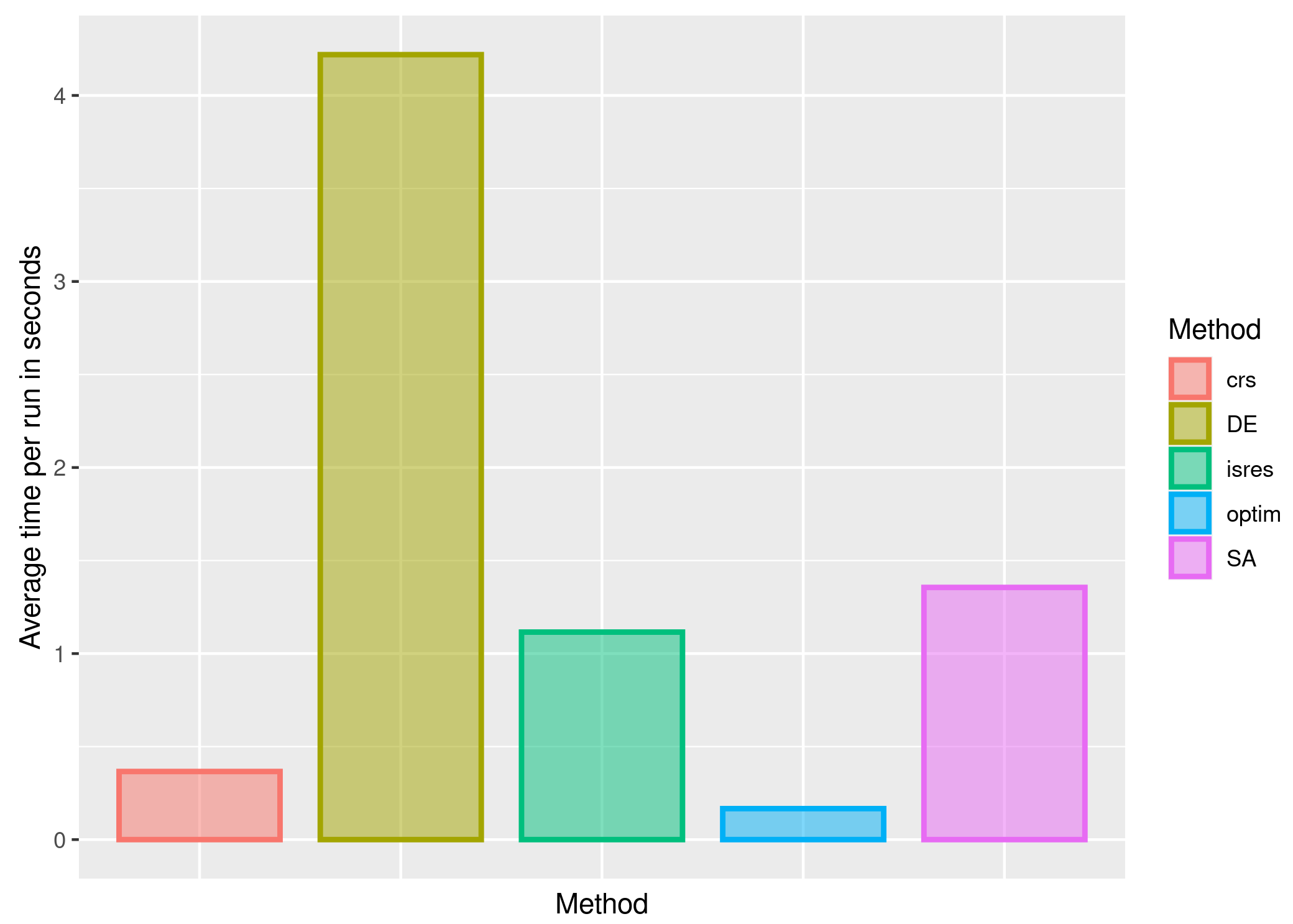
2.2. Optimization Algorithms

As mentioned, it is possible to estimate the parameters of the beta regression model by maximizing the log-likelihood function defined in (6). To do this, several optimization methods can be used, such as heuristics that aim to find satisfactory solutions in viable computational time. These methods are generally effective for highly complex computational problems, such as the one of interest in this investigation.

Monte Carlo simulations considered in this study are divided into two steps. The first step is more general, allowing us to evaluate a large number of methods, selecting those that provide better computational results. The second step aims to compare the previously selected methods with the most employed one by the command optim of R from the betareg package.

The authors in [43] evaluated the 18 optimization methods available in the R language applied to 48 different optimization problems with known solutions. In our case and during the first step, we carry out a simulation study considering only the problem of maximizing the log-likelihood function defined in (6), with 10 different methods available in R packages. In the second stage, we use the methods that provided better results in the previous stage and the optim function implemented in the betareg package, in order to make a comparison. The methods utilized are defined as follows:

• Genetic algorithm: This is a heuristic inspired by the basic principle of biological evolution and natural selection, simulating evolution so that the fittest individuals survive, imitating its mechanisms such as the processes of selection, crossing, and mutation. The ga function that implements this algorithm is available in an R package named GA [44].
• Differential evolutionary algorithm: This method is similar to the genetic algorithm indicated to find the global optimum of real-valued functions with real-valued parameters as well [45]. Such an algorithm does not need the function to be optimized that is continuous or differentiable and is available by the DEoptim command of an R package named DEoptim [46].
• Self-adapted evolutionary algorithm: This method proposed in [47] is a strategy of self-adaptation of the covariance matrix that is implemented in the cma_es function of the cmaes package of R. This is also an evolutionary method, which uses a covariance matrix approximation to be more efficient in the generation of next generations.
• Simulated annealing algorithm: This is a metaheuristic based on the thermodynamic annealing process that performs a probabilistic local search replacing the current solution with a solution in its vicinity, obtaining good solutions regardless of the chosen starting point. The GenSA function is available in an R package named GenSA [48]. A general strategy to improve the simulated annealing (SANN) algorithm is to inject noise via the Markov chain Monte Carlo algorithms (noise-boosted) to sample high probability regions of the search space and to accept solutions that increase the search breadth [49,50,51]. Another approach is based on hybridized search gradient methods or genetic algorithms for cases of difficulties in the convergence with SANN [52,53].
• Controlled random search algorithm: This is a direct search heuristic [54] that tries to balance the fulfillment of constraints and convergence by storing possible trial points by the nloptr_crs function. Such a function has implemented this algorithm and is available in an R package named nloptr [55].
• DIRECT algorithm: This is a deterministic method based on the division of the search space into increasingly smaller hyperrectangles and was proposed in [56]. The  nloptr_d function has implemented such an algorithm and is available in the nloptr package of R.
• DIRECT_L algorithm: This is a variation of DIRECT containing certain randomness and was proposed in [57]. The nloptr_d_l function is available in the nloptr package.
• Evolutionary algorithm: A common practice in evolutionary methods is to apply a penalty function to bias the search for viable solutions. This method is a strategy improved by stochastic ranking that proposes a way to eliminate subjectivity in the configuration of penalty parameters and was proposed in [58]. The nloptr_i function implements this algorithm and is available in the nloptr package of R.
• Memetic algorithm: This technique does a search locally combining the evolutionary method with a local search algorithm. The alschains function has implemented this algorithm and is available in the malschains package of R [59].
• Particle swarm algorithm: This is a heuristic that considers the movement of a swarm of particles through the search space, using formulas for position and velocity that depend on the state of other particles. The PSopt function that implements this algorithm is available in an R package named NMOF [60,61,62,63].
• Broyden–Fletcher–Goldfarb–Shanno (BFGS) algorithm: This is a quasi-Newton optimization method that applies analytical gradients for parameter estimation and uses as initial guesses values obtained through an auxiliary linear regression of the transformed response. The BFGS algorithm is employed in the optim function of the betareg package [16].

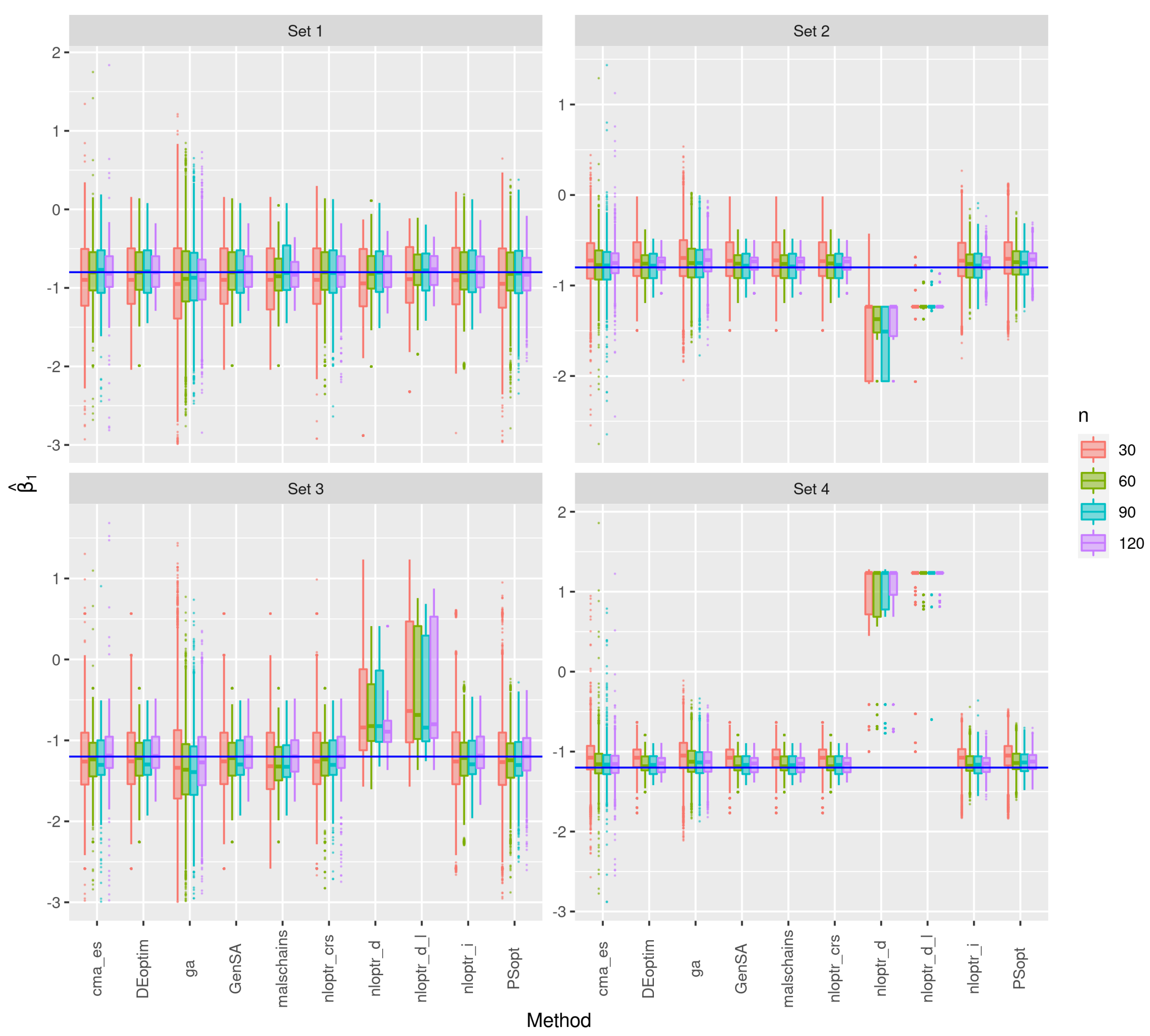
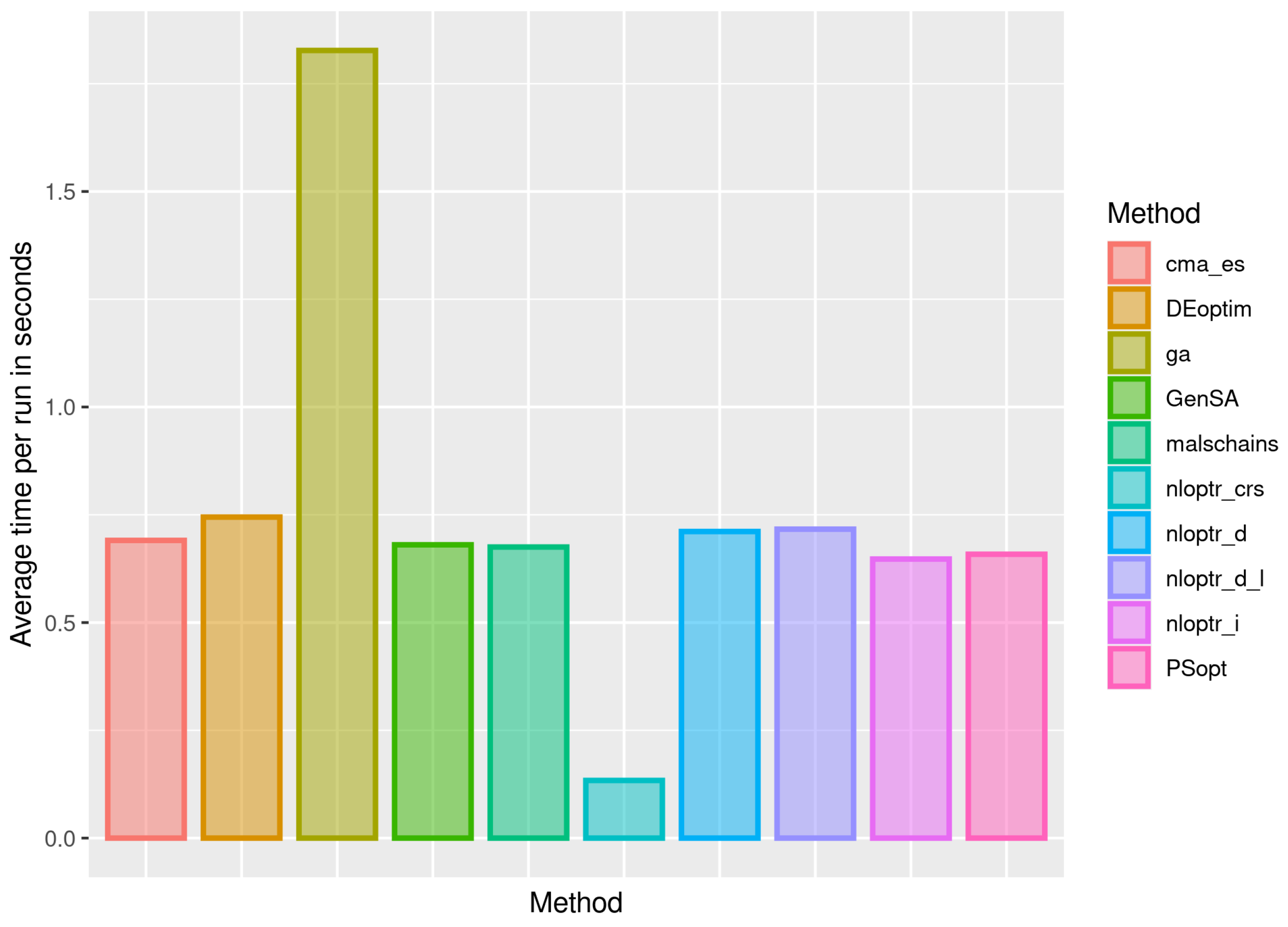
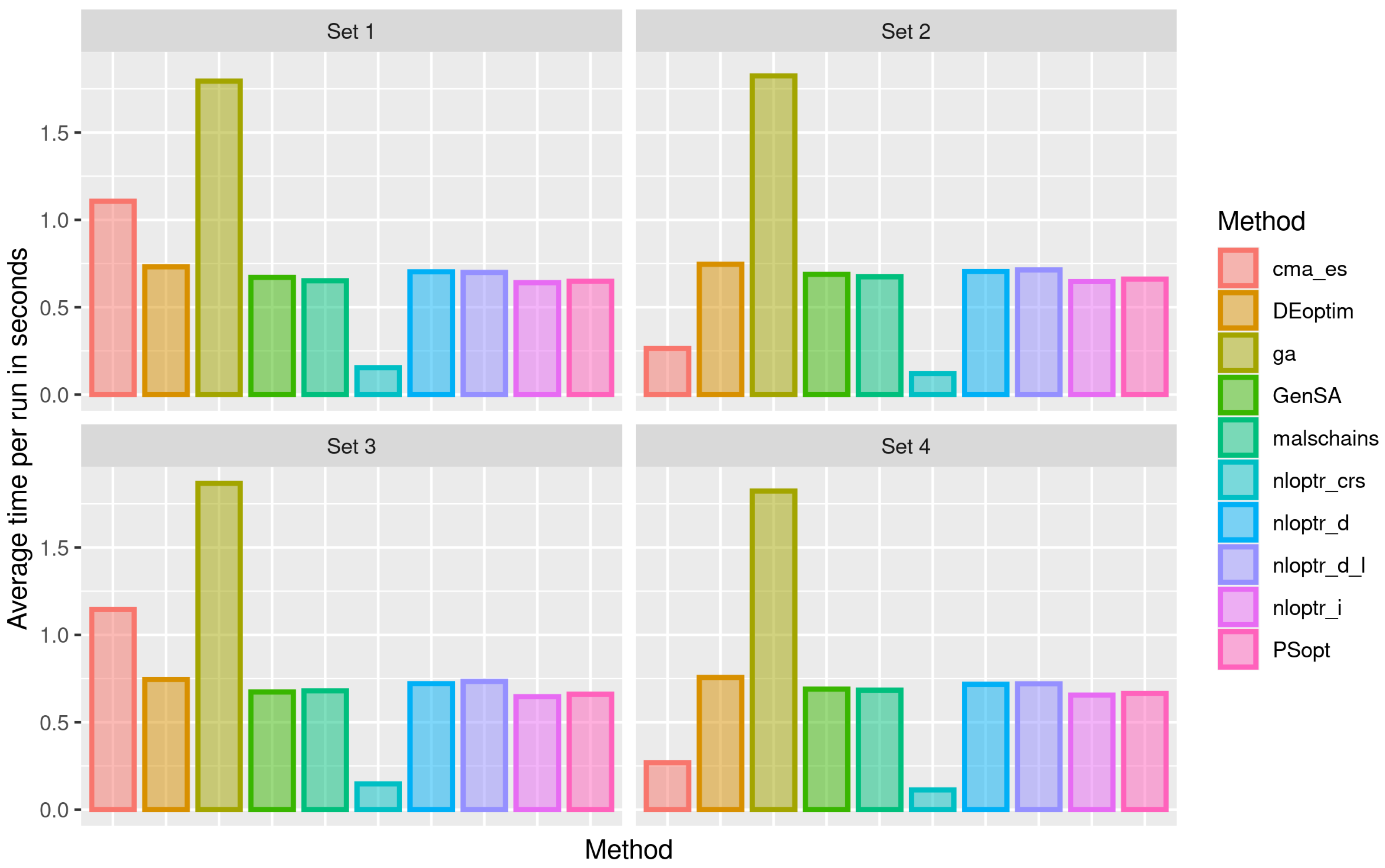
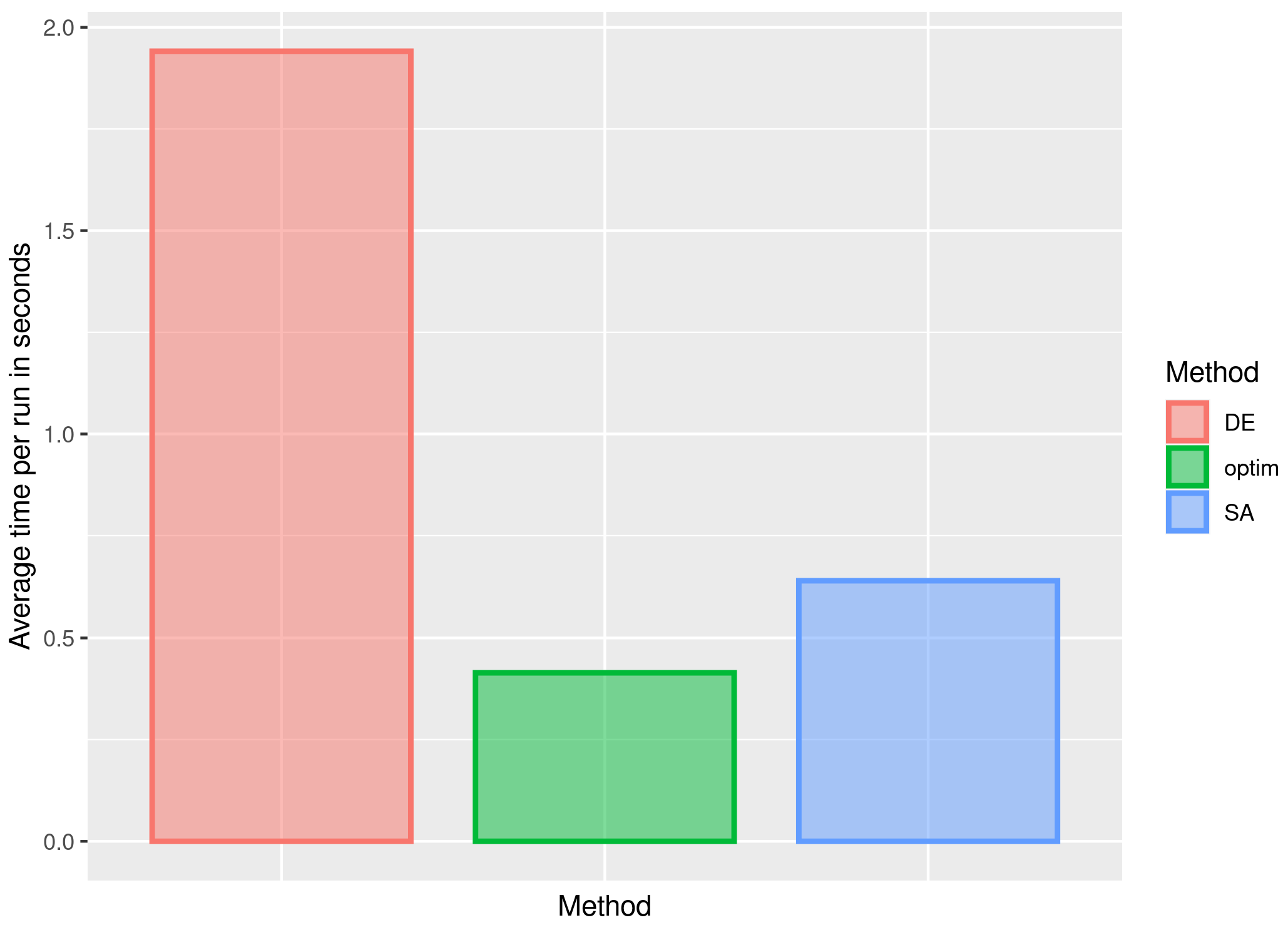
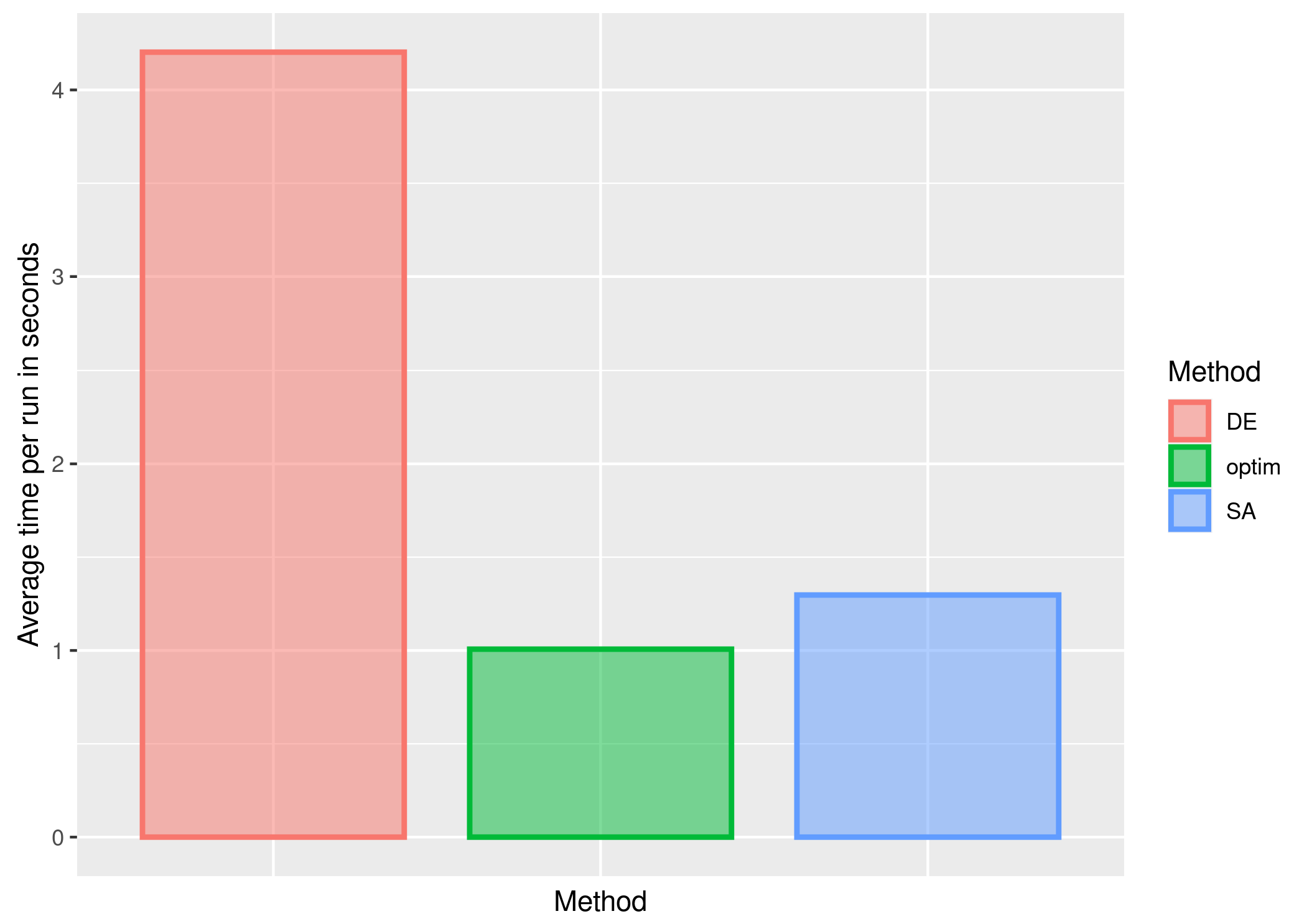
3. Results and Discussion

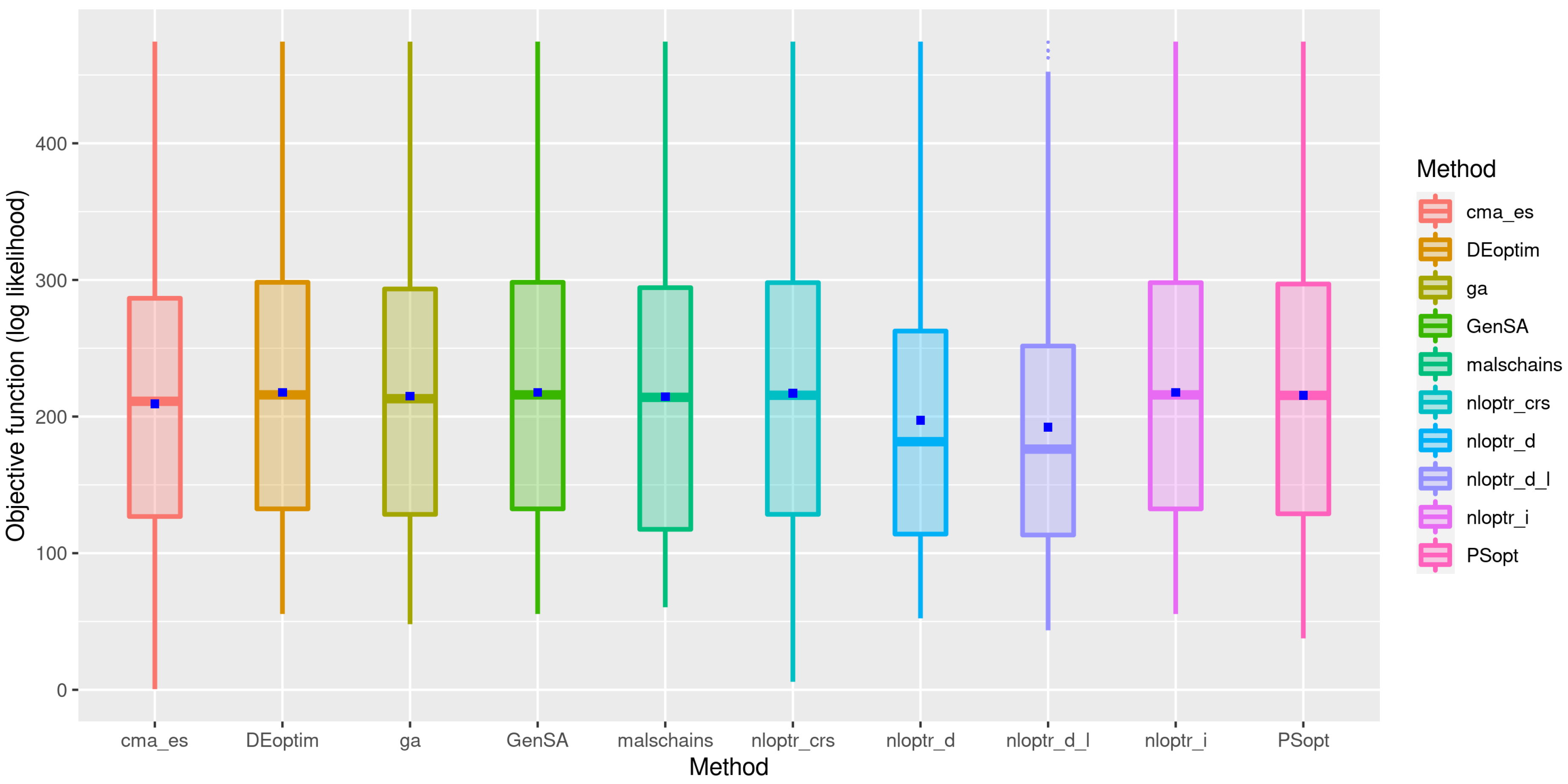
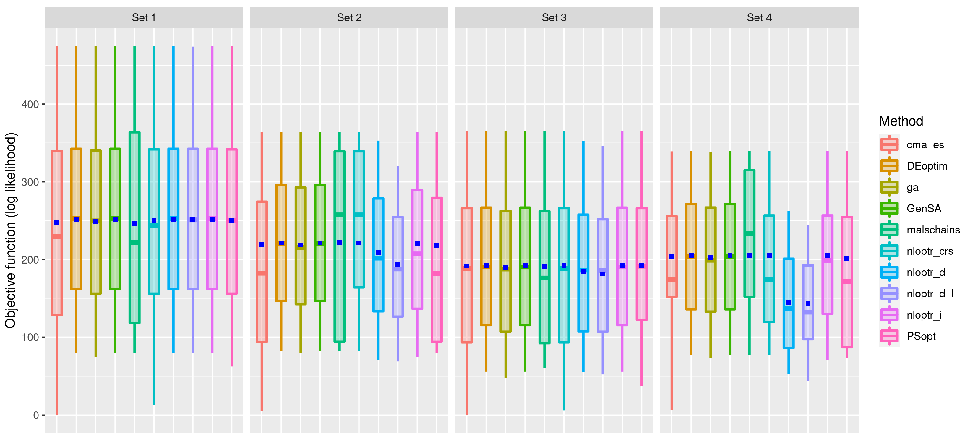
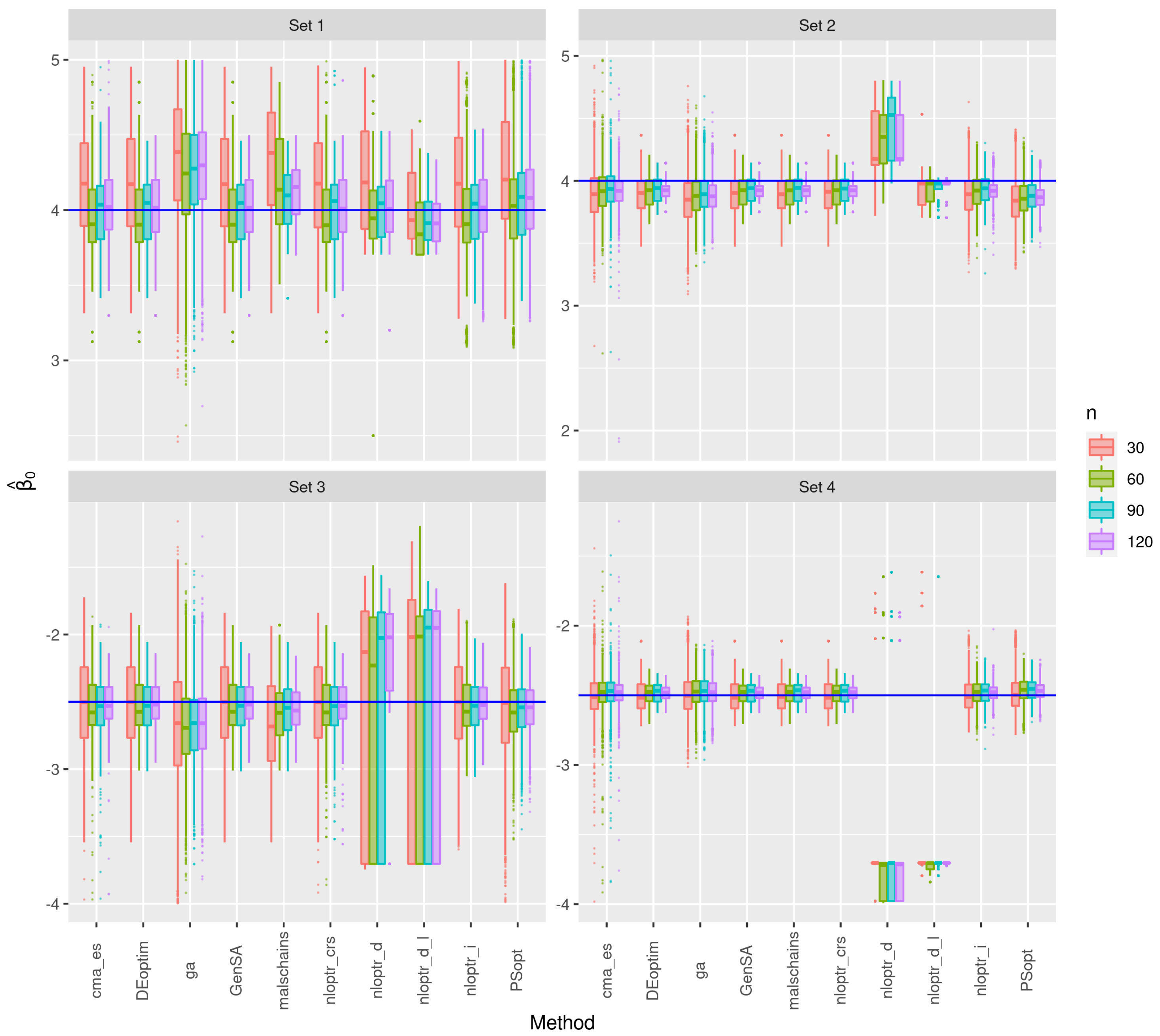
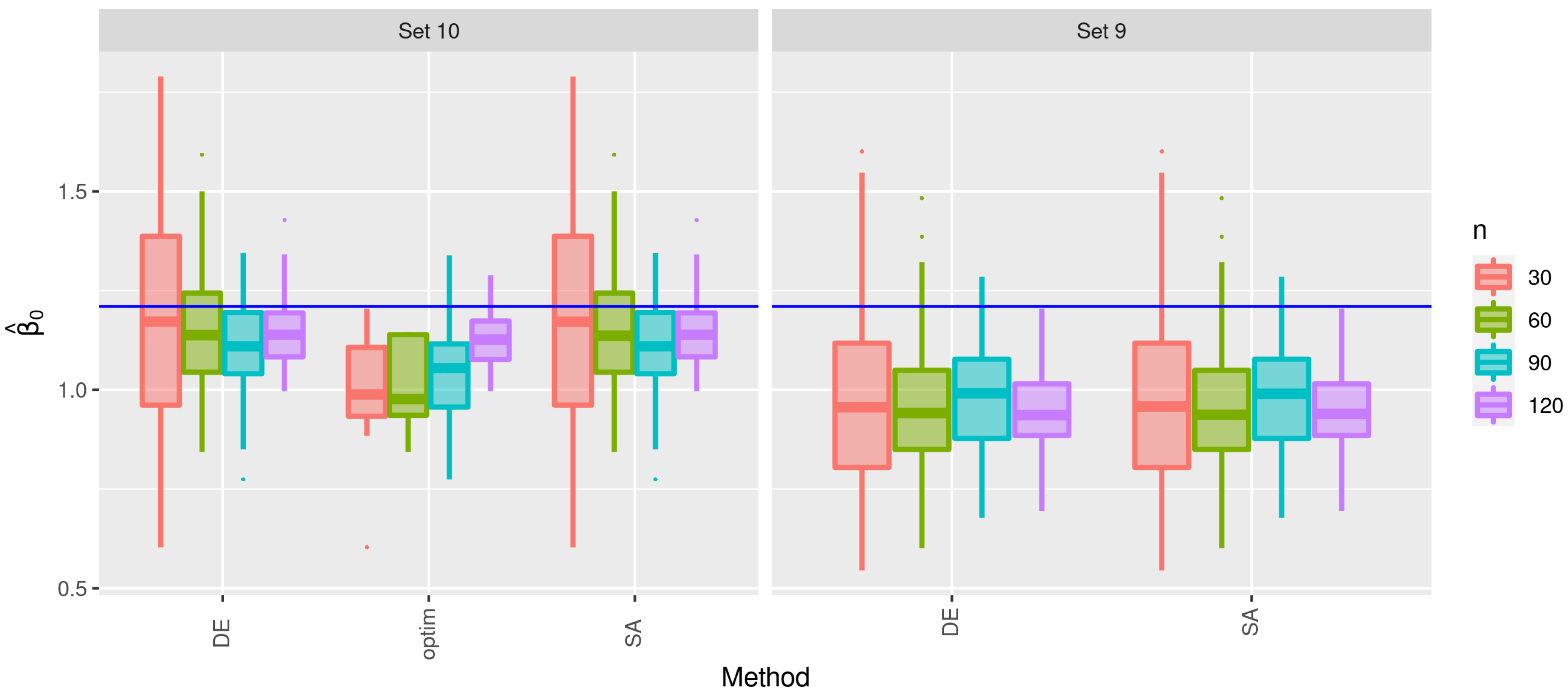
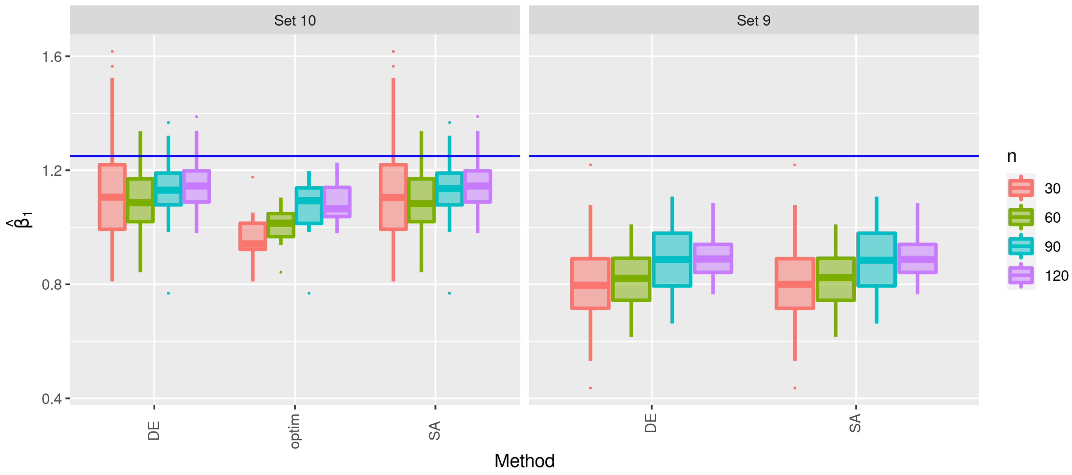
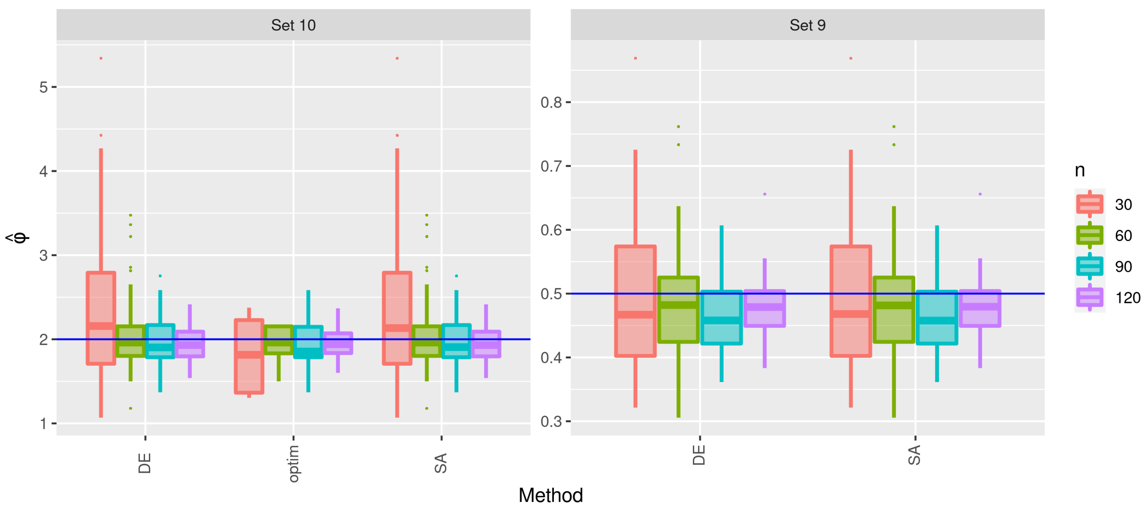
3.1. First Stage of the Simulation

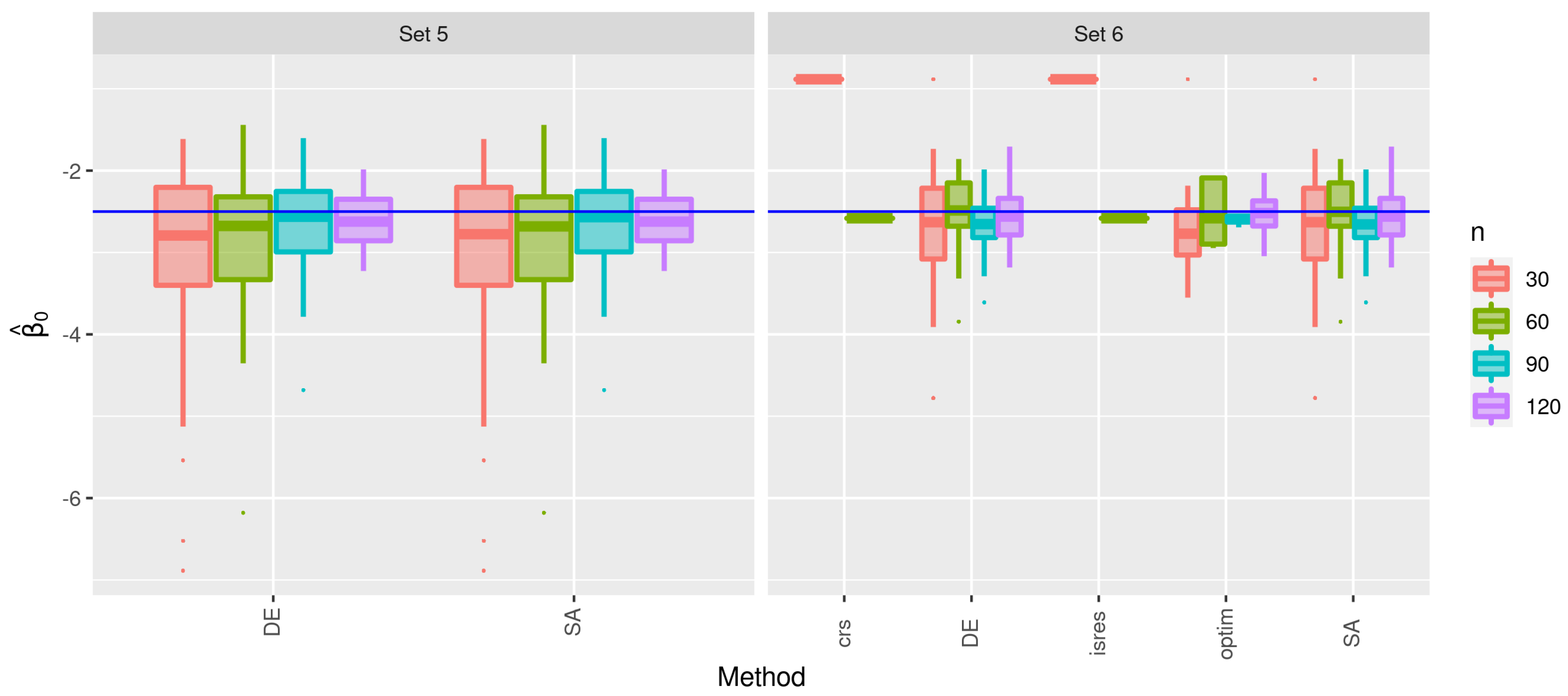
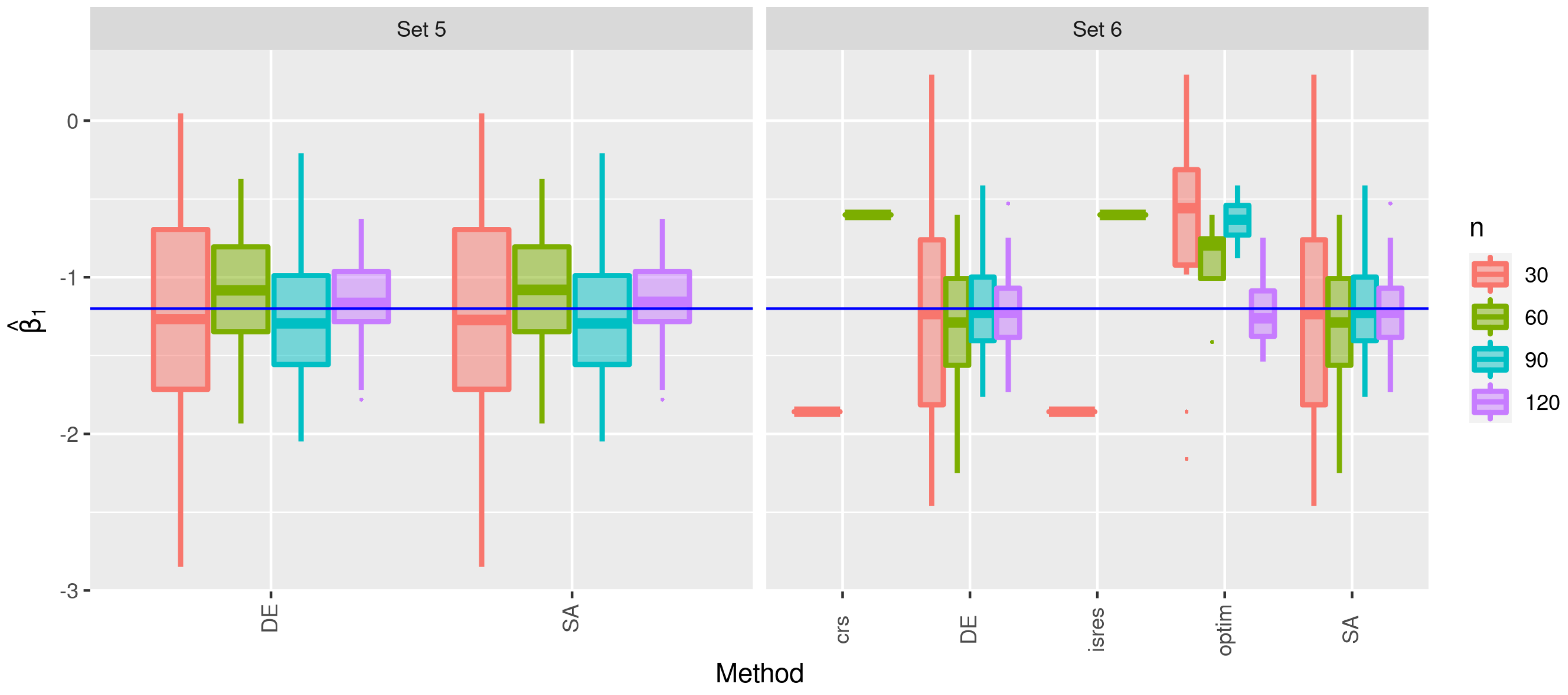
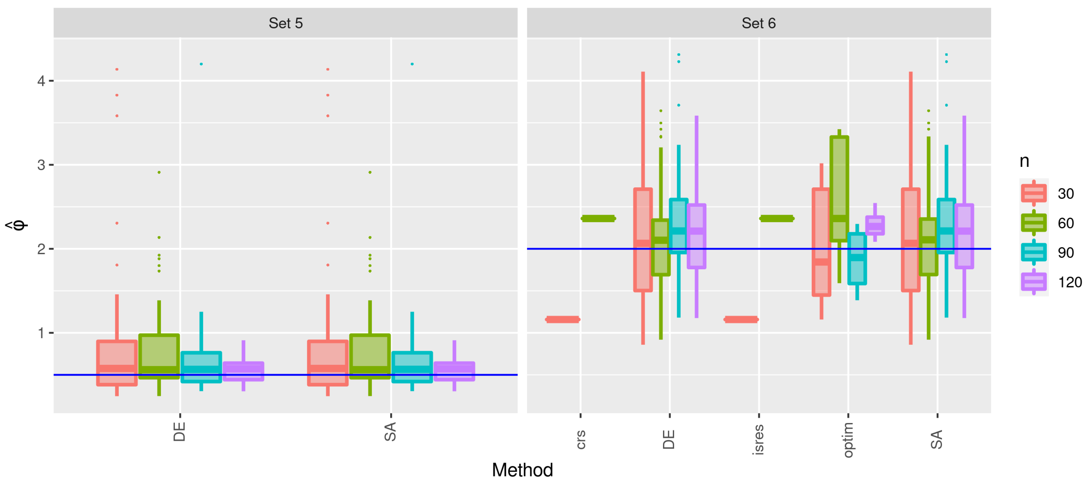
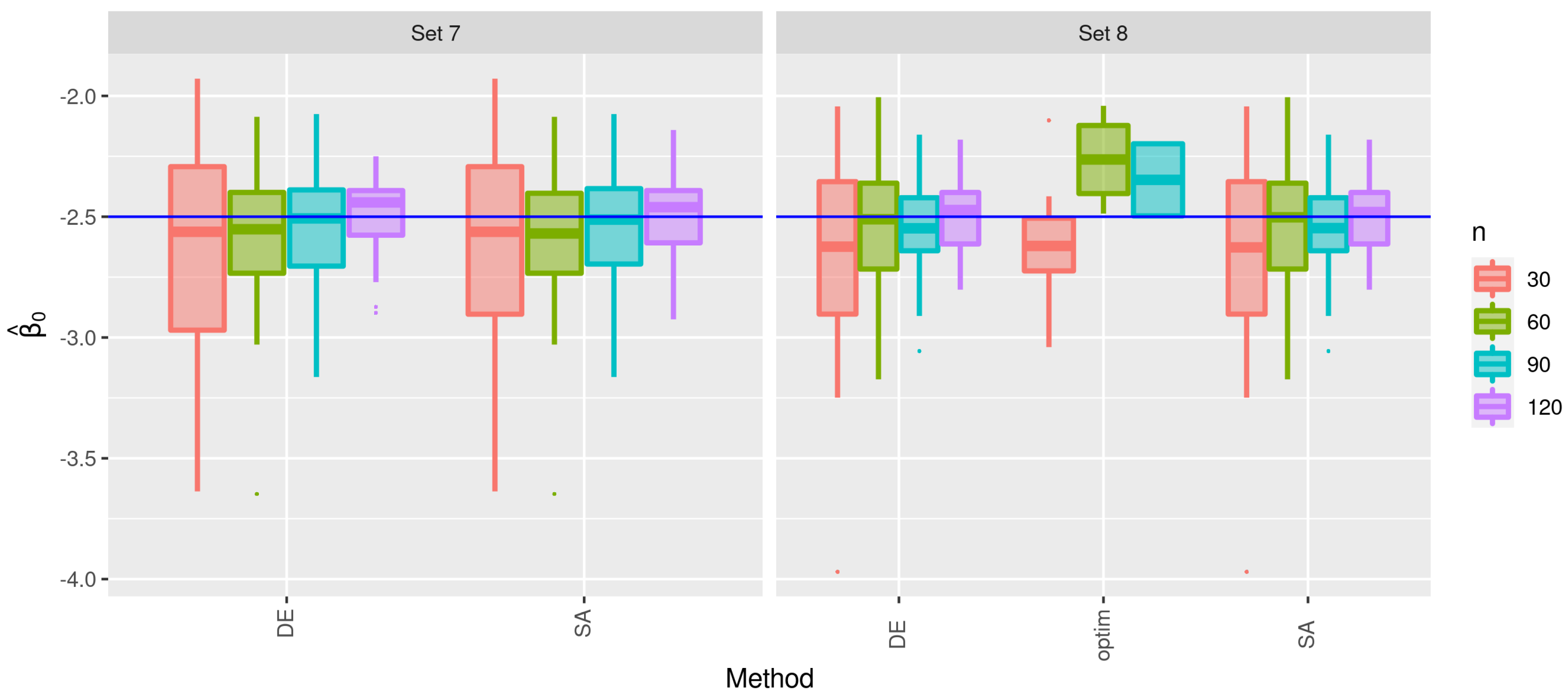
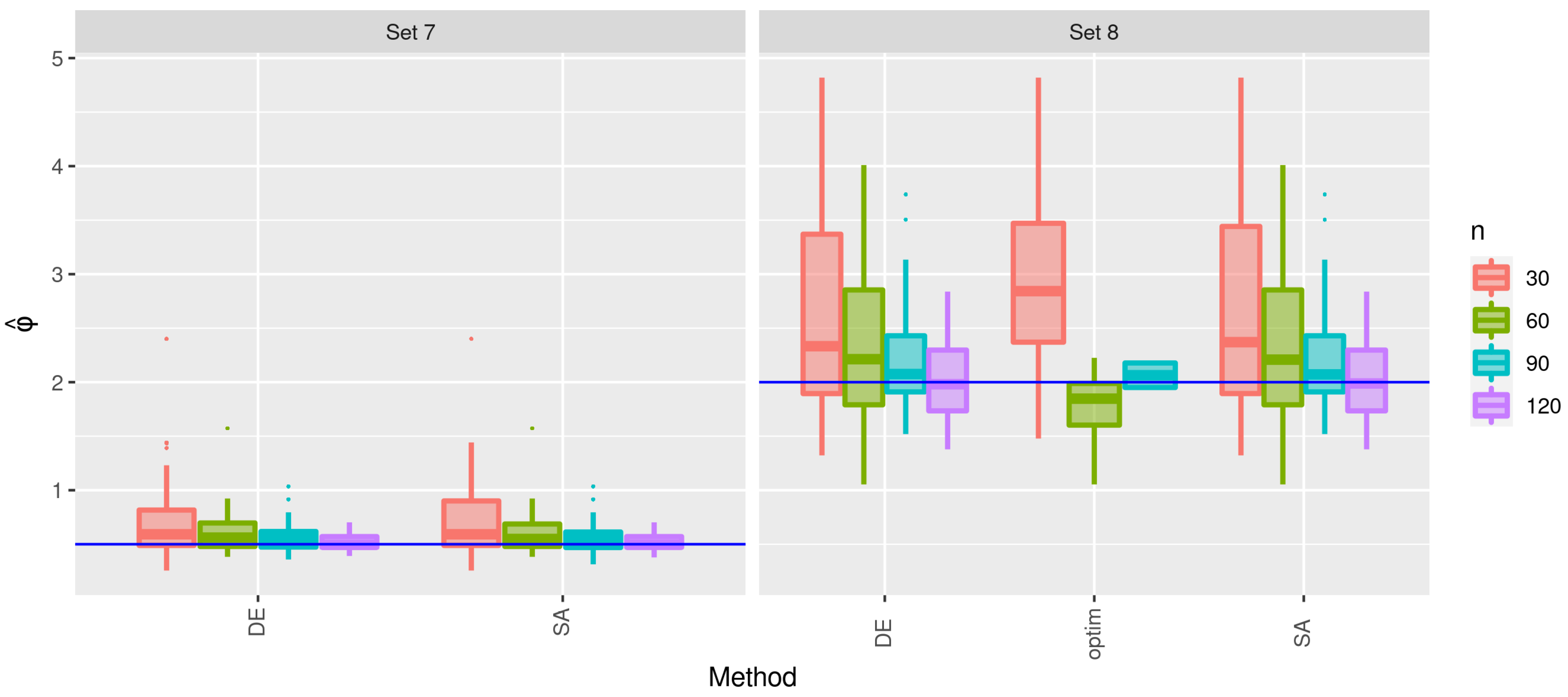
The first stage of the Monte Carlo simulation study was carried out considering the 10 methods mentioned and applied to the estimation of the mentioned beta regression parameters. The data were generated from the beta regression structure with link function $g\left({\mu }_t\right)={\beta }_0+{\beta }_1{x}_t$, such as defined in (4). The values of the covariate $x_t$ were obtained as independent realizations of the uniform distribution, denoted as $\mathrm{Uniform}(0,1)$. Thus, under this structure, we can explore the behavior of the optimization procedures from a challenging vision but in a simple scenario and easy to compute due to the intensive calculations. Therefore, multiple regressions and modeling with varying precision were not considered in the present study and will be considered in future research. Logically, the simulation schemes can be structured using more covariates in mean or precision, including categorical and continuous covariates, nonlinearity, and other linking specifications to evaluate, for example, misspecification and sparsity. Nevertheless, this is beyond the scope of our original work.

Note that, in our study, the matrix of covariates remains constant throughout the experiment. Then, random samples of the response variable $Y_t$ were generated following the beta distribution presented in (3), that is, $Y_t\sim \mathrm{Beta}({\mu }_t,\varphi )$. Four different sets of parameter values were considered as stated in

Table 1. Parameter values for the indicated set used in the simulation study.

	Parameter
Set	${\mathit{\beta }}_0$	${\mathit{\beta }}_1$	$\mathit{\varphi }$
1	$4.0$	$-0.8$	12
2	$4.0$	$-0.8$	148
3	$-2.5$	$-1.2$	12
4	$-2.5$	$-1.2$	148

, where Sets 1 and 2 result in average response values close to one, while Sets 3 and 4 report these values close to zero. For example, ${\beta }_0=-2.5$ and ${\beta }_1=-1.2$ result in mean response values close to zero, $\mu \in (0.024,0.075)$ and, for $\varphi =5$, a beta PDF is induced close to the inverted “J”-shape (asymptotes at zero). This situation is an extreme scenario, where traditional optimization procedures generally fail as shown in [64]. The sample sizes used were $n\in \{30,60,90,120\}$. For each sample size, 50 instances were generated and, for each instance, 100 replicates of each method were performed. Thus, we got 80,000 observations per method. The number of iterations and other method control parameters were adjusted to allow a maximum of 10,000 function calls. Among the 10 evaluated methods, three of them returned an error in some replicates, without providing any result. These methods and the number of failures are shown in

Table 2. Indicators of failures for the listed method.

	Method
Indicator	cma_es	malschains	PSopt
Number of failures	$39.03$	$33.90$	$7.06$
Percentage of failures	$48.78\%$	$42.37\%$	$8.82\%$

. The seven remaining methods did not return any error.

The performance of methods can be further visualized with box plots summarizing the main statistical properties of the measures. The bar in each box is the median value of the measure across the runnings, while outliers deviating by one or more quartiles from the median are denoted as discrete dots at the extremes (outliers). Figure 2 displays the values obtained of the overall log-likelihood function corresponding with each method through box plots. With the exception of the nloptr_d and nloptr_d_l methods, the other algorithms obtained similar results to each other.

Figure 3 shows the performance in terms of the values of the log-likelihood function corresponding to the beta regression mean for each of the four sets described in Table 1. For the first set of parameters, most methods seem to have a similar performance, with the exception of the malschains and cma_es methods. In the second set, the nloptr_crs and malschains methods stand out from the rest. In the third set, there is a certain heterogeneity in the estimates, whereas for the fourth set, the malschains method stands out again, with the nloptr_d and nloptr_d_l methods being quite different from the others. Although the malschains method seems to perform well in some sets, it has some inconsistency with 33,900 failed executions, which are about $42\%$.

Figure 4 presents the box plots of the intercept estimates (${\beta }_0$) for each method, separated by parameter set and sample size, where the blue line indicates the real value of the parameter to be estimated. Such estimates seem to be more accurate as the sample size increases, as expected. The nloptr_d and nloptr_d_l methods report large variations in the results, which is evident in the graphical plot of Set 3. Note that the ga and cma_es methods present a large number of outliers in most sets. The other methods seem to behave similarly to each other, obtaining estimates close to the expected value.

The box plots of the estimates of the parameter ${\beta }_1$, separating by parameter set and sample size, are shown in Figure 5, where once again the blue line indicates the real value of the parameter to be estimated. The results are very similar to those obtained in Figure 4, since again the nloptr_d and nloptr_d_l methods present large variations in the results and the ga and cma_es methods show a large number of outliers, while the rest of the methods obtained similar results, approaching the blue line. Again, an approximation of the estimates in relation to the blue line is observed as the sample size increases.

In addition to the quality of the estimates, it is of interest to assess the speed of the methods to obtain them. Figure 6 shows a bar plot of the average time per execution in seconds for each method. The ga algorithm is the slowest one, taking more than 1.5 s per run. The nloptr_crs method is much faster than all the others. The other methods have a similar speed performance to each other.

Figure 7 sketches the bar plots of the average time per execution in seconds, for each method, separated by a set of parameters. Observe that the execution speed behavior does not seem to depend on the set of parameters to be estimated, with the exception of the cma_es method, which was much slower when dealing with estimates for $\varphi =148$.

Given these results, the DEoptim, GenSA, nloptr_i, and nloptr_crs methods seem to be the most suitable, as the malschains, nloptr_d, nloptr_d_l, PSopt, ga, and cma_es methods show some inconsistencies in the parameter estimation.

3.2. Second Stage of the Simulation

In this step, the same methodology as the previous step is used, considering only the methods that have previously obtained better results (DE, SA, isres, crs) and the optim function currently utilized in the betareg package. Thus, it is possible to compare how the heuristics behave in relation to the currently most employed method, that is, the optim function of the betareg package. Furthermore, sets are investigated in which the methods are expected to have greater difficulty in estimating the parameters, diversifying the distribution of the covariate to the cases: Uniform(0,1); Normal(0,1); and Student-t(3). Note that the value of the precision parameter $\varphi$ drastically decreases as the variance increases. The configuration used for the generated samples is found in

Table 3. Parameter sets used in the second stage of the simulation.

		Parameter
Set	Distribution	${\mathit{\beta }}_0$	${\mathit{\beta }}_1$	$\mathit{\varphi }$
5	Uniform(0,1)	$-2.50$	$-1.20$	$0.5$
6	Uniform(0,1)	$-2.50$	$-1.20$	$2.0$
7	Normal(0,1)	$-2.05$	$-1.20$	$0.5$
8	Normal(0,1)	$-2.50$	$-1.20$	$2.0$
9	Student-t(3)	$1.21$	$1.25$	$0.5$
10	Student-t(3)	$1.21$	$1.25$	$2.0$

. Note that, in

Table 4. Indicators of failures for the listed method with Sets 5 and 6 of the second stage of the simulation.

		Method
Sets	Indicator	crs	DEoptim	isres	optim	GenSA
5–6	Number of failures	$39.83$	0	$39.80$	$37.50$	19
	Percentage of failures	$99.56\%$	$0\%$	$99.50\%$	$93.75\%$	$0.04\%$
7–8	Number of failures	$39.83$	0	$39.80$	$37.50$	19
	Percentage of failures	$99.56\%$	$0\%$	$99.50\%$	$93.75\%$	$0.04\%$
9–10	Number of failures	$39.83$	0	$39.80$	$37.50$	19
	Percentage of failures	$99.56\%$	$0\%$	$99.50\%$	$93.75\%$	$0.04\%$

, for Sets 5 and 6, only the DEoptim and GenSA methods can consistently estimate the parameters based on the number of failures per method.

In Figure 8, the box plots of the estimates of ${\beta }_0$ for Sets 5 and 6 are presented. Note that, for Set 5, only the DE and SA methods reported successes, whereas for Set 6, the isres, crs, and optim methods had few successes. This result is consistent with the number of failures shown in Table 4. Furthermore, the estimates performed with the DE and SA methods are similar. For the same sets, in Figure 9, the box plots of the estimates of ${\beta }_1$ are displayed, where similar behavior is detected, with the notable difference that, in this case, the optim function provides more heterogeneous results in the case of samples with small sizes. The estimates of $\varphi$ are shown in Figure 10, where a similar behavior is observed in relation to the estimates of ${\beta }_0$ and ${\beta }_1$.

For Sets 7 and 8, observe that, in Table 4, the crs and isres methods failed in all attempts, while the optim function failed in most executions. In addition, the DE and SA methods had few flaws/failures, being the most consistent algorithms. The estimates of ${\beta }_0$ shown in Figure 11 report that the behavior remains similar between the DE and SA methods. Note that the optim function did not have any success in estimating the parameters for samples of size $n=120$. The same can be seen in the estimates of ${\beta }_1$ in Figure 12 and in the estimates of $\varphi$ in Figure 13.

For Sets 9 and 10, observe that, in Table 4, once again the crs and isres methods are unable to provide estimates. In this case, the optim function had a lower number of failures, although it is still a considerably significant number. The DE method follows without failing, while the SA method reports some few flaws. Figure 14, Figure 15 and Figure 16 show the estimates of ${\beta }_0$, ${\beta }_1$, and $\varphi$, respectively. In this case, the optim function did not obtain estimates for Set 9. Furthermore, a similar behavior between the DE and SA methods is confirmed. Note that the estimates of ${\beta }_1$ were not very accurate for Set 9.

For Sets 5 and 6, Figure 17 sketches the average execution time in seconds, considering only the successes. Note that, despite the large number of failures, the optim function is quite efficient when it comes to estimating the parameters. Although the DE and SA methods have obtained close estimates, the execution time of the SA method is much smaller, so that its use is indicated in the studied cases. For Sets 7 and 8, as previously shown in Figure 18, it is confirmed that the execution time of the SA method is less than for the DE method, despite the similarity in the estimates. For Sets 9 and 10, as for the execution times shown in Figure 19, the previous behavior is once again detected, with the SA method being more efficient than the DE method.

4. Conclusions

This work evaluated the performance of the most used optimization methods when numerically maximizing the likelihood function associated with the beta regression model for different scenarios, varying the distribution of the covariate, its parameters, and sample size.

We considered a Monte Carlo simulation study in two stages. From the results of the first stage of these simulations carried out and the analysis of the graphical plots presented, we observed that six methods reported some inconsistencies and were not suitable for the problem. These methods are the genetic, evolutionary with self-adaptation of the covariance matrix, DIRECT, DIRECT_L, memetic with local search strings, and particle swarm algorithms. Four other methods provided satisfactory results, that is, the differential evolutionary, simulated annealing, controlled random search, and evolutionary with improved stochastic ranking algorithms. All of them obtained similar and satisfactory results in relation to the estimates in the evaluated scenarios. However, among them, the controlled random search algorithm had a superior computational speed performance in relation to the others. In the second stage of the simulations, sets of parameters were used to make the estimation process more difficult. In this case, we observed that the controlled random search and evolutionary with improved stochastic ranking algorithms presented a very large number of failures, in some cases not achieving any success. The optim function used in the betareg package of R had many failures, but in cases where it was successful, it outperformed the other methods both in terms of accuracy of estimation and speed. The differential evolutionary and simulated annealing algorithms provided satisfactory estimates with few failures, with the simulated annealing algorithm being more efficient in terms of computational time.

Based on the findings detected in our computational study, we report the following. The optim function, implemented in the betareg package to maximize the log-likelihood function of the beta regression model and to estimate its parameters, is accurate and efficient for most of the cases. Nevertheless, in some scenarios reported in our study, it presents some difficulties in estimating such parameters. In these scenarios, we recommend the use of the simulated annealing algorithm, which for the cases studied in this work showed greater consistency, providing satisfactory estimates in viable computational time.

Some limitations of our investigation, which open naturally the possibility of future works, are related to investigating the case of a varying precision parameter by means of a regression structure to $log\left({\varphi }_t\right)$. In addition, since we used one covariate in the simulation study, an exploration of experimental results in the case of multiple regression is of interest because could affect the results. These open problems and others that are related are suitable to be further analyzed so that we hope to report their findings in a future publication.

References

- Berggren, N.; Daunfeldt, S.O.; Hellström, J. Social trust and central-bank independence. Eur. J. Political Econ. 2014, 34, 425–439. [Google Scholar] [CrossRef] [Green Version]
- Buntaine, M.T. Does the Asian development bank respond to past environmental performance when allocating environmentally risky financing? World Dev. 2011, 39, 336–350. [Google Scholar] [CrossRef]
- Castellani, M.; Pattitoni, P.; Scorcu, A.E. Visual artist price heterogeneity. Econ. Bus. Lett. 2012, 1, 16–22. [Google Scholar] [CrossRef] [Green Version]
- De Paola, M.; Scoppa, V.; Lombardo, R. Can gender quotas break down negative stereotypes? Evidence from changes in electoral rules. J. Public Econ. 2010, 94, 344–353. [Google Scholar] [CrossRef]
- Huang, X.; Oosterlee, C. Generalized beta regression models for random loss-given-default. J. Credit. Risk 2011, 7, 1–27. [Google Scholar] [CrossRef] [Green Version]
- Figueroa-Zúniga, J.; Bayes, C.L.; Leiva, V.; Liu, S. Robust beta regression modeling with errors-in-variables: A Bayesian approach and numerical applications. Stat. Pap. 2022. [Google Scholar] [CrossRef]
- Martinez-Florez, G.; Leiva, V.; Gomez-Deniz, E.; Marchant, C. A family of skew-normal distributions for modeling proportions and rates with zeros/ones excess. Symmetry 2020, 12, 1439. [Google Scholar] [CrossRef]
- Mazucheli, J.; Bapat, S.R.; Menezes, A.F.B. A new one-parameter unit Lindley distribution. Chil. J. Stat. 2019, 11, 53–67. [Google Scholar]
- Huerta, M.; Leiva, V.; Lillo, C.; Rodriguez, M. A beta partial least squares regression model: Diagnostics and application to mining industry data. Appl. Stoch. Model. Bus. Ind. 2018, 34, 305–321. [Google Scholar] [CrossRef]
- Figueroa-Zúniga, J.; Niklitschek, S.; Leiva, V.; Liu, S. Modeling heavy-tailed bounded data by the trapezoidal beta distribution with applications. Revstat, 2022, in press.
- Smithson, M.; Verkuilen, J. A better lemon squeezer? Maximum-likelihood regression with beta-distributed dependent variables. Psychol. Methods 2006, 11, 54–71. [Google Scholar] [CrossRef] [Green Version]
- Cribari-Neto, F.; Souza, T.C. Religious belief and intelligence: Worldwide evidence. Intelligence 2013, 41, 482–489. [Google Scholar] [CrossRef]
- Souza, T.C.; Cribari-Neto, F. Intelligence and religious disbelief in the united states. Intelligence 2018, 68, 48–57. [Google Scholar] [CrossRef]
- Mazucheli, M.; Leiva, V.; Alves, B.; Menezes, A.F.B. A new quantile regression for modeling bounded data under a unit Birnbaum–Saunders distribution with applications in medicine and politics. Symmetry 2021, 13, 682. [Google Scholar] [CrossRef]
- Ferrari, S.; Cribari-Neto, F. Beta regression or modeling rates and proportions. J. Appl. Stat. 2004, 31, 799–815. [Google Scholar] [CrossRef]
- Cribari-Neto, F.; Zeileis, A. Beta regression in R. J. Stat. Softw. 2010, 34, 1–24. [Google Scholar] [CrossRef] [Green Version]
- Paolino, P. Maximum likelihood estimation of models with beta-distributed dependent variables. Political Anal. 2001, 9, 325–346. [Google Scholar] [CrossRef]
- Cribari-Neto, F.; Vasconcellos, K. Nearly unbiased maximum likelihood estimation for the beta distribution. J. Stat. Comput. Simul. 2002, 72, 107–118. [Google Scholar] [CrossRef]
- Ospina, R.; Cribari-Neto, F.; Vasconcellos, K. Improved point and interval estimation for a beta regression model. Comput. Stat. Data Anal. 2006, 51, 960–981. [Google Scholar] [CrossRef]
- R Core Team. R: A Language and Environment for Statistical Computing; R Foundation for Statistical Computing, Vienna, Austria. 2021. Available online: https://www.R-project.org (accessed on 6 January 2022).
- Dunn, P.K.; Smyth, G.K. Generalized Linear Models with Examples in R; Springer: New York, NY, USA, 2018. [Google Scholar]
- McCullagh, P.; Nelder, J.A. Generalized Linear Models; Chapman and Hall: London, UK, 1989. [Google Scholar]
- Hilbe, J. Logistic Regression Models; Chapman and Hall: New York, NY, USA, 2009. [Google Scholar]
- McCullagh, P. Tensor Methods in Statistics; Chapman and Hall: London, UK, 2018. [Google Scholar]
- Rydlewski, J.; Mielczarek, D. On the maximum likelihood estimator in the generalized beta regression model. Opusc. Math. 2012, 32, 761–774. [Google Scholar] [CrossRef]
- Simas, A.; Barreto-Souza, W.; Rocha, A.V. Improved estimators for a general class of beta regression models. Comput. Stat. Data Anal. 2010, 54, 348–366. [Google Scholar] [CrossRef] [Green Version]
- Rustagi, J. Optimization Techniques in Statistics; Elsevier: Amsterdam, The Netherlands, 2014. [Google Scholar]
- Kosmidis, I.; Firth, D. A generic algorithm for reducing bias in parametric estimation. Electron. J. Stat. 2010, 4, 1097–1112. [Google Scholar] [CrossRef]
- Espinheira, P.; Silva, L.; Silva, A.; Ospina, R. Model selection criteria on beta regression for machine learning. Mach. Learn. Knowl. Extr. 2019, 1, 427–449. [Google Scholar] [CrossRef] [Green Version]
- Grün, B.; Kosmidis, I.; Zeileis, A. Extended beta regression in R: Shaken, stirred, mixed, and partitioned. J. Stat. Softw. 2012, 48, 1–25. [Google Scholar] [CrossRef] [Green Version]
- Rocha, A.; Simas, A.B. Influence diagnostics in a general class of beta regression models. TEST 2011, 20, 95–119. [Google Scholar] [CrossRef]
- Billio, M.; Casarin, R. Beta autoregressive transition Markov-switching models for business cycle analysis. Stud. Nonlinear Dyn. Econom. 2011, 15, 4. [Google Scholar] [CrossRef]
- Pumi, G.; Valk, M.; Bisognin, C.; Bayer, F.; Prass, T. Beta autoregressive fractionally integrated moving average models. J. Stat. Plan. Inference 2019, 200, 196–212. [Google Scholar] [CrossRef] [Green Version]
- Silva, C.; Migon, H.; Correia, L. Dynamic Bayesian beta models. Comput. Stat. Data Anal. 2011, 55, 2074–2089. [Google Scholar] [CrossRef]
- Bayer, F.; Cintra, R.; Cribari-Neto, F. Beta seasonal autoregressive moving average models. J. Stat. Comput. Simul. 2018, 88, 2961–2981. [Google Scholar] [CrossRef] [Green Version]
- Galvis, D.; Bandyopadhyay, D.; Lachos, V. Augmented mixed beta regression models for periodontal proportion data. Stat. Med. 2014, 33, 3759–3771. [Google Scholar] [CrossRef] [PubMed]
- Ospina, R.; Ferrari, S. A general class of zero-or-one inflated beta regression models. Comput. Stat. Data Anal. 2012, 56, 1609–1623. [Google Scholar] [CrossRef] [Green Version]
- Pereira, G.; Botter, D.; Sandoval, M. The truncated inflated beta distribution. Commun. Stat. Theory Methods 2012, 41, 907–919. [Google Scholar] [CrossRef] [Green Version]
- Bonat, W.; Ribeiro, P., Jr.; Zeviani, W. Likelihood analysis for a class of beta mixed models. J. Appl. Stat. 2015, 42, 252–266. [Google Scholar] [CrossRef] [Green Version]
- de Brito Trindade, D.; Espinheira, P.; Pinto Vasconcellos, K.; Farfán Carrasco, J.; Lima, M. Beta regression model nonlinear in the parameters with additive measurement errors in variables. PLoS ONE 2021, 16, e0254103. [Google Scholar] [CrossRef] [PubMed]
- Carrasco, J.; Ferrari, S.; Arellano-Valle, R. Errors-in-variables beta regression models. J. Appl. Stat. 2014, 41, 1530–1547. [Google Scholar] [CrossRef]
- Figueroa-Zúñiga, J.; Arellano-Valle, R.; Ferrari, S. Mixed beta regression: A Bayesian perspective. Comput. Stat. Data Anal. 2013, 61, 137–147. [Google Scholar] [CrossRef] [Green Version]
- Mullen, K.M. Continuous global optimization in R. J. Stat. Softw. 2014, 60, 1–45. [Google Scholar] [CrossRef] [Green Version]
- Scrucca, L. GA: A package for genetic algorithms in R. J. Stat. Softw. 2013, 53, 1–37. [Google Scholar] [CrossRef] [Green Version]
- Dünder, E.; Cengíz, M. Model selection in beta regression analysis using several information criteria and heuristic optimization. J. New Theory 2020, 33, 76–84. [Google Scholar]
- Mullen, K.; Ardia, D.; Gil, D.; Windover, D.; Cline, J. DEoptim: An R package for global optimization by differential evolution. J. Stat. Softw. 2011, 40, 1–26. [Google Scholar] [CrossRef] [Green Version]
- Hansen, N.; Ostermeier, A. Adapting arbitrary normal mutation distributions in evolution strategies: The covariance matrix adaptation. In Proceedings of the IEEE International Conference on Evolutionary Computation, Nagoya, Japan, 20–22 May 1996; pp. 312–317. [Google Scholar] [CrossRef]
- Xiang, Y.; Gubian, S.; Suomela, B.; Hoeng, J. Generalized simulated annealing for efficient global optimization: The GenSA package for R. R J. 2013, 5, 13–21. [Google Scholar] [CrossRef] [Green Version]
- Franzke, B.; Kosko, B. Noise can speed Markov chain Monte Carlo estimation and quantum annealing. Phys. Rev. E 2019, 100, 053309. [Google Scholar] [CrossRef] [PubMed]
- Geyer, C. Markov chain Monte Carlo maximum likelihood. In Computing Science and Statistics, Proceedings of 23rd Symposium on the Interface, Fairfax Station, Seattle, WA, USA, 21–24 April 1991; Interface Foundation of North America: Fairfax Station, VA, USA, 1991; pp. 156–163. [Google Scholar]
- Martino, L.; Elvira, V.; Luengo, D.; Corander, J.; Louzada, F. Orthogonal parallel MCMC methods for sampling and optimization. Digit. Signal Process. 2016, 58, 64–84. [Google Scholar] [CrossRef] [Green Version]
- El-Alem, M.; Aboutahoun, A.; Mahdi, S. Hybrid gradient simulated annealing algorithm for finding the global optimal of a nonlinear unconstrained optimization problem. Soft Comput. 2021, 25, 2325–2350. [Google Scholar] [CrossRef]
- Xu, P.; Sui, S.; Du, Z. Application of Hybrid Genetic Algorithm Based on Simulated Annealing in Function Optimization. Int. J. Math. Comput. Sci. 2015, 9, 695–698. [Google Scholar]
- Kaelo, P.; Ali, M. Some variants of the controlled random search algorithm for global optimization. J. Optim. Theory Appl. 2006, 130, 253–264. [Google Scholar] [CrossRef]
- Johnson, S.G. The Nlopt Package. Version 1.2.2.2. 2020. Available online: https://nlopt.readthedocs.io/en/latest/ (accessed on 6 January 2022).
- Jones, D.; Perttunen, D.; Stuckman, E. Lipschitzian optimisation without the Lipschitz constant. J. Optim. Theory Appl. 1993, 79, 157–181. [Google Scholar] [CrossRef]
- Gablonsky, J.; Kelley, C. A locally-biased form of the direct algorithm. J. Glob. Optim. 2001, 21, 27–37. [Google Scholar] [CrossRef]
- Runarsson, T.; Yao, X. Search biases in constrained evolutionary optimization. IEEE Trans. Syst. Man Cybern. C 2005, 35, 233–243. [Google Scholar] [CrossRef] [Green Version]
- Bergmeir, C.; Molina, D.; Benítez, J.M. Memetic algorithms with local search chains in R: The Rmalschains package. J. Stat. Softw. 2016, 75, 1–33. [Google Scholar] [CrossRef]
- Gilli, M.; Maringer, D.; Schumann, E. Numerical Methods and Optimization in Finance; Academic Press: Waltham, MA, USA, 2011. [Google Scholar]
- Martin-Barreiro, C.; Ramirez-Figueroa, J.A.; Cabezas, X.; Leiva, V.; Martin-Casado, A.; Galindo-Villardón, M.P. A new algorithm for computing disjoint orthogonal components in the parallel factor analysis model with simulations and applications to real-world data. Mathematics 2021, 9, 2058. [Google Scholar] [CrossRef]
- Ramirez-Figueroa, J.A.; Martin-Barreiro, C.; Nieto, A.B.; Leiva, V.; Galindo-Villardón, M.P. A new principal component analysis by particle swarm optimization with an environmental application for data science. Stoch. Environ. Res. Risk Assess. 2021, 35, 1969–1984. [Google Scholar] [CrossRef]
- Martin-Barreiro, C.; Ramirez-Figueroa, J.A.; Nieto, A.B.; Leiva, V.; Martin-Casado, A.; Galindo-Villardón, M.P. A new algorithm for computing disjoint orthogonal components in the three-way Tucker model. Mathematics 2021, 9, 203. [Google Scholar] [CrossRef]
- Espinheira, L.; Ferrari, S.; Cribari-Neto, F. On beta regression residuals. J. Appl. Stat. 2008, 35, 407–419. [Google Scholar] [CrossRef]