Bayesian Estimation Using Expected LINEX Loss Function: A Novel Approach with Applications

Abstract

The loss function plays an important role in Bayesian analysis and decision theory. In this paper, a new Bayesian approach is introduced for parameter estimation under the asymmetric linear-exponential (LINEX) loss function. In order to provide a robust estimation and avoid making subjective choices, the proposed method assumes that the parameter of the LINEX loss function has a probability distribution. The Bayesian estimator is then obtained by taking the expectation of the common LINEX-based Bayesian estimator over the probability distribution. This alternative proposed method is applied to estimate the exponential parameter by considering three different distributions of the LINEX parameter, and the associated Bayes risks are also obtained in consequence. Extensive simulation studies are conducted in order to compare the performance of the proposed new estimators. In addition, three real data sets are analyzed to investigate the applicability of the proposed results. The results of the simulation and real data analysis show that the proposed estimation works satisfactorily and performs better than the conventional standard Bayesian approach in terms of minimum mean square error and Bayes risk.

1. Introduction

In Bayesian analysis and decision theory, the loss function plays an important role as it can be used to describe the overestimation and underestimation in analysis. Conventionally used loss functions include symmetric loss and asymmetric loss. In the symmetric loss function, the estimation treats overestimation and underestimation equally, whereas the asymmetric loss function gives different weights to overestimation and underestimation. Compared with the symmetric loss, the asymmetric loss is more realistic and useful in practical applications. For example, in reliability and survival analysis, overestimation of the reliability function or average failure time is usually much more serious than underestimation of the reliability function or mean failure time. Similarly, an underestimate of the failure rate results in more serious consequences than an overestimate of the failure rate. Moreover, many other authors, including Zellner [1], Chang and Huang [2] and Khatun and Matin [3], also pointed out that commonly used symmetric loss functions such as squared error (SE) loss may be inappropriate in practical applications. In consequence, asymmetric loss functions are widely applied in statistical inference; see, for example, Ali [4,5]. One of the most useful asymmetric loss functions is called LINEX loss, first introduced by Klebanov [6] and used by Varian [7] in his study of real estate assessment. The LINEX loss function rises approximately exponentially on one side of zero and approximately linearly on the other side.

Let $\theta$ be the unknown parameter to be estimated and $\tilde{\theta }$ be an estimate of $\theta$; in this case, the LINEX loss function can be written as

$$\begin{array}{c}\hfill L(\tilde{\theta },\theta )=e^{\phi (\tilde{\theta }-\theta )}-\phi (\tilde{\theta }-\theta )-1,\phi \ne 0.\end{array}$$

(1)

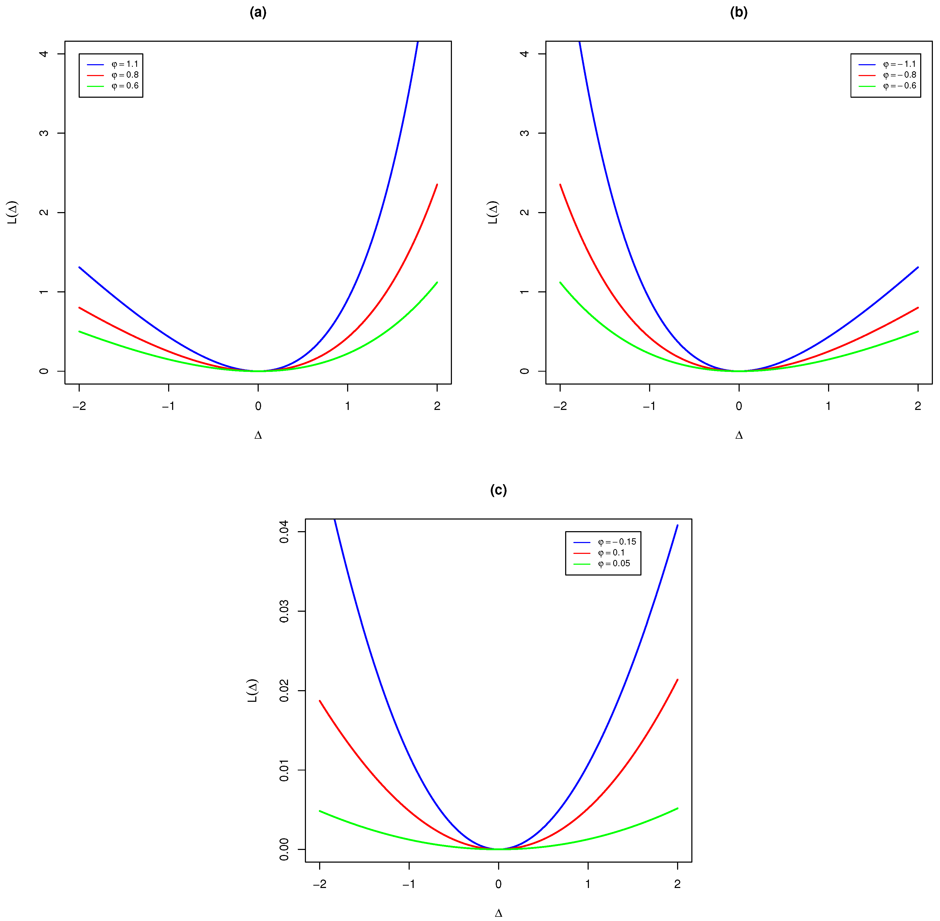
From (1), the sign and magnitude of the shape parameter $\phi$ represent the direction and degree of symmetry of LINEX loss. Several comments are necessary regarding (1). First, for $\phi >0$, overestimation is more serious than underestimation, and vice versa. When $\phi$ is close to zero, the LINEX loss is approximately the squared error loss and therefore almost symmetric. For clarity of illustration, various plots of the LINEX loss function $L(\Delta )$ with $\Delta =\tilde{\theta }-\theta$ are presented in Figure 1 under different choices of parameter $\phi$. The plots also demonstrate that positive, negative and small values of $\phi$ give more weight for overestimating, underestimating and almost equal estimation, respectively. It is observed from Figure 1a that, for positive values of $\phi$, the function is completely asymmetric, with overestimation being more harmful than underestimation. For negative values of $\phi$, as in Figure 1b, the function grows approximately exponentially when $\Delta <0$ and almost linearly when $\Delta >0$. Moreover, when $\phi$ tends towards zero, as in Figure 1c, the function is approximately symmetric as the squared error loss function.

Let $g\left(\theta \right|data)$ be the posterior distribution of the parameter $\theta$; then, the Bayesian estimator of $\theta$ using the LINEX loss function, denoted by ${\tilde{\theta }}^{BL}$, is given by

$${\tilde{\theta }}^{BL}=-\frac{1}{\phi }\left\{log\left[E_{\theta }\left(e^{-\phi \theta }\right)\right]\right\},\phi \ne 0,$$

(2)

where $E_{\theta }[·]$ is the expectation with respect to $g\left(\theta \right|data)$.

Due to the practicality of the asymmetric LINEX loss in many applications, including reliability, economic and social studies, among others, many authors have studied the Bayesian inference and decision analysis problems using the LINEX loss function. Dey et al. [8] explored the robustness properties of classes of LINEX losses under exponential and discrete power series families of distributions. Soliman [9] compared the Bayesian estimators of the parameters and reliability characteristics for Rayleigh distribution using quadratic and LINEX loss functions. Misra and Meulen [10] investigated the estimation of the mean of two normal populations with unknown means and common known variance using the LINEX loss function. Micheas [11] investigated robustness to loss functions employing the LINEX loss function and applied the methods to standard examples. Hoque et al. [12] analyzed the performance of the unrestricted estimator and preliminary test estimator of the linear regression model based on the LINEX loss function. Kazmi et al. [13] studied the properties of Bayesian estimators of the parameter of a class of lifetime distributions, employing various loss functions, including the LINEX loss, through simulation and real data. Theoretical results were obtained for various lifetime distributions under different data types by many authors; see, for example, the works of Pandey et al. [14], Jaheen [15], Azimi et al. [16], Ahmed [17,18], Ashour and Nassar [19], Nassar et al. [20], Kotb and Raqab [21], Chen and Gui [22] and Nassar et al. [23], among others. From practical perspectives, due to its flexibility of measuring the overestimation and underestimation and its more appropriate data fitting feature in data analysis, the LINEX loss is also widely used in many practical discussions. For instance, in order to estimate the mean of the selected normal population from two normal populations with unknown means and common known variance, Misra and Meulen [10] proposed some admissibility results for a subclass of equivalent estimators, and a sufficient condition for the inadmissibility of an arbitrary equivalent estimator was also provided. In the classical Taguchi quality model, Chang and Hung [2] used the LINEX loss to measure the loss of quality to determine optimum process parameters for the product quality. By inheriting the asymmetric merit of LINEX loss, Tang et al. [24] proposed a general multi-view LINEX SVM framework to improve the performance of multi-view learning. Estimation of the costs of non-conforming products is one of the most important inputs in the economic design of control charts. Abolmohammadi et al. [25] proposed an extending control chart by considering the LINEX loss on the basis of the Markov chain approach, and the results showed that the practical VSIX control chart based on the LINEX loss was more efficient in terms of the expected cost per hour. However, it should be mentioned here that, after extensive documentation retrieval, the statistical inferential results were obtained under LINEX loss with fixed parameter $\phi$, where a random chosen positive or negative $\phi$ was taken for indicating overestimation and underestimation, respectively, but there was no discussion on how to choose a proper value for the LINEX parameter $\phi$.

In the practical Bayesian inferential approach, with respect to LINEX loss and even other asymmetric losses, it is an inevitable challenge issue to choose the values of the LINEX parameter in practice. To balance the overestimation and underestimation for practical data analysis and to give relatively explicit weights between over- and underestimation, the value(s) of the LINEX parameter $\phi$ are usually determined through historical information, expert experience, as well as some other strategies. Obviously, inference using a fixed parametrization has limitations and the randomly given value of the parameter $\phi$ merely provides overestimation or underestimation in general and cannot provide a proper balance between overestimation and underestimation in practice. To overcome this drawback, it is more reasonable to take the idea that there are many values of the parameter $\phi$ in a given issue, and these potential values feature different weights. Therefore, it is assumed that the LINEX parameter $\phi$ is a random variable. In Bayesian inference, the main advantage of such an assumption is that, if the number of choices for the parameter $\phi$ is sufficient, the subjective prefixed value of parameter $\phi$ can be viewed as a good choice in analysis. However, within the extensive literature research and empirical illustrations, such an arbitrary subjective approach may lead to poor inferential results if there is not enough information available. The value of the parameter $\phi$ is given randomly in many practical studies, and the final “proper value” may be determined by empirical comparison and cross-validation approaches. Therefore, compared with the conventional subjective procedure, it is necessary and important to adopt an alternative method for the determination of the parameter $\phi$, where relatively objective value(s) of $\phi$ will provide a more effective balance between overestimation and underestimation in Bayesian inference. It should be mentioned here that, from the perspective of physical application, for complex macroscopical or microcosmic systems, the system has multiple normal states in its operating cycle, and the observed condition is the superposition across different detailed state combinations. Therefore, the presented approach may have potential benefits in studies of statistical physics.

Motivated by such reasons, the main aim of this paper is to introduce an alternative Bayesian analysis for parameter estimation with respect to the LINEX loss function. To overcome the subjective method for the choice of the parameter $\phi$, it is assumed that the parameter $\phi$ is denoted by a random variable with a proper probability distribution. By taking the expectation of the Bayesian estimator using the usual LINEX loss function over the distribution of $\phi$, the proposed Bayesian estimator can be obtained in consequence. The new Bayesian estimator is called the Bayesian estimator using the expected LINEX loss function. When the lifetime data come from an exponential distribution, Bayesian estimation using the expected LINEX loss is discussed and empirical illustrations are carried out to show the associated effect in the estimator(s) behavior compared with some arbitrary considered value(s) of the parameter $\phi$.

The concept of the loss (or cost) function is employed in different optimization procedures in statistical theory and the decision-making process to scheme an event in a real number and the associated loss or cost. An optimization problem always aims to minimize a loss function. As shown by the empirical results in Section 4 and Section 5, the expected LINEX loss function provides Bayesian estimators with minimum loss as measured through the Bayes risks. Therefore, we can conclude that the Bayesian estimators obtained based on the suggested technique are good estimators and can be used effectively in various fields, including reliability analysis, estimation processes, financial investment, forecasting and decision-making processes.

The rest of this paper is organized as follows. The expected LINEX and model description are discussed in Section 2. In Section 3, we obtain the Bayesian estimator of the exponential distribution using the expected LINEX loss function as well as the Bayes risk. Extensive simulation studies are presented in Section 4. Section 5 demonstrates the usefulness of the new estimators by analyzing three real data sets. Finally, the paper is concluded in Section 6.

2. Expected LINEX and Model Description

Let $\pi \left(\phi \right)$ be the probability density function (PDF) of $\phi$ with range $(-\infty ,\infty )$; then, from (2), one can obtain the Bayesian estimator of the unknown parameter $\theta$ using the expected LINEX loss function as follows:

$$\begin{array}{c}\hfill {\tilde{\theta }}^{BEL}={\int }_{-\infty }^{\infty }{\tilde{\theta }}^{BL}\left(\phi \right)\pi \left(\phi \right)d\phi ,\end{array}$$

(3)

where ${\tilde{\theta }}^{BL}\left(\phi \right)\equiv {\tilde{\theta }}^{BL}$ is the Bayesian estimator of the unknown parameter $\theta$ given by (2). One can choose a proper probability model $\pi \left(\phi \right)$ to reflect being symmetric, positive or negatively skewed, which will, in turn, give proper weights to balance overestimation and underestimation. It is noted that, compared with the conventional prefixed choice of the parameter $\phi$, the Bayesian estimation (3) under expected LINEX loss takes all possible values of the parameter $\phi$ into account, and gives different probabilistic weights to each value. Then, the overall balance between overestimation and underestimation is characterized by the weighted sum in the full range $(-\infty ,\infty )$ of the parameter $\phi$, which may be more objective and robust than the conventional approach in Bayesian analysis.

Let X be a random variable following the exponential distribution with parameter $\beta$ with the PDF

$$\begin{array}{c}\hfill f(x;\beta )=\beta e^{-\beta x},x>0,\beta >0,\end{array}$$

(4)

where $\beta$ is the scale parameter. Suppose that $X_1,X_2,\dots ,X_n$ is a random sample of size n from the exponential distribution (4), and $x_1,x_2,\dots ,x_n$ is the associated observation of $X_1,X_2,\dots ,X_n$. Then, the likelihood function of $\beta$ can be written as

$$\begin{array}{c}\hfill L\left(\beta \right|data)={\beta }^n{e}^{-\beta {\sum }_{i=1}^n{x}_i}.\end{array}$$

(5)

By direct computation, it is known that the maximum likelihood estimator (MLE) of the parameter $\beta$ is

$$\begin{array}{c}\hfill \widehat{\beta }=\frac{n}{{\sum }_{i=1}^n{x}_i}.\end{array}$$

(6)

To obtain the Bayesian estimator of the parameter $\beta$, we need to determine the prior distribution, say $g\left(\beta \right)$, of $\beta$. In this paper, a conjugate prior distribution of $\beta$ is used as the gamma distribution with density function

$$\begin{array}{c}\hfill \pi \left(\beta \right)\propto {\beta }^{a-1}{e}^{-b\beta },\beta >0.\end{array}$$

(7)

It is seen that the prior distribution in (7) is a natural conjugate prior because it generates a posterior distribution that relates to the same family. Furthermore, the posterior distribution generated from the natural conjugate prior can be easily mathematically manipulated. The researcher can select the values of the hyper-parameters a and b to accommodate the prior knowledge. Moreover, the Jeffreys prior can be derived as a special case of (7) by replacing $a=b=0$; for more details, see Kundu and Howlader [26]. Then, the posterior distribution of $\beta$ is given by

$$\begin{array}{c}\hfill g\left(\beta \right|data)\propto {\beta }^{n+a-1}{e}^{-\beta \left(b+{\sum }_{i=1}^n{x}_i\right)}.\end{array}$$

(8)

Under the symmetric squared error (SE) loss function, the Bayesian estimator of $\beta$ is the posterior mean, i.e.,

$$\begin{array}{c}\hfill {\tilde{\beta }}^{BS}=\frac{n+a}{b+{\sum }_{i=1}^n{x}_i}.\end{array}$$

(9)

Similarly, the Bayesian estimator of $\beta$ using the LINEX loss function can be written from (2) as

$$\begin{array}{c}\hfill {\tilde{\beta }}^{BL}=\frac{n+a}{\phi }log\left(1+\frac{\phi }{b+{\sum }_{i=1}^n{x}_i}\right).\end{array}$$

(10)

Further, to obtain the Bayesian estimator of $\beta$ using the expected LINEX loss function, we propose the following three probabilistic distributions for the parameter $\phi \in (-\infty ,\infty )$ as

$$\begin{gathered} {\pi }_1\left(\phi \right)=\frac{c{e}^{-\phi }}{{\left(1+e^{-\phi }\right)}^{c+1}},c>0, \\ {\pi }_2\left(\phi \right)=\frac{1}{\sqrt{2\pi }}{e}^{-\frac{{(\phi -\mu )}^2}{2}},-\infty <\mu <\infty , \\ {\pi }_3\left(\phi \right)=exp\left(-e^{-\left(\phi -d\right)}-\phi +d\right),-\infty <d<\infty . \end{gathered}$$

(11)

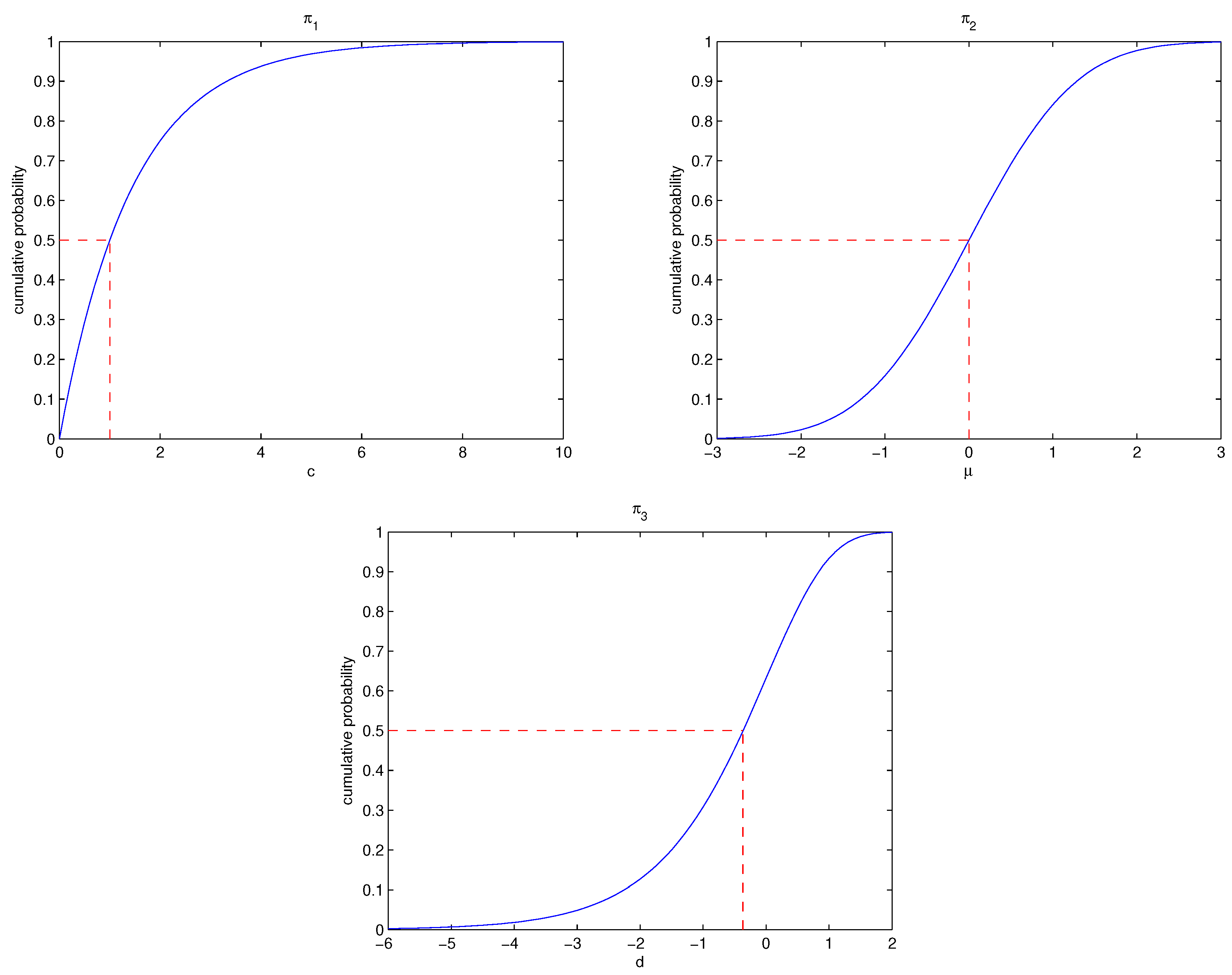
From (11), it is noted that ${\pi }_1\left(\phi \right)$ is the generalized logistic type-I (this type has also been called the “skew-logistic”) distribution with shape parameter c, ${\pi }_2\left(\phi \right)$ is the normal distribution with scale parameter 1 and location parameter $\mu$, and ${\pi }_3\left(\phi \right)$ is the standard Gumbel or extreme value distribution with location parameter d. It is seen that, in different distributions ${\pi }_1\left(\phi \right),{\pi }_2\left(\phi \right)$ and ${\pi }_3\left(\phi \right)$, the parameter $\phi$ features different probability weights at different values in full range $(-\infty ,\infty )$, and that overestimation and underestimation could be well modeled by choosing constants $c,\mu$ and d properly. For illustration, the cumulative probability weight for the parameter $\phi$ is calculated and the associated plots are presented in Figure 2 with a change in parameters $c,\mu$ and d, respectively. One could see that when parameters $c>1$ $\mu >0$ and $d>-0.36651$, the weights of overestimation are more serious than underestimation using distributions ${\pi }_1\left(\phi \right)$, ${\pi }_2\left(\phi \right)$ and ${\pi }_3\left(\phi \right)$, respectively. The distributions in (11) will be used to obtain the Bayesian estimator of the parameter $\beta$ using the expected LINEX loss function in the next section.

Remark 1.

It should be mentioned here that the choice of the distribution for the parameter φ is a tricky issue in practice. The main principle is that the model of φ should be a distribution with full range $(-\infty ,\infty )$. On this basis, due to historical information and expert experience, among others, if there are sufficient extra data used regarding φ, one could use a goodness-of-fit technique to find a proper model from among different candidates, whereas, if there is scarce information about φ’s distributional characteristics, one could use a skewed distribution with concise expression from an ease of computation perspective. Further, one could also refer to the maximum likelihood and moment methods to give proper estimates for parameters $c,\mu$ and d, respectively, by using the information of φ in consequence.

Remark 2.

A proper probability model $\pi \left(\varphi \right)$ provides weights to balance between overestimation and underestimation compared with fixed ϕ. In general, when the random model $\pi \left(\varphi \right)$ is available, the optimal Bayesian estimator of θ from a decision-making perspective can be obtained as follows:

$$\begin{array}{c}\hfill \tilde{\theta }=\underset{\delta }{min}\left\{E_{\theta }{E}_{\varphi }L(\theta ,\delta )\right\},\end{array}$$

where $L(·,·)$ is the loss function, δ is the estimator of parameter θ, $E_{\theta }(·)$ denotes the expectation with the posterior distribution of θ, and $E_{\varphi }$ denotes the expectation with the random model of ϕ. Under this approach, it is clear that the proposed expected Bayesian estimator can be viewed as the mixture of conventional Bayesian estimation under the weight $\pi \left(\varphi \right)$ at each value of ϕ, and that the estimator refers to (3) under the expected LINEX loss from the decision-making procedure.

3. Bayesian Estimation Using Expected LINEX

In this section, the alternative Bayesian estimators of the exponential parameter $\beta$ are proposed under the expected LINEX approach with the different probability distributions in (11), respectively. In addition, in order to investigate the behavior of the different estimators, the Bayesian risks are also presented in this section.

3.1. Bayesian Estimation Using Expected LINEX

Using the following series (e.g., formula 1.511 of Gradshteyn and Ryzhik [27]),

$$\begin{array}{c}\hfill log(1+z)=\sum _{j=1}^{\infty }\frac{{(-1)}^{j+1}{z}^j}{j},\left|z\right|<1,\end{array}$$

the ${\tilde{\beta }}^{BL}$ in (10) with respect to the LINEX loss function can be rewritten as

$$\begin{array}{c}\hfill {\tilde{\beta }}^{BL}=(n+a)\sum _{j=1}^{\infty }{v}_j{\phi }^{j-1}\mathrm{with}{v}_j=\frac{{(-1)}^{j+1}}{j{\left(b+{\sum }_{i=1}^n{x}_i\right)}^j}.\end{array}$$

(12)

From (3), (11) and (12), the Bayesian estimator ${\tilde{\beta }}_1^{BEL}$ of the parameter $\beta$ using the expected LINEX loss with respect to ${\pi }_1\left(\phi \right)$ can be obtained as follows:

$$\begin{array}{cc}\hfill {\tilde{\beta }}_1^{BEL}& =(n+a)\sum _{j=1}^{\infty }{v}_j{\int }_{-\infty }^{\infty }{\phi }^{j-1}\frac{c{e}^{-\phi }}{{\left(1+e^{-\phi }\right)}^{c+1}}d\phi .\hfill \end{array}$$

(13)

We use the generalized Hurwitz–Lerch Zeta function introduced by Goyal and Laddha [28], defined by

$$\begin{array}{ccc}\hfill {\psi }_M^{*}(u,v,r)& =& \frac{1}{\Gamma \left(v\right)}{\int }_0^{\infty }{t}^{v-1}\frac{e^{-rt}}{{\left(1-u{e}^{-t}\right)}^M}dt\hfill \\ & =& \sum _{k=0}^{\infty }\frac{{\left(M\right)}_k{u}^k}{{(r+k)}^{v}k!},\hfill \end{array}$$

(14)

where $M\in \mathbb{C}$, $r\in \mathbb{C}\setminus {\mathbb{Z}}_0^{-}$, $\left|u\right|<1$, $\mathfrak{R}\{v-M\}>1$ and ${\left(M\right)}_k=\frac{\Gamma (M+k)}{\Gamma \left(M\right)}$ denotes the Pochhammer symbol, with the convention ${\left(M\right)}_0=1$; see Srivastava et al. [29]. Hence, the Bayes estimator ${\tilde{\beta }}_1^{BEL}$ takes the form

$$\begin{array}{cc}\hfill {\tilde{\beta }}_1^{BEL}& =c(n+a)\sum _{j=1}^{\infty }{v}_j\Gamma \left(j\right)\left\{{\psi }_{c+1}^{*}(-1,j,1)+{(-1)}^{j-1}{\psi }_{c+1}^{*}(-1,j,c)\right\},j>c.\hfill \end{array}$$

(15)

Following the same approach, the Bayesian estimator ${\tilde{\beta }}_2^{BEL}$ of the parameter $\beta$ using the expected LINEX loss with respect to ${\pi }_2\left(\phi \right)$ is given by

$$\begin{array}{cc}\hfill {\tilde{\beta }}_2^{BEL}& =(n+a)\sum _{j=1}^{\infty }{v}_j{\int }_{-\infty }^{\infty }{\phi }^{j-1}\frac{1}{\sqrt{2\pi }}{e}^{-\frac{{(\phi -\mu )}^2}{2}}d\phi \hfill \\ \hfill & =\frac{(n+a)e^{-\frac{{\mu }^2}{2}}}{\sqrt{2\pi }}\sum _{j=1}^{\infty }{v}_j{\int }_{-\infty }^{\infty }{\phi }^{j-1}{e}^{-\frac{{\phi }^2}{2}+\mu \phi }d\phi \hfill \\ \hfill & =(n+a)e^{-\frac{3}{4}{\mu }^2}\sum _{j=1}^{\infty }{v}_j{e}^{\frac{\pi }{2}(j-1)}{D}_{j-1}\left(\mu \right),\hfill \end{array}$$

(16)

where, $D_u\left(y\right)$ is the parabolic cylinder function (see Gradshteyn and Ryzhik [27], formula 9.24(0,1), page 1028).

Further, the Bayesian estimator ${\tilde{\beta }}_3^{BEL}$ of the parameter $\beta$ using ${\pi }_3\left(\phi \right)$ under the expected LINEX loss can be expressed as

$$\begin{array}{cc}\hfill {\tilde{\beta }}_3^{BEL}& =(n+a)\sum _{j=1}^{\infty }{v}_j{\int }_{-\infty }^{\infty }{\phi }^{j-1}exp\left(-e^{-\left(\phi -d\right)}-\phi +d\right)d\phi \hfill \\ \hfill & =(n+a)\sum _{j=1}^{\infty }{v}_j{\int }_0^{\infty }{\left(d-log\left(y\right)\right)}^{j-1}{e}^{-y}dy,(\mathrm{with}y=e^{-\phi +d}).\hfill \end{array}$$

(17)

Using the binomial expansion for ${\left(u+v\right)}^m={\sum }_{n=0}^m\left(\genfrac{}{}{0pt}{}{m}{n}\right)u^{m-n}{v}^n$ in the last integral (17), one further has

$$\begin{array}{c}\hfill {\tilde{\beta }}_3^{BEL}=(n+a)\sum _{j=1}^{\infty }\sum _{m=0}^{j-1}{(-1)}^m\left(\genfrac{}{}{0pt}{}{j-1}{m}\right)v_j{d}^{j-m-1}{\int }_0^{\infty }{\left(log\left(y\right)\right)}^m{e}^{-y}dy,\end{array}$$

(18)

Using the result by Nadarajah [30],

$$\begin{array}{ccc}\hfill I(m,\omega )& =& {\int }_0^{\infty }{[log\left(y\right)]}^m{e}^{-y(\omega +1)}dy\hfill \\ & =& {\left(\frac{\partial }{\partial s}\right)}^m\left[{(\omega +1)}^{-s}\Gamma \left(s\right)\right]{\mid }_{s=1}.\hfill \end{array}$$

(19)

Then, by combining (18) and (19), the estimator ${\tilde{\beta }}_3^{BEL}$ reduces to

$$\begin{array}{c}\hfill {\tilde{\beta }}_3^{BEL}=(n+a)\sum _{j=1}^{\infty }\sum _{m=0}^{j-1}{(-1)}^m\left(\genfrac{}{}{0pt}{}{j-1}{m}\right)v_j{d}^{j-m-1}{\left(\frac{\partial }{\partial s}\right)}^m\Gamma \left(s\right){\mid }_{s=1}.\end{array}$$

(20)

Clearly, the Monte Carlo integration technique can be used to approximate the Bayesian estimators (15), (16) and (20) of the parameter $\beta$ under the expected LINEX loss with respect to the different probability distributions in (11). In this case, we can obtain ${\tilde{\beta }}_k^{BEL},k=1,2,3$ based on ${\tilde{\beta }}^{BL}$ in (10) as follows:

$$\begin{array}{ccc}\hfill {\tilde{\beta }}_k^{BEL}& \approx & \frac{n+a}{N}\sum _{t=1}^N{y}_{kt}^{-1}log\left(1+\frac{y_{kt}}{b+{\sum }_{i=1}^n{x}_i}\right),k=1,2,3,\hfill \end{array}$$

where $y_{k1},\dots ,y_{kN}$ are the generated random numbers from ${\pi }_k\left(\phi \right),k=1,2,3$, respectively.

3.2. Bayes Risks

In order to compare the behavior of different Bayesian estimators using the expected LINEX loss function, the Bayes risks are also provided in this section. We denote by $\tilde{\beta }$ the estimator of $\beta$, and then the associated Bayes risk of $\tilde{\beta }$ is defined as $E_{\beta }\left[L(\tilde{\beta },\beta )\right]$, where $L(\tilde{\beta },\beta )$ is any loss function and the expectation is taken over the posterior distribution of $\beta$. Therefore, the Bayes risk using the LINEX loss function can be obtained from (1) and (8) as

$$\begin{array}{cc}\hfill B{R}^L& ={\int }_0^{\infty }\left[e^{\phi ({\tilde{\beta }}^{BL}-\beta )}-\phi ({\tilde{\beta }}^{BL}-\beta )-1\right]{\beta }^{n+a-1}{e}^{-\beta \left(b+{\sum }_{i=1}^n{x}_i\right)}d\beta \hfill \\ \hfill & =\phi \left[\frac{n+a}{b+{\sum }_{i=1}^n{x}_i}-\frac{n+a}{\phi }log\left(1+\frac{\phi }{b+{\sum }_{i=1}^n{x}_i}\right)\right].\hfill \end{array}$$

(21)

Correspondingly, the Bayes risk using the expected LINEX loss function can be defined as follows:

$$\begin{array}{cc}\hfill B{R}^{EL}& ={\int }_{-\infty }^{\infty }B{R}^L\left(\phi \right)\pi \left(\phi \right)d\phi ,\hfill \end{array}$$

(22)

where $B{R}^L\left(\phi \right)\equiv B{R}^L$. Therefore, from (11) and (22), the Bayes risk of ${\tilde{\beta }}_1^{BEL}$ using the expected LINEX loss function with respect to ${\pi }_1\left(\phi \right)$ can be expressed as

$$\begin{array}{cc}\hfill B{R}_1^{EL}& ={\int }_{-\infty }^{\infty }\phi \left\{\frac{n+a}{b+{\sum }_{i=1}^n{x}_i}-\frac{n+a}{\phi }log\left(1+\frac{\phi }{b+{\sum }_{i=1}^n{x}_i}\right)\right\}\frac{c{e}^{-\phi }}{{\left(1+e^{-\phi }\right)}^{c+1}}d\phi \hfill \\ \hfill & ={\int }_{-\infty }^{\infty }\phi \left\{\frac{n+a}{b+{\sum }_{i=1}^n{x}_i}-(n+a)\sum _{j=1}^{\infty }{v}_j{\phi }^{j-1}\right\}\frac{c{e}^{-\phi }}{{\left(1+e^{-\phi }\right)}^{c+1}}d\phi \hfill \\ \hfill & =\frac{c(n+a)}{b+{\sum }_{i=1}^n{x}_i}\left\{{\psi }_{c+1}^{*}(-1,2,1)-{\psi }_{c+1}^{*}(-1,2,c)\right\}\hfill \\ \hfill & -c(n+a)\sum _{j=1}^{\infty }{v}_j\Gamma (j+1)\left\{{\psi }_{c+1}^{*}(-1,j+1,1)+{(-1)}^j{\psi }_{c+1}^{*}(-1,j+1,c)\right\},j>c-1.\hfill \end{array}$$

(23)

Similarly, using ${\pi }_2\left(\phi \right)$ in (11) and (22), the Bayes risk of ${\tilde{\beta }}_2^{BEL}$ using the expected LINEX loss function can be obtained as

$$\begin{array}{cc}\hfill B{R}_2^{EL}& ={\int }_{-\infty }^{\infty }\phi \left\{\frac{n+a}{b+{\sum }_{i=1}^n{x}_i}-\frac{n+a}{\phi }log\left(1+\frac{\phi }{b+{\sum }_{i=1}^n{x}_i}\right)\right\}\frac{1}{\sqrt{2\pi }}{e}^{-\frac{{(\phi -\mu )}^2}{2}}d\phi \hfill \\ \hfill & ={\int }_{-\infty }^{\infty }\phi \left\{\frac{n+a}{b+{\sum }_{i=1}^n{x}_i}-(n+a)\sum _{j=1}^{\infty }{v}_j{\phi }^{j-1}\right\}\frac{1}{\sqrt{2\pi }}{e}^{-\frac{{(\phi -\mu )}^2}{2}}d\phi \hfill \\ \hfill & =\frac{\mu (n+a)}{b+{\sum }_{i=1}^n{x}_i}-(n+a)e^{-\frac{3}{4}{\mu }^2}\sum _{j=1}^{\infty }{v}_j{e}^{\frac{\pi }{2}j}{D}_j\left(\mu \right).\hfill \end{array}$$

(24)

Finally, the Bayes risk of ${\tilde{\beta }}_3^{BEL}$ using the expected LINEX loss function based on ${\pi }_3\left(\phi \right)$ can be expressed as

$$\begin{array}{cc}\hfill B{R}_3^{EL}& ={\int }_{-\infty }^{\infty }\phi \left\{\frac{n+a}{b+{\sum }_{i=1}^n{x}_i}-(n+a)\sum _{j=1}^{\infty }{v}_j{\phi }^{j-1}\right\}{e}^{\left(-e^{-\left(\phi -d\right)}-\phi +d\right)}d\phi \hfill \\ \hfill & =\frac{(n+a)\left(d+\gamma \right)}{b+{\sum }_{i=1}^n{x}_i}-(n+a)\sum _{j=1}^{\infty }\sum _{m=0}^{j-1}{(-1)}^m\left(\genfrac{}{}{0pt}{}{j-1}{m}\right)v_j{d}^{j-m-1}{\left(\frac{\partial }{\partial s}\right)}^m{\Gamma \left(s\right)|}_{s=1},\hfill \end{array}$$

(25)

where $\gamma \simeq 0.5772156649\dots$ is known as Euler’s constant.

Another simple way to obtain the Bayes risk of ${\tilde{\beta }}_k^{BEL},k=1,2,3$ is to use the Monte Carlo integration routine. In this case, we have from (22) the following:

$$\begin{array}{ccc}\hfill B{R}_k^{EL}& \approx & \frac{1}{N}\sum _{t=1}^N\left[\frac{y_{kt}(n+a)}{b+{\sum }_{i=1}^n{x}_i}-(n+a)log\left(1+\frac{y_{kt}}{b+{\sum }_{i=1}^n{x}_i}\right)\right],k=1,2,3,\hfill \end{array}$$

where $y_{k1},\dots ,y_{kN}$ are the generated random numbers from ${\pi }_k\left(\phi \right),k=1,2,3$, respectively.

4. Simulation Study

In this section, in order to investigate and compare the performance of different Bayesian estimators using the expected LINEX loss function, along with those based on SE and LINEX loss functions, extensive Monte Carlo simulations are carried out for illustration. The simulation procedure can be described by the following steps.

Step 1

Determine the value of the parameter $\beta$ and the sample size n.

Step 2

Generate a random sample from the exponential distribution, where $x_i=-\frac{log(1-u_i)}{\beta }$, $i=1,\dots ,n$ where $U\sim uniform(0,1)$.

Step 3

For given values of gamma hyper-parameters a and b, generate $\beta$ from the gamma prior density (7).

Step 4

The Bayesian estimates ${\tilde{\beta }}^{BS},{\tilde{\beta }}^{BL}$ and the associated Bayesian estimates ${\tilde{\beta }}_1^{BEL},{\tilde{\beta }}_2^{BEL},{\tilde{\beta }}_3^{BEL}$ using the expected LINEX loss of the parameter $\beta$ are computed.

Step 5

Based on multiple replications, the performance of the different Bayesian estimates is evaluated in terms of criteria quantities of the mean relative estimate (MRE) and mean square error (MSE) as well as the Bayes risks.

In this procedure, the simulation is performed by considering different values of $\beta =0.5,2$ and sample sizes $n=20,40,60,80,100$, respectively. Meanwhile, the gamma hyper-parameters are chosen in such a way that the prior mean becomes the expected value of the corresponding parameters. We assume $a=1,b=2$ for $\beta =0.5$ and $a=2,b=1$ for $\beta =2$ in this simulation. Further, the Bayesian estimates with respect to the LINEX loss function are calculated with selected $\phi =1.5$ in all the settings, whereas the Bayesian estimates using the expected LINEX loss function are obtained under different parameter values $c,\mu$ and d of distributions ${\pi }_j\left(\phi \right),j=1,2,3$, respectively. For each ${\pi }_j\left(\phi \right)$, five configurations (Conf) are proposed, as shown in

Table 1. Selected parameter values of ${\pi }_j\left(\phi \right),j=1,2,3$.

Distribution	Parameter	Conf
		1	2	3	4	5
${\pi }_1\left(\phi \right)$	c	0.2	0.5	1	2	5
${\pi }_2\left(\phi \right)$	$\mu$	−2	−0.5	0	2	5
${\pi }_3\left(\phi \right)$	d	−2	−0.5	0	2	5

. As mentioned before, when $c>1$$\mu >0$ and $d>-0.36651$, the weights of overestimation are more serious than underestimation employing the distributions ${\pi }_1\left(\phi \right)$, ${\pi }_2\left(\phi \right)$ and ${\pi }_3\left(\phi \right)$, respectively. Therefore, the values in Table 1 are selected to reflect the impact of these parameters on the performance of the different estimates using the expected LINEX loss function. Based on 1000 replications, the criteria quantities MRE, MSE and the Bayes risks are displayed in

Table 2. The MREs of the different estimators for $\beta =0.5$ and 2.

Method	Conf	$\mathit{n}=20$	$\mathit{n}=40$	$\mathit{n}=60$	$\mathit{n}=80$	$\mathit{n}=100$
$\beta =0.5$
${\tilde{\beta }}^{BS}$	-	1.0423	1.0218	1.0083	1.0132	1.0087
${\tilde{\beta }}^{BL}$	-	1.0225	1.0121	1.0020	1.0084	1.0050
${\tilde{\beta }}_1^{BEL}$	1	1.1121	1.0472	1.0218	1.0215	1.0138
	2	1.0634	1.0313	1.0144	1.0178	1.0123
	3	1.0431	1.0220	1.0084	1.0133	1.0088
	4	1.0295	1.0154	1.0041	1.0101	1.0062
	5	1.0155	1.0085	0.9996	1.0066	1.0035
${\tilde{\beta }}_2^{BEL}$	1	1.0707	1.0351	1.0169	1.0197	1.0139
	2	1.0494	1.0251	1.0104	1.0148	1.0100
	3	1.0464	1.0189	1.0149	1.0118	1.0044
	4	1.0164	1.0090	0.9999	1.0069	1.0037
	5	0.9803	0.9906	0.9877	0.9975	0.9963
${\tilde{\beta }}_3^{BEL}$	1	1.0625	1.0313	1.0144	1.0178	1.0124
	2	1.0416	1.0214	1.0080	1.0130	1.0086
	3	1.0387	1.0152	1.0124	1.0100	1.0029
	4	1.0093	1.0054	0.9976	1.0051	1.0023
	5	0.9739	0.9871	0.9854	0.9958	0.9948
$\beta =2$
${\tilde{\beta }}^{BS}$	-	1.0410	1.0224	1.0178	1.0099	1.0090
${\tilde{\beta }}^{BL}$	-	0.9710	0.9860	0.9932	0.9915	0.9942
${\tilde{\beta }}_1^{BEL}$	1	1.1452	0.9712	0.9331	0.9109	0.9019
	2	1.1421	1.0567	1.0363	1.0212	1.0165
	3	1.0535	1.0252	1.0190	1.0105	1.0094
	4	0.9995	0.9994	1.0019	0.9979	0.9993
	5	0.9518	0.9739	0.9845	0.9847	0.9886
${\tilde{\beta }}_2^{BEL}$	1	1.1669	1.0783	1.0538	1.0362	1.0299
	2	1.0716	1.0363	1.0268	1.0165	1.0142
	3	1.0402	1.0319	1.0200	1.0040	1.0099
	4	0.9528	0.9753	0.9857	0.9858	0.9895
	5	0.8477	0.9137	0.9417	0.9520	0.9619
${\tilde{\beta }}_3^{BEL}$	1	1.1299	1.0621	1.0434	1.0286	1.0239
	2	1.0422	1.0218	1.0171	1.0093	1.0085
	3	1.0129	1.0176	1.0105	0.9970	1.0041
	4	0.9305	0.9630	0.9770	0.9791	0.9841
	5	0.8197	0.9032	0.9340	0.9460	0.9569

,

Table 3. The MSEs of the different estimators for $\beta =0.5$ and 2.

Method	Conf	$\mathit{n}=20$	$\mathit{n}=40$	$\mathit{n}=60$	$\mathit{n}=80$	$\mathit{n}=100$
$\beta =0.5$
${\tilde{\beta }}^{BS}$	-	0.0132	0.0066	0.0042	0.0035	0.0023
${\tilde{\beta }}^{BL}$	-	0.0119	0.0062	0.0041	0.0034	0.0022
${\tilde{\beta }}_1^{BEL}$	1	0.0207	0.0078	0.0047	0.0037	0.0024
	2	0.0149	0.0069	0.0044	0.0036	0.0023
	3	0.0132	0.0066	0.0042	0.0035	0.0023
	4	0.0123	0.0063	0.0042	0.0034	0.0022
	5	0.0115	0.0061	0.0041	0.0033	0.0022
${\tilde{\beta }}_2^{BEL}$	1	0.0155	0.0071	0.0045	0.0036	0.0023
	2	0.0137	0.0067	0.0043	0.0035	0.0023
	3	0.0132	0.0066	0.0041	0.0031	0.0023
	4	0.0115	0.0061	0.0041	0.0033	0.0022
	5	0.0100	0.0057	0.0039	0.0032	0.0021
${\tilde{\beta }}_3^{BEL}$	1	0.0148	0.0069	0.0044	0.0036	0.0023
	2	0.0131	0.0066	0.0042	0.0035	0.0023
	3	0.0126	0.0065	0.0040	0.0031	0.0023
	4	0.0112	0.0060	0.0040	0.0033	0.0022
	5	0.0098	0.0056	0.0039	0.0032	0.0021
$\beta =2$
${\tilde{\beta }}^{BS}$	-	0.189	0.1025	10.0651	0.0465	0.0389
${\tilde{\beta }}^{BL}$	-	0.1413	0.0876	0.0580	0.0431	0.0365
${\tilde{\beta }}_1^{BEL}$	1	0.5379	0.1172	0.0793	0.0729	0.0716
	2	0.3810	0.1312	0.0754	0.0509	0.0415
	3	0.2100	0.1049	0.0658	0.0467	0.0390
	4	0.1576	0.0920	0.0600	0.9979	0.0371
	5	0.1389	0.0857	0.0569	0.0426	0.0361
${\tilde{\beta }}_2^{BEL}$	1	0.4146	0.1499	0.0853	0.0565	0.0455
	5	0.2289	0.1117	0.0691	0.0484	0.0402
	3	0.2027	0.0963	0.0663	0.0470	0.0382
	4	0.1374	0.0857	0.0569	0.0427	0.0361
	5	0.1711	0.0942	0.0603	0.0456	0.0376
${\tilde{\beta }}_3^{BEL}$	1	0.3306	0.1334	0.0784	0.0530	0.0432
	2	0.1928	0.1025	0.0649	0.0464	0.0388
	3	0.1765	0.0885	0.0628	0.0457	0.0371
	4	0.1343	0.0847	0.0563	0.0425	0.0359
	5	0.2065	0.0990	0.0627	0.0472	0.0386

and

Table 4. The Bayes risks of the different estimators for $\beta =0.5$ and 2.

Method	Conf	$\mathit{n}=20$	$\mathit{n}=40$	$\mathit{n}=60$	$\mathit{n}=80$	$\mathit{n}=100$
$\beta =0.5$
${\tilde{\beta }}^{BS}$	-	0.0135	0.0065	0.0042	0.0032	0.0025
${\tilde{\beta }}^{BL}$	-	0.0148	0.0072	0.0047	0.0036	0.0028
${\tilde{\beta }}_1^{BEL}$	1	0.4061	0.1617	0.1003	0.0745	0.0583
	2	0.0644	0.0291	0.0186	0.0140	0.0110
	3	0.0224	0.0107	0.0070	0.0053	0.0042
	4	0.0212	0.0105	0.0069	0.0052	0.0041
	5	0.0394	0.0196	0.0129	0.0098	0.0078
${\tilde{\beta }}_2^{BEL}$	1	0.0357	0.0167	0.0108	0.0081	0.0064
	2	0.0087	0.0041	0.0027	0.0020	0.0016
	3	0.0068	0.0032	0.0021	0.0016	0.0013
	4	0.0322	0.0159	0.0104	0.0079	0.0063
	5	0.1606	0.0810	0.0534	0.0408	0.0324
${\tilde{\beta }}_3^{BEL}$	1	0.0258	0.0122	0.0079	0.0059	0.0047
	2	0.0109	0.0053	0.0035	0.0026	0.0021
	3	0.0129	0.0063	0.0042	0.0031	0.0025
	4	0.0525	0.0262	0.0172	0.0131	0.0104
	5	0.1997	0.1014	0.0670	0.0512	0.0408
$\beta =2$
${\tilde{\beta }}^{BS}$	-	0.2053	0.1019	0.0679	0.0503	0.0403
${\tilde{\beta }}^{BL}$	-	0.2098	0.1092	0.0739	0.0552	0.0444
${\tilde{\beta }}_1^{BEL}$	1	3.1784	1.0846	0.6522	0.4615	0.3603
	2	1.1929	0.4569	0.2841	0.2042	0.1608
	3	0.3739	0.1701	0.1121	0.0828	0.0663
	4	0.2875	0.1526	0.1045	0.0787	0.0636
	5	0.5177	0.2808	0.1939	0.1466	0.1187
${\tilde{\beta }}_2^{BEL}$	1	0.6478	0.2826	0.1813	0.1321	0.1047
	2	0.1430	0.0669	0.0438	0.0322	0.0257
	3	0.1038	0.0519	0.0341	0.0249	0.0202
	4	0.4338	0.2331	0.1597	0.1202	0.0971
	5	1.9962	1.1251	0.7883	0.6006	0.4890
${\tilde{\beta }}_3^{BEL}$	1	0.4478	0.2019	0.1308	0.0957	0.0761
	2	0.1576	0.0802	0.0542	0.0405	0.0326
	3	0.1749	0.0940	0.0636	0.0471	0.0385
	4	0.6967	0.3748	0.2591	0.1959	0.1588
	5	2.6916	1.3873	0.9777	0.7474	0.6099

for $\beta =0.5$ and $\beta =2$, respectively.

From the listed results in Table 2, Table 3 and Table 4, it is noted that

• With the increase in sample size n, the MREs tend towards one and the criteria MSEs and Bayesian risks of both Bayesian estimates under common and expected losses decrease, which indicates the consistency of the associated estimates when the sample sizes increase;
• For a fixed sample size, the Bayesian estimates obtained under common LINEX loss have relatively smaller MSE than that from SE loss, whereas the associated Bayesian risks perform similarly under these two cases in general;
• In terms of minimum MSE, we can conclude that the Bayesian estimates using the expected LINEX loss function perform better than all other estimates for ${\pi }_3\left(\phi \right)$ with $d=5$ when $\beta =0.5$;
• The Bayesian estimates using ${\pi }_3\left(\phi \right)$ with $d=2$ have the smallest MSE among all other estimates when $\beta =2$;
• The Bayesian estimates using the expected LINEX loss function using ${\pi }_2\left(\phi \right)$ with $\mu =0$ have the minimum Bayes risk when compared with all other estimates.

It can be observed that when $\mu =0$, ${\pi }_2\left(\phi \right)$ reduces to the standard normal distribution. In this case, we can see that, although the distribution does not contain any parameter, it gives the best result based on the minimum Bayes risks in all cases. This is because, when we obtain the Bayesian estimate using the expected LINEX loss function, we take the expectation over all possible values for the parameter $\phi$. The same result can also be noted when $d=0$ in ${\pi }_3\left(\phi \right)$, where the Bayes risk obtained based on the expected LINEX loss function is smaller than that based on the common LINEX loss. Therefore, when the researcher does not have any information about the parameter $\phi$, one could take the expectation over all possible values for the parameter $\phi$ to obtain the Bayesian estimate using the expected LINEX loss.

5. Data Analysis

In this section, three real life data sets are used to show the applicability of the proposed estimators based on the expected LINEX loss function.

Example One. (Software reliability data) The first data set represents the time-between-failures (time unit in milliseconds) of software reliability. The original data were firstly presented by Lyu [31] and analyzed recently by Alotaibi et al. [32] and are also available in the reliaR package. The complete data set that is transformed from time-between-failures to failure times is presented in

Table A1. Software reliability data set.

4.79	7.45	10.22	15.76	26.10	28.59	35.52	41.49	42.66	44.36	45.53
58.27	62.96	74.70	81.63	100.71	102.06	104.83	110.79	118.36	122.73	145.03
149.40	152.80	156.85	162.20	164.97	168.60	173.82	179.95	182.72	195.72	203.93
206.06	222.26	238.27	241.25	249.99	256.17	282.57	282.62	284.11	294.45	318.86
323.46	329.11	340.30	344.67	353.94	398.56	405.70	407.51	422.36	429.93	461.47
482.62	491.46	511.83	526.64	532.23	537.13	543.06	560.75	561.60	589.96	592.09
610.75	615.65	630.52	673.74	687.92	698.15	753.05	768.25	801.06	828.22	849.97
885.02	892.27	911.90	951.69	962.59	965.04	976.98	986.92	1025.94

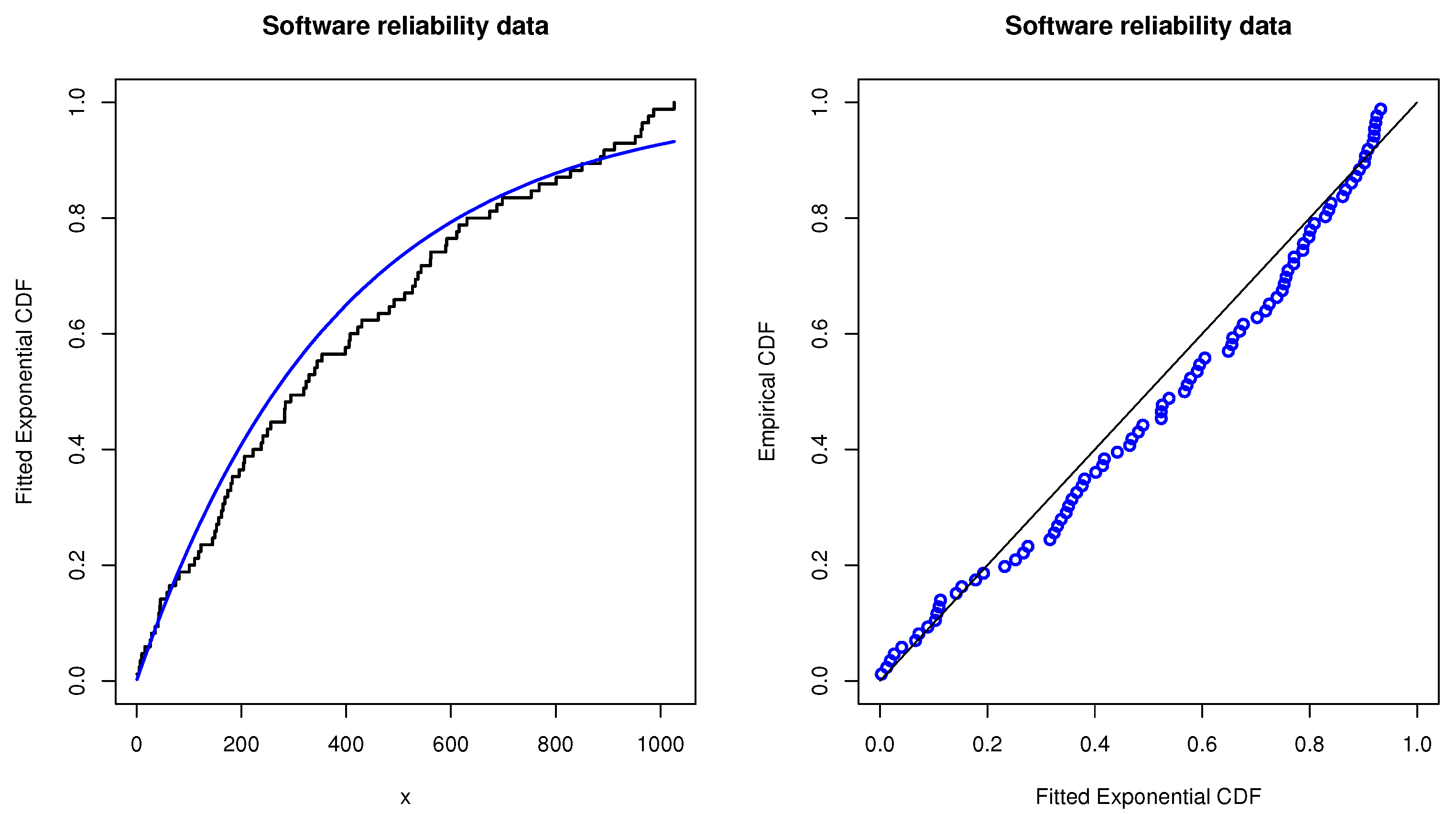
. Before proceeding further, we first check the validity of the exponential distribution to model these data by using the Kolmogorov–Smirnov (K-S) distance and the associated p-value based on the MLE of the parameter $\beta$. By direct computation, it is noted that the MLE of $\beta$ is $2.6240\times {10}^{-3}$, the K-S distance is 0.0788 and the corresponding p-value is 0.6591. Therefore, it is found that the exponential distribution could be used as an appropriate model to fit the mentioned software reliability data. For further illustration, the empirical cumulative distribution function (CDF) plot with overlaid theoretical exponential distribution and the probability–probability (P-P) plot are also shown in Figure 3 to check the goodness of fit for the software reliability data. It is also shown that the exponential distribution can be viewed as a proper model.

Based on the software reliability data set, to find the different Bayesian estimates, we select the hyper-parameters to be $a=0.011$ and $b=2.25$ in all the cases, where such choices are obtained by equating the first two moments of the gamma distribution obtained from the data with the corresponding theoretical moments. Using similarly designed scenarios given in Table 1, various Bayesian estimates are presented in

Table 5. Different estimates of $\beta$ using the software reliability data.

Method	Conf	Estimate	Bayes Risk
${\tilde{\beta }}^{BS}$	-	$2.62418\times {10}^{-3}$	$8.00631\times {10}^{-8}$
${\tilde{\beta }}^{BL}$	-	$2.62412\times {10}^{-3}$	$9.00682\times {10}^{-8}$
${\tilde{\beta }}_1^{BEL}$	1	$2.26912\times {10}^{-3}$	$6.51752\times {10}^{-7}$
	2	$2.60649\times {10}^{-3}$	$3.00326\times {10}^{-7}$
	3	$2.62394\times {10}^{-3}$	$1.31255\times {10}^{-7}$
	4	$2.62390\times {10}^{-3}$	$1.31247\times {10}^{-7}$
	5	$2.62350\times {10}^{-3}$	$2.47330\times {10}^{-7}$
${\tilde{\beta }}_2^{BEL}$	1	$2.62426\times {10}^{-3}$	$2.00169\times {10}^{-7}$
	2	$2.62420\times {10}^{-3}$	$5.00407\times {10}^{-8}$
	3	$2.62418\times {10}^{-3}$	$4.00315\times {10}^{-8}$
	4	$2.62410\times {10}^{-3}$	$2.00146\times {10}^{-7}$
	5	$2.62398\times {10}^{-3}$	$1.04071\times {10}^{-6}$
${\tilde{\beta }}_3^{BEL}$	1	$2.62423\times {10}^{-3}$	$1.46892\times {10}^{-7}$
	2	$2.62417\times {10}^{-3}$	$6.60856\times {10}^{-8}$
	3	$2.62415\times {10}^{-3}$	$7.91824\times {10}^{-8}$
	4	$2.62407\times {10}^{-3}$	$3.31714\times {10}^{-7}$
	5	$2.62395\times {10}^{-3}$	$1.31088\times {10}^{-6}$

under common SE, LINEX and the proposed expected LINEX losses, respectively. Comparing the performance of the different estimates, we can conclude that the Bayesian estimate using the expected LINEX loss function using ${\pi }_2\left(\phi \right)$ with $\mu =0$ performs better than other estimates in terms of minimum Bayes risk.

Example Two. (Breakdown of insulating fluid data) The second data set is taken from Nelson [33] and has been analyzed by many authors (see, e.g., Balakrishnan and Cramer [34], Dey and Nassar [35]). The data describe the times to breakdown of an insulating fluid subjected to a voltage of 34 kV, and the detailed lifetime data are presented in

Table A2. Breakdown of insulating fluid data set.

0.19	0.78	0.96	1.31	2.78	3.16	4.15	4.67	4.85	6.50
7.35	8.01	8.27	12.06	31.75	32.52	33.91	36.71	72.89

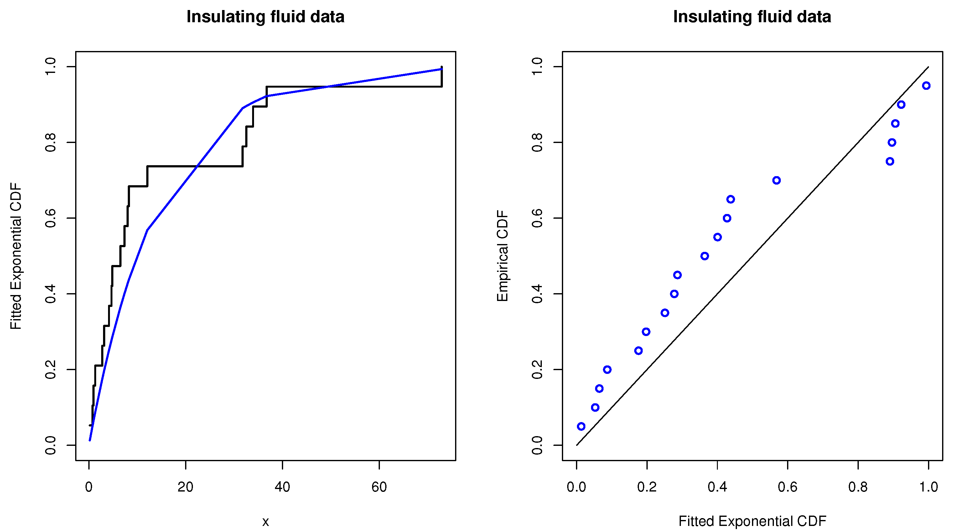
. By direct calculation, the MLE of the parameter $\beta$ for these data is $0.06964$. The K-S distance and the corresponding p-value are obtained as 0.2464 and 0.1990, respectively. Therefore, the exponential distribution is a suitable model to fit these data. For comparison, the associated empirical CDF plot with overlaid theoretical exponential distribution and the P-P plot are provided in Figure 4 as well. They also indicate that the exponential distribution is an acceptable model to fit the data.

Using the breakdown data of an insulating fluid, and following a similar approach as for example one, different Bayesian estimates are obtained under various designed scenarios. The results are presented in

Table 6. Different estimates of $\beta$ using the breakdown of insulating fluid data.

Method	Conf	Estimate	Bayes Risk
${\tilde{\beta }}^{BS}$	-	$0.07163$	$2.62502\times {10}^{-4}$
${\tilde{\beta }}^{BL}$	-	$0.07143$	$2.94237\times {10}^{-4}$
${\tilde{\beta }}_1^{BEL}$	1	$0.06229$	$2.17113\times {10}^{-3}$
	2	$0.07131$	$9.94977\times {10}^{-4}$
	3	$0.07162$	$4.30383\times {10}^{-4}$
	4	$0.07149$	$4.27258\times {10}^{-4}$
	5	$0.07134$	$8.03771\times {10}^{-4}$
${\tilde{\beta }}_2^{BEL}$	1	$0.07189$	$6.60783\times {10}^{-4}$
	2	$0.07169$	$1.64589\times {10}^{-4}$
	3	$0.07163$	$1.31254\times {10}^{-4}$
	4	$0.07136$	$6.51803\times {10}^{-4}$
	5	$0.07098$	$3.36830\times {10}^{-3}$
${\tilde{\beta }}_3^{BEL}$	1	$0.07181$	$4.84019\times {10}^{-4}$
	2	$0.07162$	$2.15802\times {10}^{-4}$
	3	$0.07155$	$2.57904\times {10}^{-4}$
	4	$0.07129$	$1.07746\times {10}^{-3}$
	5	$0.07090$	$4.23444\times {10}^{-3}$

, where the hyper-parameters are chosen as $a=0.543$ and $b=0.035$ by equating the first two moments of the gamma distribution obtained from the data with the corresponding theoretical moments. Based on the listed results in Table 6, one could also observe that the Bayesian estimate using the expected LINEX loss function using ${\pi }_2\left(\phi \right)$ with $\mu =0$ has the smallest Bayes risk among all other estimates.

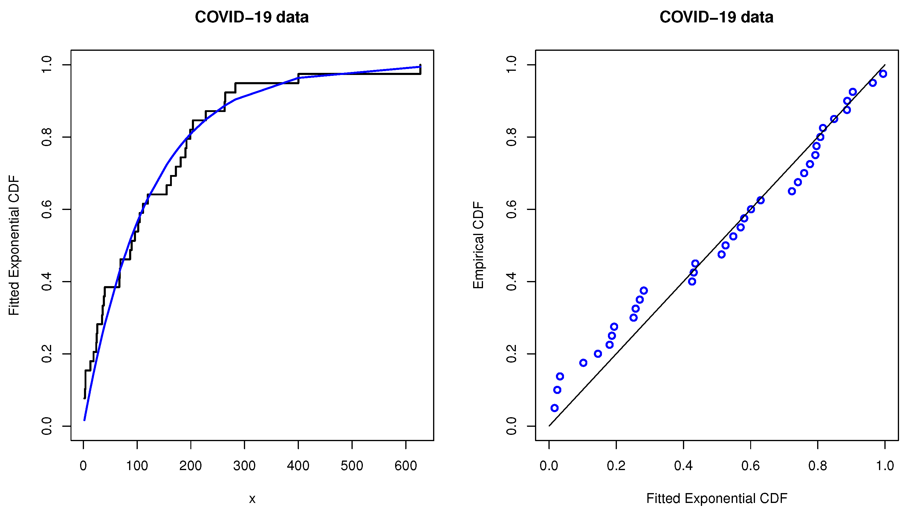
Example Three. (COVID-19 data) The third data set consists of the COVID-19 recovery cases in Pakistan from 24 March 2020 to 1 May 2020. This data set was originally analyzed by Ali et al. [36]. The complete data set is presented in

Table A3. COVID-19 data set.

13	2	2	2	3	4	26	24	25	19	4
40	87	172	38	105	155	35	264	69	283	68
199	120	67	36	102	96	90	181	190	228	111
163	204	192	627	263	400

. From the data, the MLE of $\beta$ is $0.008282$. Based on this result, the K-S distance and the corresponding p-value are 0.1213 and 0.6149, respectively. Hence, the exponential distribution is an appropriate model to fit these data. Moreover, the empirical CDF plot with overlaid theoretical exponential distribution and the P-P plot are presented in Figure 5. Figure 5 shows that the exponential distribution is an adequate model to fit the data.

To acquire the different Bayesian estimates, we set the hyper-parameter values to be $a=0.0016$ and $b=0.1230$, which are obtained by equating the first two moments of the gamma distribution got from the data with the associated theoretical moments. The different Bayesian estimates as well as the corresponding Bayes risks are tabulated in

Table 7. Different estimates of $\beta$ using COVID-19 data.

Method	Conf	Estimate	Bayes Risk
${\tilde{\beta }}^{BS}$	-	$8.28214\times {10}^{-3}$	$1.75874\times {10}^{-6}$
${\tilde{\beta }}^{BL}$	-	$8.28082\times {10}^{-3}$	$1.97817\times {10}^{-6}$
${\tilde{\beta }}_1^{BEL}$	1	$7.16357\times {10}^{-3}$	$1.43283\times {10}^{-5}$
	2	$8.22729\times {10}^{-3}$	$6.60063\times {10}^{-6}$
	3	$8.28139\times {10}^{-3}$	$2.88328\times {10}^{-6}$
	4	$8.28051\times {10}^{-3}$	$2.88206\times {10}^{-6}$
	5	$8.27843\times {10}^{-3}$	$5.43067\times {10}^{-6}$
${\tilde{\beta }}_2^{BEL}$	1	$8.28390\times {10}^{-3}$	$4.39860\times {10}^{-6}$
	2	$8.28258\times {10}^{-3}$	$1.09942\times {10}^{-6}$
	3	$8.28214\times {10}^{-3}$	$8.79372\times {10}^{-7}$
	4	$8.28038\times {10}^{-3}$	$4.39512\times {10}^{-6}$
	5	$8.27774\times {10}^{-3}$	$2.28462\times {10}^{-5}$
${\tilde{\beta }}_3^{BEL}$	1	$8.28339\times {10}^{-3}$	$3.22757\times {10}^{-6}$
	2	$8.28207\times {10}^{-3}$	$1.45140\times {10}^{-6}$
	3	$8.28163\times {10}^{-3}$	$1.73882\times {10}^{-6}$
	4	$8.27987\times {10}^{-3}$	$7.28332\times {10}^{-6}$
	5	$8.27724\times {10}^{-3}$	$2.87744\times {10}^{-5}$

. From the detailed outcomes in Table 7, one could also observe that the Bayesian estimate using the expected LINEX loss function employing ${\pi }_2\left(\phi \right)$ with $\mu =0$ has the smallest Bayes risk among all other estimates.

The simulation outcomes as well as the analysis of the three real data sets show that the performance of the Bayesian estimation using the expected LINEX loss function is superior to that of the common Bayesian approach in terms of MSE and Bayes risks. The proposed expected Bayesian estimation is a robust estimation approach that provides a weight estimation for the common Bayesian estimates. The results also show that if we select an appropriate probability distribution for $\phi$, we can reduce the MSE and Bayes risk of an estimator. The superiority of the Bayesian estimators using the expected LINEX loss function can be interpreted based on the concept of the expected value, because this estimator is obtained as the arithmetic mean of a large number of independent realizations of $\phi$. On the other hand, the usual Bayesian estimator using the LINEX loss function is obtained by choosing an arbitrary value for $\phi$. The new offered technique can be utilized significantly in different fields; for instance, one can obtain accurate estimators for some reliability indices, including reliability and hazard rate function. Moreover, in regression analysis, new estimators of the regression models can be derived using the proposed technique. Furthermore, the expected LINEX loss function can be employed in volatility forecasting.

6. Conclusions

In this paper, a new approach to obtain the Bayesian estimator using the LINEX loss function has been introduced. For avoiding the subjective choice of the LINEX parameter and giving a relatively objective balance between overestimation and underestimation, the proposed alternative method assumes that the parameter $\phi$ of the LINEX loss function has a probability distribution in the range of $(-\infty ,\infty )$. The Bayesian estimator in this case is obtained by taking the expected value of the usual Bayesian estimator using the LINEX loss function over the proposed distribution of $\phi$. When an exponential sample is available, the Bayesian estimator using the expected LINEX loss is presented for the unknown exponential parameter by considering three different distributions to the LINEX parameter $\phi$. In addition, the Bayes risks are also obtained using the different distributions. To compare the performance of the proposed Bayesian estimators with those based on the squared error and LINEX loss functions, extensive simulation studies are carried out in terms of different criteria quantities. Moreover, three real-life data sets are analyzed to show the applicability of the new method. Based on the simulation and real data analysis results, we can conclude that the Bayesian estimates using the expected LINEX loss function perform better than those based on the squared error and LINEX loss functions in terms of minimum mean square error and Bayes risk. Finally, it is of interest to employ the same approach discussed in this paper to estimate the parameters of two-parameter distributions (or more) such as Weibull and gamma distributions. This work is in progress and will be reported later.

References

1. Zellner, A. Bayesian estimation and prediction using asymmetric loss functions. J. Am. Stat. Assoc. 1986, 81, 446–451. [Google Scholar] [CrossRef]
2. Chang, Y.C.; Hung, W.L. LINEX loss functions with applications to determining the optimum process parameters. Qual. Quant. 2007, 41, 291–301. [Google Scholar] [CrossRef]
3. Khatun, N.; Matin, M.A. A Study on LINEX Loss Function with Different Estimating Methods. Open J. Stat. 2020, 10, 52. [Google Scholar] [CrossRef] [Green Version]
4. Ali, S.; Aslam, M.; Abbas, N.; Kazmi, S.M.A. Scale parameter estimation of the Laplace model using different asymmetric loss functions. Int. J. Stat. Probab. 2012, 1, 105–127. [Google Scholar] [CrossRef] [Green Version]
5. Ali, S. On the Bayesian estimation of the weighted Lindley distribution. J. Stat. Comput. Simul. 2015, 85, 855–880. [Google Scholar] [CrossRef]
6. Klebanov, L.B. Universal loss function and unbiased estimation. Dokl. Akad. Nank SSSR Soviet Math. Dokl. 1972, 203, 1249–1251. [Google Scholar]
7. Varian, H.R. A Bayesian Approach to Real Estate Assessment. In Studies in Bayesian Econometrics and Statistics: In Honor of L. J. Savage; Savage, L.J., Feinberg, S.E., Zellner, A., Eds.; North-Holland Pub. Co.: Amsterdam, The Netherlands, 1975; pp. 195–208. [Google Scholar]
8. Dey, D.; Lou, K.; Bose, S. A Bayesian approach to loss robustness. Stat. Decis. 1998, 16, 65–87. [Google Scholar] [CrossRef]
9. Soliman, A.A. Comparison of linex and quadratic bayes estimators foe the rayleigh distribution. Commun. Stat.-Theory Methods 2000, 29, 95–107. [Google Scholar] [CrossRef]
10. Misra, N.; van der Meulen, E.C. On estimating the mean of the selected normal population under the LINEX loss function. Metrika 2003, 58, 173–183. [Google Scholar] [CrossRef]
11. Micheas, A.C. A unified approach to Prior and Loss Robustness. Commun. Stat.-Theory Methods 2006, 35, 309–323. [Google Scholar] [CrossRef]
12. Hoque, Z.; Khan, S.; Wesolowski, J. Performance of preliminary test estimator under linex loss function. Commun. Stat.-Theory Methods 2009, 38, 252–261. [Google Scholar] [CrossRef] [Green Version]
13. Kazmi, S.M.A.; Aslam, M.; Ali, S. Preference of prior for the class of life-time distributions under different loss functions. Pak. J. Stat. 2012, 28, 467–487. [Google Scholar]
14. Pandey, M.; Singh, V.P.; Srivastava, C.P.L. A Bayesian estimation of reliability model using the LINEX loss function. Microelectron. Reliab. 1994, 34, 1519–1523. [Google Scholar] [CrossRef]
15. Jaheen, Z.F. A Bayesian analysis of record statistics from the Gompertz model. Appl. Math. Comput. 2003, 145, 307–320. [Google Scholar] [CrossRef]
16. Azimi, R.; Yaghmaei, F.; Azimi, D. Comparison of Bayesian estimation methods for Rayleigh progressive censored data under the different asymmetric loss function. Int. J. Appl. Math. Res. 2012, 1, 452–461. [Google Scholar] [CrossRef] [Green Version]
17. Ahmed, E.A. Bayesian estimation based on progressive Type-II censoring from two parameter bathtub-shaped lifetime model: An Markov chain Monte Carlo approach. J. Appl. Stat. 2014, 41, 752–768. [Google Scholar] [CrossRef]
18. Ahmed, E.A. Estimation of some lifetime parameters of generalized Gompertz distribution under progressively type-II censored data. Appl. Math. Model. 2015, 39, 5567–5578. [Google Scholar] [CrossRef]
19. Ashour, S.K.; Nassar, M. Inference for Weibull distribution under adaptive type-I progressive hybrid censored competing risks data. Commun. Stat.-Theory Methods 2017, 46, 4756–4773. [Google Scholar] [CrossRef]
20. Nassar, M.; Abo-Kasem, O.; Zhang, C.; Dey, S. Analysis of Weibull distribution under adaptive type-II progressive hybrid censoring scheme. J. Indian Soc. Probab. Stat. 2018, 19, 25–65. [Google Scholar] [CrossRef]
21. Kotb, M.S.; Raqab, M.Z. Statistical inference for modified Weibull distribution based on progressively type-II censored data. Math. Comput. Simul. 2019, 162, 233–248. [Google Scholar] [CrossRef]
22. Chen, S.; Gui, W. Statistical analysis of a lifetime distribution with a bathtub-shaped failure rate function under adaptive progressive type-II censoring. Mathematics 2020, 8, 670. [Google Scholar] [CrossRef]
23. Nassar, M.; Okasha, H.; Albassam, M. E-Bayesian estimation and associated properties of simple stepstress model for exponential distribution based on type-II censoring. Qual. Reliab. Eng. Int. 2020, 37, 997–1016. [Google Scholar] [CrossRef]
24. Tang, J.; Xu, W.; Li, J.; Tian, Y.; Xu, S. Multi-view learning methods with the LINEX loss for pattern classification. Multi-view learning methods with the LINEX loss for pattern classification. Knowl.-Based Syst. 2021, 228, 107285. [Google Scholar] [CrossRef]
25. Abolmohammadi, M.; Seif, A.; Behzadi, M.H.; Moghadam, M.B. Effect of Linex loss function on the VSIX control chart. J. Stat. Comput. Simul. 2019, 89, 1674–1693. [Google Scholar] [CrossRef]
26. Kundu, D.; Howlader, H. Bayesian inference and prediction of the inverse Weibull distribution for Type-II censored data. Comput. Stat. Data Anal. 2010, 54, 1547–1558. [Google Scholar] [CrossRef]
27. Gradshteyn, I.S.; Ryzhik, I.M. Table of Integrals, Series, and Products, 7th ed.; Academic Press: London, UK, 2007. [Google Scholar]
28. Goyal, S.P.; Laddha, R.K. On the generalized Riemann zeta functions and the generalized Lambert transform. Ganita Sandesh 1997, 11, 99–108. [Google Scholar]
29. Srivastava, H.M.; Saxena, R.K.; Pogány, T.K.; Saxena, R. Integral and computational representations of the extended Hurwitzerch Zeta function. Integral Transform. Spec. Funct. 2011, 22, 487–506. [Google Scholar] [CrossRef]
30. Nadarajah, S. The exponentiated Gumbel distribution with climate application. Environ. Off. J. Int. Environ. Soc. 2006, 17, 13–23. [Google Scholar] [CrossRef]
31. Lyu, M.R. Handbook of Software Reliability Engineering; IEEE Computer Society Press: Los Alamitos, CA, USA, 1996. [Google Scholar]
32. Alotaibi, R.; Okasha, H.; Rezk, H.; Nassar, M. A new weighted version of alpha power transformation method: Properties and applications to COVID-19 and software reliability data. Phys. Scr. 2021, 96, 125221. [Google Scholar] [CrossRef]
33. Nelson, W.B. Accelerated Testing: Statistical Model, Test Plan and Data Analysis; Wiley: New York, NY, USA, 2005. [Google Scholar]
34. Balakrishnan, N.; Cramer, E. The Art of Progressive Censoring: Applications to Reliability and Quality; Statistics for Industry and Technology; Springer: New York, NY, USA; Heidelberg, Germany; Dordrecht, The Netherlands; London, UK, 2014. [Google Scholar]
35. Dey, S.; Nassar, M. Classical methods of estimation on constant stress accelerated life tests under exponentiated Lindley distribution. J. Appl. Stat. 2020, 47, 975–996. [Google Scholar] [CrossRef]
36. Ali, A.; Mashwani, W.K.; Naeem, S.; Uddin, M.I.; Kumam, W.; Kumam, P.; Alrabaiah, H.; Jamal, F.; Chesneau, C. COVID-19 infected lung computed tomography segmentation and supervised classification approach. Comput. Mater. Contin. 2021, 68, 391–407. [Google Scholar] [CrossRef]
Figure 1. Plots of LINEX loss function for: (a) positive values of φ , (b) negative values of φ and (c) small values of φ .
Mathematics 10 00436 g001
Figure 2. Plots of cumulative probability for π 1 ( φ ) , π 2 ( φ ) and π 3 ( φ ) .
Mathematics 10 00436 g002
Figure 3. Empirical distribution and P-P plots of the exponential distribution under software reliability data.
Mathematics 10 00436 g003
Figure 4. Empirical distribution and P-P plots of the exponential distribution under insulating fluid data.
Mathematics 10 00436 g004
Figure 5. Empirical distribution and P-P plots of the exponential distribution under COVID-19 data.
Mathematics 10 00436 g005