Optimal Constant-Stress Accelerated Life Test Plans for One-Shot Devices with Components Having Exponential Lifetimes under Gamma Frailty Models

Abstract

Optimal designs of constant-stress accelerated life test plans is one of the important topics in reliability studies. Many devices produced have very high reliability under normal operating conditions. The question then arises of how to make the optimal decisions on life test plans to collect sufficient information about the corresponding lifetime distributions. Accelerated life testing has become a popular approach to tackling this problem in reliability studies, which attempts to extrapolate from the information obtained from accelerated testing conditions to normal operating conditions. In this paper, we develop a general framework to obtain optimal constant-stress accelerated life test plans for one-shot devices with dependent components, subject to time and budget constraints. The optimal accelerated test plan considers an economical approach to determine the inspection time and the sample size of each accelerating testing condition so that the asymptotic variance of the maximum likelihood estimator for the mean lifetime under normal operating conditions is minimized. This study also investigates the impact of the dependence between components on the optimal designs and provides practical recommendations on constant-stress accelerated life test plans for one-shot devices with dependent components.

1. Introduction

One-shot device test data analysis has received increased attention in reliability studies. One-shot devices, such as vehicle airbags, electro-explosive devices, and missiles, are immediately destroyed after testing. The single-use devices result in left-censoring and right-censoring. The exact lifetime of such a device cannot be observed, no matter whether the life test is conducted successfully or not. Furthermore, one-shot device test data can be obtained in destructive tests, wherein each specimen/item is inspected only once, for instance, $Li/S{O}_2$ storage batteries [1], rolling ball bearing [2], and grease-based magnetorheological fluids [3]. In addition, many devices/products have lifetimes of years or decades under normal operating conditions. When practitioners are dealing with one-shot device test data, they are usually facing great challenges with a limited time and resources, in addition to a lack of information inherently presented in the data collection. In this regard, accelerated life testing has been widely adopted in reliability studies to collect sufficient lifetime information by subjecting specimens/devices to higher-than-normal operating conditions to induce rapid failures. A recent book [4] provides an overview of accelerated life testing of one-shot devices and presents several inferential methods for analyzing one-shot devices. Balakrishnan and his collaborators have made substantial efforts in the past few years to further advance the methodologies for analysis and data collection of one-shot devices [5,6,7,8,9,10,11,12].

Many devices/systems produced today consist of multiple components. For instance, a rolling ball bearing contains an outer ring, an inner ring, a cage, and a ball [2]. The bearing is defined as a failure when any of these components is malfunctioned/damaged. The failure modes of the failed bearing can be recorded. The failure can also be treated as the result of competing failures of outer ring failure, inner ring failure, cage failure, and ball failure. Competing-risk and copula models are commonly used for analyzing data with multiple failure modes. Interested readers may refer to [13,14,15,16] for other applications of copula and competing-risk models in reliability studies. To model the dependence between components, apart from copula models, frailty and load-sharing models are currently prevailing in reliability studies [17,18,19,20]. These two types of models facilitate easily understandable interpretations for the dependent structure between components. In particular, for frailty models, we may interpret that a frailty represents a random proportionality factor by which the component hazard rates are modified and describe the latent device-to-device variation as well as the dependence between components within the same device due to common environment/operation. Wang et al. [16] recently proposed a frailty-copula model that incorporated the gamma frailty and Gumbel copula for modeling dependence and developed likelihood inference for competing risks data.

Since accelerated life tests are widely used in manufacturing industries to evaluate the reliability of devices/products/systems, optimal accelerated life test (ALT) planning is, therefore, one of the most important topics in reliability studies. A good ALT plan can provide a more efficient estimator that needs fewer observations to contain a certain amount of information. High efficient ALT plans enable practitioners to collect more useful information with limited budget and time. Meeker and Hahn [21] and Meeker [22] compared various ALT plans with Type-I censoring schemes to estimate the reliability function at the normal operating conditions under Weibull and lognormal lifetime distributions. Escobar and Meeker [23] further explored ALT plans with multiple accelerating factors. Han and Ng [24] compared the efficiency of a step-stress ALT against a constant-stress ALT under time constraints. For more recent literature on optimal ALT plans, interested readers may refer to [25,26,27]. There are several optimality criteria commonly used in practice. D-optimality is used to minimize the determinant of an information matrix, T-optimality is used to maximize the trace of an information matrix, A-optimality is used to minimize the trace of the inverse of an information matrix, E-optimality is used to minimize the maximum eigenvalue of the inverse of an information matrix, and V-optimality is used to minimize the asymptotic variance of the MLE of a parameter of interest. Han [28] formulated the optimal designs of step-stress ALT under progressive Type-I censoring with various optimalities.

Competing-risk models under exponential and Weibull lifetime distributions for one-shot devices with two components have been studied [29,30]. Their studies extended the work of Balakrishnan and Ling [31], in which the analysis did not take failure modes into account. However, these models assume that the components are independent. In a realistic manufacturing process or assembly, components within a device may have an association arising from a common environment/operation. The independence assumption in the competing-risk models would result in an unreliable analysis. In this regard, Ling [32] further considered several popular copula models in reliability studies and investigated the impact of a dependent structure between components on the inference for one-shot devices. It was found that an imprecise and severely biased failure prediction can be obtained as a result of an invalid independence assumption made to the models. Ling et al. [33] recently developed likelihood inference for one-shot devices with multiple components having exponential lifetime distributions under gamma frailty by using an expectation-maximization algorithm for finding the maximum likelihood estimates (MLEs). To the best of our knowledge, optimal constant-stress ALT (CSALT) plans for one-shot devices with dependent components have not been investigated. This study aims to fill this research gap through the development of a general framework to obtain a stringent CSALT plan under time and budget constraints, based on V-optimality, for one-shot devices with dependent components having exponential lifetime distributions under frailty models.

The rest of this paper is organized as follows. Section 2 presents one-shot device test data with multiple failure modes collected from a CSALT and introduces the gamma frailty model with exponential component lifetime distributions as well as the mean lifetime under normal operating conditions. Section 3 presents the Fisher information matrix and the asymptotic variance of the maximum likelihood estimator for the mean lifetime. These are required to develop a general framework to obtain the optimal CSALT plan with time and budget constraints for one-shot devices with dependent components. In Section 4, a simulation study is carried out to evaluate the performance of the developed framework as well as the impact on the optimal design of CSALT under various degrees of dependence. Based on the simulation results, some practical recommendations on CSALT plans will be provided. A real example from a diabetic retinopathy study is presented to demonstrate the proposed framework in Section 5. Finally, some concluding remarks are given in Section 6.

2. Model Description

In this section, we describe one-shot device test data with multiple failure modes collected from CSALT. Interested readers may refer to [33] in connection to the likelihood inference for one-shot devices in detail. Suppose that N one-shot devices consisting of M components are partitioned into I higher-than-normal operating conditions. For $i=1,2,\cdots ,I,$ $N_i$ devices are placed at a higher-than-normal stress level $s_i$ and inspected at $K_i$ equally-spaced time points. There are ${\sum }_{i=1}^I{K}_i$ test groups in total. In particular, $N_{i,k}$ devices are selected and inspected at a specific time ${\tau }_{i,k},$ for $k=1,2,\cdots ,K_i.$ As each one-shot device can perform its intended function only once at a specified inspection time, a practitioner can observe either a success or a failure. A successful test indicates that all the components within the device have not malfunctioned at the inspection time. On the other hand, if the test fails, it is assumed that the practitioner can determine which components of the failed device have malfunctioned after a careful investigation or autopsy of the device. Here, let $\mathcal{P}(\Omega )$ be the power set of $\Omega ,$ where $\Omega =\{1,2,\cdots ,M\}.$ The power set with $2^M$ elements represent the set of all possible combinations of malfunctioned components. Let $n_{i,k,X}$ denote the number of devices with malfunctioned components $X\in \mathcal{P}(\Omega )$ at inspection time ${\tau }_{i,k}.$ Finally, we use $\mathit{z}=\{s_i,{\tau }_{i,k},n_{i,k,X},i=1,2,\cdots ,I,k=1,2,\cdots ,K_i,X\in \mathcal{P}(\Omega )\}$ to denote the observed data, with ${\sum }_{X\in \mathcal{P}(\Omega )}{n}_{i,k,X}=N_{i,k}.$

In the i-th operating condition, where devices are exposed to an elevated stress level $s_i,$ let $T_m$ denote the failure time of the m-th component, for $m=1,2,\cdots ,M.$ For the j-th device, it is assumed that, conditioned on a latent (unobserved) frailty, ${\gamma }_{i,j}>0,T_m$ follows an exponential distribution with rate parameter ${\gamma }_{i,j}{\lambda }_{i,m}>0.$ The conditional probability density functions (pdf) are then given by

$$f_{T_m}\left(t\right|{\gamma }_{i,j})={\gamma }_{i,j}{\lambda }_{i,m}exp(-{\gamma }_{i,j}{\lambda }_{i,m}t),t>0.$$

The corresponding conditional reliability function is

$$R_{T_m}\left(t\right|{\gamma }_{i,j})=exp(-{\gamma }_{i,j}{\lambda }_{i,m}t),t>0.$$

It is further assumed that the failure rate of the m-th component is related to the elevated operating condition $s_i$ by using a log-linear function [34], namely,

$${\lambda }_{i,m}=exp(a_{m0}+a_{m1}{s}_i).$$

Furthermore, the frailty ${\gamma }_{i,j}$ is assumed to follow a gamma distribution with scale parameter $\beta >0$ and shape parameter $1/\beta >0.$ The pdf of $\gamma$ is then

$$f_{\gamma }\left(y\right)=\frac{1}{\Gamma \left(\frac{1}{\beta }\right){\beta }^{\frac{1}{\beta }}}{y}^{\frac{1}{\beta }-1}exp\left(-\frac{y}{\beta }\right),y>0,\beta >0.$$

Note that the mean of the frailty is 1 and the variance is $\beta$ so that the model is identifiable [17]. Moreover, Ling et al. [33] found that some constraints on $\beta$ are imposed to ensure that the mean $(\beta <1)$ and the variance $(\beta <0.5)$ of component lifetimes are finite.

Furthermore, conditioned on ${\gamma }_{i,j},$ the failure times of those M components $(T_1,T_2,\cdots ,T_M)$ are assumed to be independent, namely,

$$\begin{array}{c}\hfill R_{T_{\Omega }}(t_1,t_2,\cdots ,t_M|{\gamma }_{i,j})=R_{T_1}\left(t_1\right|{\gamma }_{i,j})R_{T_2}\left(t_2\right|{\gamma }_{i,j})\cdots R_{T_M}\left(t_M\right|{\gamma }_{i,j}).\end{array}$$

(1)

By integrating $R_{T_{\Omega }}(t_1,t_2,\cdots ,t_M|y)f_{\gamma }\left(y\right)$ with respect to y over $(0,\infty ),$ the (unconditional) joint reliability function is then given by

$$\begin{array}{c}\hfill R_{i,T_{\Omega }}(t_1,t_2,\cdots ,t_M)={\left(1+\beta \sum _{m=1}^M{\lambda }_{i,m}{t}_m\right)}^{-\frac{1}{\beta }}.\end{array}$$

(2)

In addition, from (2), we readily find the (unconditional) reliability function for the m-th component, namely,

$$\begin{array}{c}\hfill R_{i,T_m}\left(t\right)={\left(1+\beta {\lambda }_{i,m}t\right)}^{-\frac{1}{\beta }},t>0.\end{array}$$

(3)

It is worth noting that $T_m$ has a Lomax (or Pareto Type II) distribution with scale parameter ${\left(\beta {\lambda }_{i,m}\right)}^{-1}$ and shape parameter $1/\beta$ (see [35,36]). Its Kendall’s tau is $\beta /(\beta +2)$, which is commonly used to measure the correlation between variables. It is therefore evident that an increase in $\beta$ results in a stronger dependence between these M components. In addition, these components are independent when $\beta$ tends to zero.

If the device can perform its intended function when all the M components work, from the results in [33], the mean lifetime of such a device at the normal operating condition $s_0$ is given by

$$\begin{array}{c}\hfill {\mu }_D={\left((1-\beta )\sum _{m=1}^M{\lambda }_{0,m}\right)}^{-1},\end{array}$$

(4)

where $\beta <1$ and ${\lambda }_{0,m}=exp(a_{m0}+a_{m1}{s}_0).$ From (4), it is worth noting that an increase in the dependence between the components in the device, i.e., $\beta ,$ results in an increase in the mean lifetime of the device.

3. Optimal CSALT Plans

In this section, we present a general framework to determine the optimal ALT plan with time and budget constraints, which minimizes the asymptotic variance of the maximum likelihood estimator of ${\mu }_D$ in (4) by selecting the inspection time (${\tau }_{i,K_i}$) and the sample size ($N_{i,k}$) of each accelerating testing condition. The required optimization problem needs the Fisher information matrix as well as the first-order derivatives of the mean lifetime with respect to the model parameters.

3.1. Asymptotic Variance

For a one-shot device with M components, let $\mathit{\theta }=(a_{10},a_{11},\cdots ,a_{M0},a_{M1},\beta )$ denote the vector of $2M+1$ model parameters. The log-likelihood function, based on the observed data $\mathit{z}=\{s_i,{\tau }_{i,k},n_{i,k,X},i=1,2,\cdots ,I,k=1,2,\cdots ,K_i,X\in \mathcal{P}(\Omega )\},$ is given by

$$\begin{array}{c}\hfill \ell \left(\mathit{\theta }\right)=\sum _{i=1}^I\sum _{k=1}^{K_i}\sum _{X\in \mathcal{P}(\Omega )}{n}_{i,k,X}ln\left(P_i(X,{\tau }_{i,k};\mathit{\theta })\right)+c,\end{array}$$

(5)

where

$$\begin{array}{cc}\hfill P_i(X,{\tau }_i;\mathit{\theta })& =P\left(\bigcap _{u\in X}\{T_u\le {\tau }_{i,k}\}\bigcap _{v\in X^c}\{T_v>{\tau }_{i,k}\}\right)\hfill \\ \hfill & =\sum _{Y\in \mathcal{P}\left(X\right)}{(-1)}^{\left|Y\right|}{\left(1+\left(\beta \sum _{u\in \{Y,X^c\}}{\lambda }_{i,u}\right){\tau }_{i,k}\right)}^{-\frac{1}{\beta }},\hfill \end{array}$$

$X^c$ is the complement of X, and c is a constant.

We can further obtain the Fisher information matrix, which is the negative of the expectation of the second-order derivatives of the log-likelihood function in (5) with respect to the model parameters, namely,

$$\begin{array}{c}\hfill I\left(\mathit{\theta }\right)=-E\left[\frac{{\partial }^2\ell \left(\mathit{\theta }\right)}{\partial \mathit{\theta }\partial {\mathit{\theta }}^{\prime }}\right]=\sum _{i=1}^I\sum _{k=1}^{K_i}\sum _{X\in \mathcal{P}(\Omega )}\frac{N_{i,k}}{P_i(X,{\tau }_{i,k};\mathit{\theta })}\left(\frac{\partial P_i(X,{\tau }_{i,k};\mathit{\theta })}{\partial \mathit{\theta }}\right)\left(\frac{\partial P_i(X,{\tau }_{i,k};\mathit{\theta })}{\partial {\mathit{\theta }}^{\prime }}\right),\end{array}$$

(6)

where

$$\begin{array}{cc}\hfill \frac{\partial P_i(X,{\tau }_{i,k};\mathit{\theta })}{\partial a_{m0}}& ={\tau }_{i,k}{\lambda }_{i,m}\sum _{Y\in \mathcal{P}\left(X\right)}{(-1)}^{\left|Y\right|+1}\mathbb{I}\left(m\in \{Y,X^c\}\right){\left(1+\beta \sum _{u\in \{Y,X^c\}}{\lambda }_{i,u}{\tau }_{i,k}\right)}^{-\frac{1}{\beta }-1},\hfill \\ \hfill \frac{\partial P_i(X,{\tau }_{i,k};\mathit{\theta })}{\partial a_{m1}}& ={\tau }_{i,k}{\lambda }_{i,m}{s}_i\sum _{Y\in \mathcal{P}\left(X\right)}{(-1)}^{\left|Y\right|+1}\mathbb{I}\left(m\in \{Y,X^c\}\right){\left(1+\beta \sum _{u\in \{Y,X^c\}}{\lambda }_{i,u}{\tau }_{i,k}\right)}^{-\frac{1}{\beta }-1},\hfill \\ \hfill \frac{\partial P_i(X,{\tau }_{i,k};\mathit{\theta })}{\partial \beta }& =\sum _{Y\in \mathcal{P}\left(X\right)}\frac{{(-1)}^{\left|Y\right|}}{{\beta }^2}{\left(1+\beta \sum _{u\in \{Y,X^c\}}{\lambda }_{i,u}{\tau }_{i,k}\right)}^{-\frac{1}{\beta }}\hfill \\ \hfill & \times \left(ln\left(1+\beta \sum _{u\in \{Y,X^c\}}{\lambda }_{i,u}{\tau }_{i,k}\right)-\frac{\beta {\tau }_{i,k}{\sum }_{u\in \{Y,X^c\}}{\lambda }_{i,u}}{1+\beta {\sum }_{u\in \{Y,X^c\}}{\lambda }_{i,u}}\right),\hfill \end{array}$$

with $\mathbb{I}\left(m\in \{Y,X^c\}\right)$ denoting an indicator function that takes the value 1 if $m\in \{Y,X^c\}$ and takes the value 0 if $m\notin \{Y,X^c\}.$ Interested readers may refer to [33] for the derivation of the first-order derivatives.

The asymptotic variance-covariance matrix of the maximum likelihood estimators for the model parameters is the inverse of the Fisher information matrix, that is, $V\left(\mathit{\theta }\right)={\left(I\left(\mathit{\theta }\right)\right)}^{-1}.$ We further apply the delta method in [33] to obtain the asymptotic variance of the maximum likelihood estimator for ${\mu }_D,$ which requires the first-order derivatives of ${\mu }_D$ with respect to the model parameters $\mathit{\theta }=(a_{10},a_{11},\cdots ,a_{M0},a_{M1},\beta ),$ namely,

$$\begin{array}{cc}\hfill \frac{\partial {\mu }_D}{\partial a_{m0}}& =-\frac{{\lambda }_{0,m}}{1-\beta }{\left(\sum _{m=1}^M{\lambda }_{0,m}\right)}^{-2},\hfill \\ \hfill \frac{\partial {\mu }_D}{\partial a_{m1}}& =-\frac{{\lambda }_{0,m}{s}_0}{1-\beta }{\left(\sum _{m=1}^M{\lambda }_{0,m}\right)}^{-2},\hfill \\ \hfill \frac{\partial {\mu }_D}{\partial \beta }& =\frac{1}{{(1-\beta )}^2}{\left(\sum _{m=1}^M{\lambda }_{0,m}\right)}^{-1}.\hfill \end{array}$$

Consequently, the asymptotic variance by using the delta method is given by

$$V_{{\mu }_D}=P_{{\mu }_D}V\left(\mathit{\theta }\right)P_{{\mu }_D}^{\prime },$$

where $P_{{\mu }_D}=\left(\frac{\partial {\mu }_D}{\partial a_{10}},\frac{\partial {\mu }_D}{\partial a_{11}},\cdots ,\frac{\partial {\mu }_D}{\partial a_{M0}},\frac{\partial {\mu }_D}{\partial a_{M1}},\frac{\partial {\mu }_D}{\partial \beta }\right).$

However, the MLE of ${\mu }_D$ is not normally distributed unless the sample size is sufficiently large. Ling et al. [33] revealed that the logarithm of the MLE has an approximately normal distribution, and thus the asymptotic variance of the MLE after log-transformation is considered, that is

$$\begin{array}{c}\hfill V_{ln\left({\mu }_D\right)}=\frac{V_{{\mu }_D}}{{\mu }_D^2}\propto V_{{\mu }_D}.\end{array}$$

(7)

It is obvious that the optimal CSALT minimizes both $V_{ln\left({\mu }_D\right)}$ and $V_{{\mu }_D}$ simultaneously.

On the other hand, recycling and waste management are important environmental issues worldwide. For example, iron, copper, zinc, and rare metals, such as platinum and palladium, are used in the manufacture of automobiles. These valuable metals can be collected from deregistered automobiles and traded as a valuable secondary resource. In addition, components such as batteries, engines, tires, and bumpers are recyclables and valuable materials for secondary use and, thus, very often re-sold or recycled as secondary products [37]. In this regard, it is of great interest to consider the recycling of components in failed devices and estimate the revenue from the sale of recycled components.

In testing of one-shot devices with multiple components, suppose that a one-shot device has a set of $X\in \Omega$ malfunctioned components. The rest of the components, $X^c,$ have not malfunctioned and can be re-sold as valuable secondary resources. We let $R\left(X^c\right)$ denote the revenue from selling the recycled components in the device. The total revenue for the recycling is then given by

$$\begin{array}{c}\hfill R=\sum _{i=1}^I\sum _{k=1}^{K_i}\sum _{X\in \Omega }{n}_{i,k,X}R\left(X^c\right).\end{array}$$

(8)

For $i=1,2,\cdots ,I$ and $k=1,2,\cdots ,K_i,$ $n_{i,k,X}$ has a multinominal distribution with the sample size $N_{i,k}$ and the corresponding probabilities ${\mathbf{P}}_i={(P_i(\varnothing ,{\tau }_i),\cdots ,P_i(\Omega ,{\tau }_i))}^{\prime }.$ Therefore, the expected revenue is

$$\begin{array}{c}\hfill {\mu }_R=\sum _{i=1}^I\sum _{k=1}^{K_i}\sum _{X\in \Omega }{N}_{i,k}{P}_i(X,{\tau }_i)R\left(X^c\right),\end{array}$$

(9)

and the corresponding variance is obtained as

$$\begin{array}{c}\hfill V_R=P_R\left[\sum _{i=1}^I\sum _{k=1}^{K_i}{N}_{i,k}\left\{diag\left({\mathbf{P}}_i\right)-{\mathbf{P}}_i{\mathbf{P}}_i^{\prime }\right\}\right]P_R^{\prime },\end{array}$$

(10)

where $P_R=(R(\Omega ),\cdots ,R(\varnothing ))$ is a vector of the corresponding revenues.

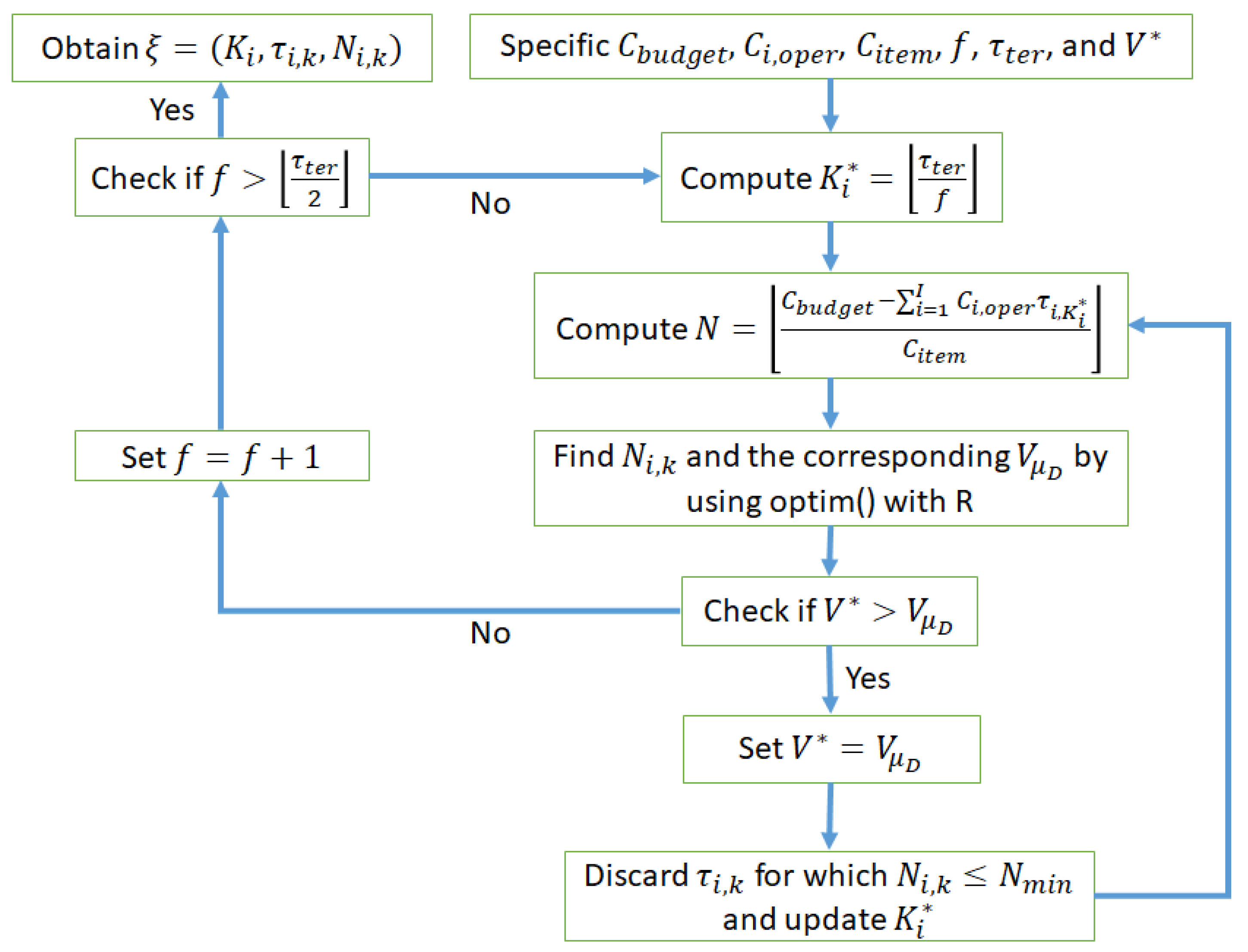
3.2. Procedure of Obtaining the Optimal CSALT Plan

Here, we assume that the cost of conducting a CSALT consists of two terms: the cost linked to the purchase of the devices and the cost associated with operation at each accelerating operating condition. In this study, it is also assumed that the operation cost increases as a result of an increase in the elevated operating condition $s_i$, as well as the duration of the CSALT, because more resources will normally be consumed to increase the elevated operating condition and conduct the CSALT for a longer duration. Given a CSALT plan $\xi =\{K_i,{\tau }_{i,k},N_{i,k},i=1,2,\cdots ,I,k=0,1\cdots ,K_i\},$ the total cost of conducting the CSALT is, therefore, given by

$$\begin{array}{c}\hfill TC\left(\xi \right)=C_{item}\sum _{i=1}^I\sum _{k=1}^{K_i}{N}_{i,k}+\sum _{i=1}^I{C}_{i,oper}{\tau }_{i,K_i},\end{array}$$

(11)

where ${\tau }_{i,K_i}$ and $C_{i,oper}$ are the duration and the operation cost, respectively, for the i-th operating condition, and $C_{item}$ is the cost of each device. Moreover, time and budget constraints are usually imposed to CSALT in practice, and therefore, the total cost $TC\left(\xi \right)$ cannot exceed a specified budget $C_{budget}$ and the duration ${\tau }_{i,K_i}$ cannot exceed a specified termination time ${\tau }_{ter}.$ In short, the optimal CSALT plan can be determined by solving the following objective function subject to time and budget constraints.

$$\begin{array}{cc}\mathrm{Minimize}\hfill & V_{{\mu }_D},\hfill \\ \mathrm{subject}\mathrm{to}\hfill & TC\left(\xi \right)\le C_{budget},\hfill \\ \hfill & {\tau }_{i,K_i}\le {\tau }_{ter},\mathrm{for}\mathrm{all}i.\hfill \end{array}$$

Figure 1 presents a framework to determine the optimal CSALT plan $\xi =\{K_i,{\tau }_{i,k},N_{i,k},$ $i=1,2,\cdots ,I,k=0,1\cdots ,K_i\}.$

Here, $\lfloor ·\rfloor$ is a truncated integer, f represents the inspection frequency, with ${\tau }_{i,k}=fk,$ and $K_i^{*}$ represents the maximum number of inspections in the i-th operating condition. It is worth noting that when the number of test groups is large, the optimization function “optim()” provides reasonable but not optimal sample sizes due to a high dimensional objective function involved in the optimization problem. Therefore, some inspection times ${\tau }_{i,k}$ are discarded if the sample sizes are very small, e.g., $N_{i,k}\le N_{min},$ so that more resources will be concentrated on the remaining test groups and the results obtained by the optimization function will be more stable due to a lower-dimensional objective function. At the same time, the duration for some operating conditions may be shortened due to the discard of inspection times, resulting in more devices being purchased for testing. It is worth noting that the median or quantile can also be used to replace the mean lifetime in the objective function. One should follow the same process in Section 3.1 to determine the corresponding asymptotic variance of the MLE.

4. Simulation Study

In this section, we perform a Monte Carlo simulation study to evaluate the performance of the procedure of obtaining the optimal CSALT plan with three stress levels $(s_1,s_2,s_3)=(35,45,55)$ under various budgets $C_{budget}\in \{\$$100,000, $200,000, $500,000$\},$ termination times ${\tau }_{ter}\in \{30,60\},$ and degrees of dependence between the components in the device $\beta \in \{0.01,0.1,0.2,0.3\},$ representing nearly independence, small dependence, moderate dependence, and high dependence, respectively.

Here, one-shot devices consisting of four components (C1, C2, C3, C4) are considered. Suppose that the cost of each one-shot device is $1100, and the costs of operation at the three stress levels are $100, $150, and $200 per unit of time, respectively. In addition, we set $(a_{10},a_{11})=(-6,0.05),(a_{20},a_{21})=(-6.5,0.06),(a_{30},a_{31})=(-7,0.07),(a_{40},a_{41})=(-8,0.08),$ and $s_0=25,$ so that the corresponding failure rates are

$$({\lambda }_1,{\lambda }_2,{\lambda }_3,{\lambda }_4)=(0.00865,0.006734,0.00525,0.00248).$$

The optimal CSALT plans for different settings are presented in

Table 1. Optimal CSALTs with various budgets $\left(C_{budget}\right),$ termination times $\left({\tau }_{ter}\right),$ and degrees of dependence $\left(\beta \right),$ along with the corresponding asymptotic variance $\left(V\right)$ and MSE for $ln\left({\mu }_D\right)$ at normal operating conditions $s_0=25.$

Setting			Optimal CSALT $\left(\mathit{\xi }\right)$			Total Cost	$ln\left({\mathit{\mu }}_{\mathit{D}}\right)$
$\mathit{\beta }$	${\mathit{C}}_{\mathit{budget}}$	${\mathit{\tau }}_{\mathit{ter}}$	${\mathit{K}}_{\mathit{i}}$	${\mathit{\tau }}_{\mathit{i},\mathit{k}}$	${\mathit{N}}_{\mathit{i},\mathit{k}}$	$\mathit{TC}\left(\mathit{\xi }\right)$	V	MSE
0.3	500K	60	(1,0,1)	(60, 0, 24)	(325, 0, 119)	499.2K	0.015	0.017
0.2	500K	60	(1,0,1)	(60, 0, 24)	(329, 0, 115)	499.2K	0.011	0.011
0.1	500K	60	(1,0,1)	(60, 0, 24)	(332, 0, 112)	499.2K	0.008	0.008
0.01	500K	60	(1,0,1)	(60, 0, 24)	(335, 0, 109)	499.2K	0.006	0.006
0.3	500K	30	(1,0,1)	(30, 0, 30)	(277, 0, 169)	499.6K	0.023	0.025
0.2	500K	30	(1,0,1)	(30, 0, 30)	(297, 0, 149)	499.6K	0.017	0.017
0.1	500K	30	(1,0,1)	(30, 0, 30)	(313, 0, 133)	499.6K	0.013	0.013
0.01	500K	30	(1,0,1)	(30, 0, 30)	(325, 0, 121)	499.6K	0.010	0.010
0.3	200K	60	(1,0,1)	(60, 0, 24)	(125, 0, 47)	200K	0.039	0.039
0.2	200K	60	(1,0,1)	(60, 0, 24)	(127, 0, 45)	200K	0.028	0.029
0.1	200K	60	(1,0,1)	(60, 0, 20)	(128, 0, 44)	199.2K	0.021	0.022
0.01	200K	60	(1,0,1)	(60, 0, 24)	(129, 0, 43)	200K	0.016	0.015
0.3	200K	30	(1,0,1)	(30, 0, 30)	(107, 0, 66)	199.3K	0.060	0.060
0.2	200K	30	(1,0,1)	(30, 0, 30)	(115, 0, 58)	199.3K	0.045	0.047
0.1	200K	30	(1,0,1)	(30, 0, 30)	(121, 0, 52)	199.3K	0.034	0.034
0.01	200K	30	(1,0,1)	(30, 0, 30)	(126, 0, 47)	199.3K	0.027	0.024
0.3	100K	60	(1,0,1)	(60, 0, 24)	(59, 0, 22)	99.9K	0.083	0.078
0.2	100K	60	(1,0,1)	(60, 0, 24)	(60, 0, 21)	99.9K	0.059	0.066
0.1	100K	60	(1,0,1)	(60, 0, 20)	(60, 0, 21)	99.1K	0.044	0.052
0.01	100K	60	(1,0,1)	(60, 0, 24)	(61, 0, 20)	99.9K	0.033	0.037
0.3	100K	30	(1,0,1)	(30, 0, 24)	(52, 0, 31)	99.1K	0.127	0.113
0.2	100K	30	(1,0,1)	(30, 0, 30)	(54, 0, 28)	99.2K	0.094	0.089
0.1	100K	30	(1,0,1)	(30, 0, 30)	(57, 0, 25)	99.2K	0.072	0.074
0.01	100K	30	(1,0,1)	(30, 0, 30)	(59, 0, 23)	99.2K	0.057	0.055

. Here, $TC$ represents the total cost of the optimal CSALT plan, $V=V_{ln\left({\mu }_D\right)}$ is the theoretical variance of the MLE for $ln\left({\mu }_D\right)$ in (7) at the normal operating condition $s_0=25,$ MSE is the mean square error (based on 1000 simulated samples) for the MLE of $ln\left({\mu }_D\right).$

First, the procedure guarantees that the total costs of the determined CSALT plans are under the corresponding budgets. Second, the theoretical and empirical variances of the MLE (V and $MSE$) are similar in all the considered cases. In general, the inspection times of the optimal CSALT plans are robust. When more devices are tested under CSALTs with a larger budget, it is not surprising that the asymptotic variance of the MLE becomes smaller. More importantly, the optimal CSALT plans require the lowest and highest stress levels. It is also observed that a long-term experiment reduces the asymptotic variance of the MLE significantly. It is recommended that more devices be placed at the lowest stress level. The dependence influences the proportions of devices being placed at the lowest and highest stress levels. When the components in devices are nearly independent, the optimal CSALT plan with a high proportion of devices placed at the lowest stress level is obtained.

In addition, we consider the income from the recycling of components under the optimal CSALT plans. It is assumed that the amounts of income generated from the recycling of components C1, C2, C3, and C4 are $100, $50, $30, and $10, respectively. For example, if failure modes $X=\{1,3\}$ are identified from a device, components C2 and C4 can then be re-sold, and the corresponding revenue from the recycling of the device is $60. However, for $X=\varnothing ,$ those devices are destroyed after successful tests, and the corresponding revenue is zero.

Table 2. Optimal CSALTs with various budgets $\left(C_{budget}\right),$ termination times $\left({\tau }_{ter}\right),$ and degrees of dependence $\left(\beta \right),$ along with the corresponding theoretical mean and standard derivation $({\mu }_R,{\sigma }_R)$ and the empirical mean and standard derivation $({\overline{x}}_R,s_R)$ of revenue from recycling the components.

Setting			Optimal CSALT $\left(\mathit{\xi }\right)$			Revenue
$\mathbf{\beta }$	${\mathit{C}}_{\mathit{budget}}$	${\mathbf{\tau }}_{\mathit{ter}}$	${\mathit{K}}_{\mathit{i}}$	${\mathit{\tau }}_{\mathit{i},\mathit{k}}$	${\mathit{N}}_{\mathit{i},\mathit{k}}$	${\mathbf{\mu }}_{\mathit{R}}$	${\overline{\mathit{x}}}_{\mathit{R}}$	${\mathit{\sigma }}_{\mathit{R}}$	${\mathit{s}}_{\mathit{R}}$
0.3	500K	60	(1,0,1)	(60, 0, 24)	(325, 0, 119)	29,995	30,114	1216	1279
0.2	500K	60	(1,0,1)	(60, 0, 24)	(329, 0, 115)	30,873	30,937	1197	1173
0.1	500K	60	(1,0,1)	(60, 0, 24)	(332, 0, 112)	31,544	31,504	1172	1112
0.01	500K	60	(1,0,1)	(60, 0, 24)	(335, 0, 109)	32,493	32,462	1146	1176
0.3	500K	30	(1,0,1)	(30, 0, 30)	(277, 0, 169)	28,817	28,854	1287	1297
0.2	500K	30	(1,0,1)	(30, 0, 30)	(297, 0, 149)	29,815	29,777	1284	1271
0.1	500K	30	(1,0,1)	(30, 0, 30)	(313, 0, 133)	30,863	30,801	1277	1265
0.01	500K	30	(1,0,1)	(30, 0, 30)	(325, 0, 121)	31,848	31,846	1266	1251
0.3	200K	60	(1,0,1)	(60, 0, 24)	(125, 0, 47)	11,618	11,641	757	728
0.2	200K	60	(1,0,1)	(60, 0, 24)	(127, 0, 45)	11,958	11,918	745	755
0.1	200K	60	(1,0,1)	(60, 0, 20)	(128, 0, 44)	12,601	12,560	734	715
0.01	200K	60	(1,0,1)	(60, 0, 24)	(129, 0, 43)	12,583	12,565	713	714
0.3	200K	30	(1,0,1)	(30, 0, 30)	(107, 0, 66)	11,173	11,176	801	834
0.2	200K	30	(1,0,1)	(30, 0, 30)	(115, 0, 58)	11,563	11,586	799	799
0.1	200K	30	(1,0,1)	(30, 0, 30)	(121, 0, 52)	11,965	11,986	795	807
0.01	200K	30	(1,0,1)	(30, 0, 30)	(126, 0, 47)	12,352	12,393	789	809
0.3	100K	60	(1,0,1)	(60, 0, 24)	(59, 0, 22)	5472	5471	519	539
0.2	100K	60	(1,0,1)	(60, 0, 24)	(60, 0, 21)	5632	5629	511	510
0.1	100K	60	(1,0,1)	(60, 0, 20)	(60, 0, 21)	5935	5936	504	514
0.01	100K	60	(1,0,1)	(60, 0, 24)	(61, 0, 20)	5927	5915	490	507
0.3	100K	30	(1,0,1)	(30, 0, 24)	(52, 0, 31)	5615	5573	560	572
0.2	100K	30	(1,0,1)	(30, 0, 30)	(54, 0, 28)	5474	5500	550	551
0.1	100K	30	(1,0,1)	(30, 0, 30)	(57, 0, 25)	5665	5657	547	534
0.01	100K	30	(1,0,1)	(30, 0, 30)	(59, 0, 23)	5840	5870	542	559

reports the theoretical mean and standard derivation $({\mu }_R,{\sigma }_R)$ and the empirical mean and standard derivation $({\overline{x}}_R,s_R)$ of revenue from recycling the components under various settings. It is realized that the theoretical and empirical results are similar. Moreover, more revenue would be generated from recycling the malfunctioned devices with independent components.

5. Eye Data from Diabetic Retinopathy Study

In this section, we consider the diabetic retinopathy study in [38]. This study examined the effectiveness of laser photocoagulation treatment in delaying the onset of blindness in patients with diabetic retinopathy. These data contain age, and the patients are classified into juveniles (aged below 20) and adults (aged 20 or above). For each patient, one eye was randomly selected for treatment and the other eye did not receive any treatment. Therefore, $M=2$ and we let $T_1$ and $T_2$ represent the time to blindness for treated and untreated eyes, respectively, and s is the age covariate that influences the time to blindness. The study showed that there is a moderate association between the treated and untreated eye for each patient. As $\beta$ is bounded between 0 and 0.5 for finite mean and variance, it is therefore reasonable to set $\beta =0.4.$ 

Table 3. Sample means of age for juvenile and adult patients and sample mean times to blindness (in months) for treated and untreated eyes of juvenile and adult patients in the eye data.

	Juvenile		Adult
Mean age	10.21		35.30
	Treated eye	Untreated eye	Treated eye	Untreated eye
Mean time to blindness	36.48	33.33	42.16	30.85

presents the sample mean times to blindness for treated and untreated eyes of juvenile and adult patients as well as the sample means of age for juvenile and adult patients. With (4), it is reasonable to set $(a_{10},a_{11})=(-3,-0.006)$ for treated eyes and $(a_{20},a_{21})=(-3,0.003)$ for untreated eyes, so that the mean times to vision loss of treated and untreated eyes for juvenile patients ($s_1=10$) are 35.55 and 32.49 months, respectively, while the mean times for adults patients ($s_2=35$) are 41.30 and 30.14 months, respectively. It is evident that the mean times to vision loss based on these settings are close to the sample means reported in Table 3.

Suppose that eye doctors check the vision of both eyes for each patient only once after receiving the treatment. There are four possible outcomes for each patient, namely, no vision loss in both eyes, vision loss in the treated eye alone, vision loss in the untreated eye alone, and vision loss in both eyes. Suppose that there is no operation cost for juvenile and adult patients ($C_{1,oper}=C_{2,oper}=\$0$), the cost of eye doctors visiting each patient is $C_{item}=\$100,$ the budget is $C_{budget}=\$$20,000, and the study allows 5 years of follow-up (${\tau }_{ter}=60$). The proposed procedure can then be used to schedule the appointments for the patients so that the asymptotic variance of the MLE of mean time to blindness for patients of age 25 ($s_0=25$) is minimized. The optimal appointment schedule is presented in

Table 4. Optimal appointment schedule for 200 patients in a 5-year study.

Patient	$\mathit{\tau }$ (months)	K
Juvenile	60	80
Adult	60	120

, which suggests that juvenile and adult patients are to be visited after receiving the treatment for 5 years and the ratio of juvenile patients to adult patients is 2:3. The asymptotic variance $V_{ln\left({\mu }_D\right)}=0.025.$

6. Concluding Remarks

In this paper, we have considered a one-shot device with dependent components having exponential lifetime distribution under gamma frailty and developed a procedure for obtaining the optimal CSALT plan with budget and time constraints. The optimal CSALT plan minimizes the asymptotic variance of the MLE for the mean lifetime under normal operating conditions. The simulation results showed that the procedure is reliable to obtain CSALT plans under specified budgets and experimental duration. Under the exponential distribution, the optimal CSALT plan requires only two stress levels. More devices are recommended to be placed at the lowest stress level. In addition, a short-term CSALT is not recommended because it results in a large variation of the MLE. The R codes can be available from the author upon request.

On the other hand, we investigate the impact of dependence between components in a device on the optimal CSALT plans. It is observed that the inspection times are robust, but more devices are placed at the highest stress level when the components are highly dependent. The dependence also influences the revenue from the recycling of the malfunctioned devices. It is found that more revenue would be generated when the components are nearly independent. Furthermore, as CSALT plans with two stress levels are the optimal design, it is natural to determine the explicit forms of the proportions of devices placed at the lowest and highest stress levels.

In this study, it is assumed that a practitioner can determine which components of the failed device have malfunctioned after a careful investigation or autopsy of the device. In some cases, some malfunctioned components may not be identified or some failure modes of interest are hindered by other failure modes, which lead to masked data or competing risk data. In this regard, it will be of practical interest to consider the analysis of one-shot devices based on masked data or competing risk data.

In addition, it will be of great interest to study optimal CSALT plans under more flexible lifetime distributions for components such as Weibull and gamma. Furthermore, the replacement of conditional independence given frailty with a conditional copula function described in [16] and the consideration of a log-linear model for the frailty variance as in [39] can be treated as extensions of this current work. We are currently working on these problems and hope to report the findings in a future paper.

References

1. Morris, M.D. A sequential experimental design for estimating a scale parameter from quantal life testing data. Technometrics 1991, 29, 173–181. [Google Scholar] [CrossRef]
2. Zhang, X.P.; Shang, J.Z.; Chen, X.; Zhang, C.H.; Wang, Y.S. Statistical inference of accelerated life testing with dependent competing failures based on copula theory. IEEE Trans. Reliab. 2014, 63, 764–780. [Google Scholar] [CrossRef]
3. Zheng, J.; Li, Y.; Wang, J.; Shiju, E.; Li, X. Accelerated thermal aging of grease-based magnetorheological fluids and their lifetime prediction. Mater. Res. Express 2018, 5, 085702. [Google Scholar] [CrossRef]
4. Balakrishnan, N.; Ling, M.H.; So, H.Y. Accelerated Life Testing of One-Shot Devices: Data Collection and Analysis; John Wiley & Sons: Hoboken, NJ, USA, 2021. [Google Scholar]
5. Balakrishnan, N.; Castilla, E.; Martín, N.; Pardo, L. Robust inference for one-shot device testing data under Weibull lifetime model. IEEE Trans. Reliab. 2019, 69, 937–953. [Google Scholar] [CrossRef]
6. Balakrishnan, N.; Castilla, E.; Martín, N.; Pardo, L. Robust inference for one-shot device testing data under exponential lifetime model with multiple stresses. Qual. Reliab. Eng. Int. 2020, 36, 1916–1930. [Google Scholar] [CrossRef]
7. Ling, M.H.; Hu, X.W. Optimal design of simple step-stress accelerated life tests for one-shot devices under Weibull distributions. Reliab. Eng. Syst. Saf. 2020, 193, 106630. [Google Scholar] [CrossRef]
8. Balakrishnan, N.; Castilla, E.; Martín, N.; Pardo, L. Divergence-based robust inference under proportional hazards model for one-shot device life-test. IEEE Trans. Reliab. 2021, 70, 1355–1367. [Google Scholar] [CrossRef]
9. Balakrishnan, N.; Castilla, E.; Ling, M.H. Optimal designs of constant-stress accelerated life-tests for one-shot devices with model misspecification analysis. Qual. Reliab. Eng. Int. 2021, in press. [CrossRef]
10. Balakrishnan, N.; Castilla, E. EM-based likelihood inference for one-shot device test data under log-normal lifetimes and the optimal design of a CSALT plan. Qual. Reliab. Eng. Int. 2021, in press. [CrossRef]
11. Zhu, X.; Liu, K.; He, M.; Balakrishnan, N. Reliability estimation for one-shot devices under cyclic accelerated life-testing. Reliab. Eng. Syst. Safety 2021, 212, 107595. [Google Scholar] [CrossRef]
12. Zhu, X.; Balakrishnan, N. One-shot device test data analysis using non-parametric and semi-parametric inferential methods and applications. Reliab. Eng. Syst. Saf. 2022, in press. [CrossRef]
13. Wang, Y.; Pham, H. Modeling the dependent competing risks with multiple degradation processes and random shock using time-varying copulas. IEEE Trans. Reliab. 2012, 61, 13–22. [Google Scholar] [CrossRef]
14. Pan, Z.; Balakrishnan, N.; Sun, Q.; Zhou, J. Bivariate degradation analysis of products based on Wiener processes and copulas. J. Stat. Comput. Simul. 2013, 83, 1316–1329. [Google Scholar] [CrossRef]
15. Peng, W.; Li, Y.F.; Yang, Y.J.; Zhu, S.P.; Huang, H.Z. Bivariate analysis of incomplete degradation observations based on inverse Gaussian processes and copulas. IEEE Trans. Reliab. 2016, 65, 624–639. [Google Scholar] [CrossRef]
16. Wang, Y.C.; Emura, T.; Fan, T.H.; Lo, S.M.; Wilke, R.A. Likelihood-based inference for a frailty-copula model based on competing risks failure time data. Qual. Reliab. Eng. Int. 2020, 36, 1622–1638. [Google Scholar] [CrossRef]
17. Liu, X. Planning of accelerated life tests with dependent failure modes based on a gamma frailty model. Technometrics 2012, 54, 398–409. [Google Scholar] [CrossRef]
18. Ling, M.H.; Ng, H.K.T.; Chan, P.S.; Balakrishnan, N. Autopsy data analysis for a series system with active redundancy under a load-sharing model. IEEE Trans. Reliab. 2016, 65, 957–968. [Google Scholar] [CrossRef]
19. Asha, G.; Raja, A.V.; Ravishanker, N. Reliability modelling incorporating load share and frailty. Appl. Stoch. Model. Bus. Ind. 2018, 34, 206–223. [Google Scholar] [CrossRef]
20. Li, Y.; Coolen, F.P.; Zhu, C.; Tan, J. Reliability assessment of the hydraulic system of wind turbines based on load-sharing using survival signature. Renew. Energy 2020, 153, 766–776. [Google Scholar] [CrossRef]
21. Meeker, W.Q.; Hahn, G.J. A comparison of accelerated test plans to estimate the survival probability at a design stress. Technometrics 1978, 20, 245–247. [Google Scholar] [CrossRef]
22. Meeker, W.Q. A comparison of accelerated life test plans for Weibull and lognormal distributions and type I censoring. Technometrics 1984, 26, 157–171. [Google Scholar] [CrossRef]
23. Escobar, L.A.; Meeker, W.Q. Planning accelerated life tests with two or more experimental factors. Technometrics 1995, 37, 411–427. [Google Scholar] [CrossRef]
24. Han, D.; Ng, H.K.T. Comparison between constant-stress and step-stress accelerated life tests under time constraint. Nav. Res. Logist. 2013, 60, 541–556. [Google Scholar] [CrossRef]
25. Wu, S.J.; Huang, S.R. Planning two or more level constant-stress accelerated life tests with competing risks. Reliab. Eng. Syst. Saf. 2017, 158, 1–8. [Google Scholar] [CrossRef]
26. Han, D. Optimal design of a simple step-stress accelerated life test under progressive type I censoring with nonuniform durations for exponential lifetimes. Qual. Reliab. Eng. Int. 2019, 35, 1297–1312. [Google Scholar] [CrossRef]
27. Fang, G.; Pan, R.; Stufken, J. Optimal setting of test conditions and allocation of test units for accelerated degradation tests with two stress variables. IEEE Trans. Reliab. 2020, 70, 1096–1111. [Google Scholar] [CrossRef]
28. Han, D. On the existence of the optimal step-stress accelerated life tests under progressive Type-I censoring. IEEE Trans. Reliab. 2019, 69, 903–915. [Google Scholar] [CrossRef]
29. Balakrishnan, N.; So, H.Y.; Ling, M.H. EM algorithm for one-shot device testing with competing risks under exponential distribution. Reliab. Eng. Syst. Saf. 2015, 137, 129–140. [Google Scholar] [CrossRef]
30. Balakrishnan, N.; So, H.Y.; Ling, M.H. EM algorithm for one-shot device testing with competing risks under Weibull distribution. IEEE Trans. Reliab. 2016, 65, 973–991. [Google Scholar] [CrossRef]
31. Balakrishnan, N.; Ling, M.H. Expectation maximization algorithm for one shot device accelerated life testing with Weibull lifetimes, and variable parameters over stress. IEEE Trans. Reliab. 2013, 62, 537–551. [Google Scholar] [CrossRef]
32. Ling, M.H.; Chan, P.S.; Ng, H.K.T.; Balakrishnan, N. Copula models for one-shot device testing data with correlated failure modes. Commun. Stat.-Theory Methods 2021, 50, 3875–3888. [Google Scholar] [CrossRef]
33. Ling, M.H.; Balakrishnan, N.; Yu, C.; So, H.Y. Inference for One-Shot Devices with Dependent k-Out-of-M Structured Components under Gamma Frailty. Mathematics 2021, 9, 3032. [Google Scholar] [CrossRef]
34. Wang, W.; Kececioglu, D.B. Fitting the Weibull log-linear model to accelerated life-test data. IEEE Trans. Reliab. 2000, 49, 217–223. [Google Scholar] [CrossRef]
35. Nayak, T.K. Multivariate Lomax distribution: Properties and usefulness in reliability theory. J. Appl. Probab. 1987, 24, 170–177. [Google Scholar] [CrossRef]
36. Johnson, N.L.; Kotz, S.; Balakrishnan, N. Continuous Univariate Distributions—Volume 1, 2nd ed.; John Wiley & Sons: New York, NY, USA, 1994. [Google Scholar]
37. Sakai, S.I.; Yoshida, H.; Hiratsuka, J.; Vandecasteele, C.; Kohlmeyer, R.; Rotter, V.S.; Yano, J. An international comparative study of end-of-life vehicle (ELV) recycling systems. J. Mater. Cycles Waste Manag. 2014, 16, 1–20. [Google Scholar] [CrossRef] [Green Version]
38. Sahu, S.K.; Dey, D.K. A comparison of frailty and other models for bivariate survival data. Lifetime Data Anal. 2000, 6, 207–228. [Google Scholar] [CrossRef]
39. Emura, T.; Sofeu, C.L.; Rondeau, V. Conditional copula models for correlated survival endpoints: Individual patient data meta-analysis of randomized controlled trials. Stat. Methods Med Res. 2021, 30, 2634–2650. [Google Scholar] [CrossRef]
Figure 1. A general framework to determine the optimal CSALT.
Mathematics 10 00840 g001