Estimating the Fractal Dimensions of Vascular Networks and Other Branching Structures: Some Words of Caution

Abstract

Branching patterns are ubiquitous in nature; consequently, over the years many researchers have tried to characterize the complexity of their structures. Due to their hierarchical nature and resemblance to fractal trees, they are often thought to have fractal properties; however, their non-homogeneity (i.e., lack of strict self-similarity) is often ignored. In this paper we review and examine the use of the box-counting and sandbox methods to estimate the fractal dimensions of branching structures. We highlight the fact that these methods rely on an assumption of self-similarity that is not present in branching structures due to their non-homogeneous nature. Looking at the local slopes of the log–log plots used by these methods reveals the problems caused by the non-homogeneity. Finally, we examine the role of the canopies (endpoints or limit points) of branching structures in the estimation of their fractal dimensions.

1. Introduction

Ever since Benoît Mandelbrot first coined the term fractal in 1975 [1], mathematicians have struggled to reach a consensus as to the formal definition of a fractal. In fact, Mandelbrot himself is purported to have proposed multiple definitions. In his book The Fractal Geometry of Nature he states

“A fractal is by definition a set for which the Hausdorff–Besicovitch dimension strictly exceeds the topological dimension.”

[2] (p. 15).

Yet, only a few years later he is said to have retracted this definition, citing it as too restrictive, and proposed the following instead:

“A fractal is a shape made of parts similar to the whole in some way.”

[3] (p. 11).

Years later, it would seem that we are no closer to having a single, precise definition for what makes something a fractal. As Kenneth Falconer so eloquently writes in the introduction to his book, Fractal Geometry,

“... the definition of a ‘fractal’ should be regarded in the same way as a biologist regards the definition of “life”. There is no hard-and-fast definition but just a list of properties characteristic of a living thing...”

[4] (p. xxvii).

Falconer goes on to list some of the typical properties of fractal sets, notably including “Often ... has some form of self-similarity, perhaps approximate or statistical.” [4] (p. xxviii). Although not a strict requirement of fractal sets, the idea of self-similarity is frequently associated with fractal theory and fractal sets. Self-similarity, or scale invariance, is frequently leveraged in order to compute fractal dimensions of such sets, either in theory via the similarity dimension, or in practice, via methods such as box-counting and the sandbox method.

In this paper we are concerned with the estimation of the fractal dimensions of a particular class of objects, namely branching structures, which are of particular interest for two reasons:

• Branching patterns are ubiquitous in nature. For example we observe branching in trees, rivers/streams, the vascular system, branching airways in the lungs, etc.
• Due to the process by which they are generated, branching structures are not strictly self-similar, yet can still have fractal properties. Fractal trees, for instance, are known to have a box-counting dimension greater than their topological dimension [2].

By looking at the local slopes which arise from the box-counting and sandbox methods, we will show that the lack of strict self-similarity (or non-homogeneity) of fractal trees and other branching structures causes the usual methods for estimating fractal dimensions to fail. Despite this, one can find many studies which use these methods to estimate the fractal dimensions of various branching structures, such as stream networks [5,6], root systems [7], and vascular networks [8]. In these studies, fractal dimension is used to characterize the complexity of branching patterns. Specifically, in the case of vascular networks, the results have been found to differentiate between healthy and diseased morphology, and have in some cases been used to draw conclusions about the fractal processes generating such networks. We propose that results such as these should be treated with skepticism because the methods used to estimate dimension rely on an assumption of self-similarity which branching structures do not satisfy.

We must point out here that we are not alone in our questioning of the indiscriminate and widespread application of fractal dimension estimation methods to images of natural objects. In 1995, as the application of fractal theory to all sorts of naturally occurring structures was becoming prevalent, the authors of [9] suggested a simpler explanation for the branching patterns observed in retinal neurons which had previously been hypothesized to be fractal. They showed, using a systematic approach, that such structures are space-filling, not fractal. Later that same year, J.D. Murray cautioned against the use of fractal measurements to draw conclusions about biological processes, noting that

“The problem with a good name for a new field is that ... inappropriate use can raise unrealistic expectations as to its relevance and applicability. This is particularly true for fractal theory which can be visually dramatic and can be practised without much background or sophistication.”

[10] (p. 369).

Adding further support to the criticisms of fractal theory, in 1996, the authors of [11] demonstrated that random distributions exhibit apparent fractal behaviour over a range of scales consistent with the typical range observed in experimental measurements of fractal objects. These early words of warning were not generally heeded, and studies on the estimation of the fractal dimensions of natural objects have continued to appear. Amidst these studies, some more recent criticisms have emerged, including [12], in which the authors discuss some of the difficulties in applying fractal methods to ecological data, concluding that evidence of a scaling relationship which spans only a few orders of magnitude is not sufficient evidence for true fractality, and [7], which cautions against computing fractal dimensions of root systems without rigorously testing for self-similarity, or statistical self-similarity, first. In this paper we move one step further, providing evidence against the application of fractal dimension estimation methods to any and all branching structures. It should be noted here that these comments extend to “multifractal” methods as well, since the determination of the famous $f\left(\alpha \right)$ curve is dependent on least-squares fitting of box-counting data and thereby suffers from the same problems we will discuss in this paper.

2. Methods for Estimating Fractal Dimensions

The two primary methods for estimating fractal dimensions from finite images seen in the literature are the box-counting method (by far the most common) and the sandbox method. These two methods are often used interchangeably to compute the “fractal dimension”; however, it is important to be aware that there are many ways to define a fractal dimension, and they are not always equivalent. The box-counting method and sandbox method compute two different dimensions: the box-counting dimension (or capacity dimension) and the correlation dimension, respectively. In some cases (when the set is a monofractal) these two definitions are equivalent; however, when working with naturally occurring objects, whether the object is monofractal, multifractal, or even if it is fractal at all, is not known at the outset.

The box-counting method: The box-counting dimension is one of the most well-known fractal dimensions due to its relatively intuitive formulation and ease of empirical estimation [4] via the aptly named box-counting method. The box-counting dimension is a measure of the rate of emergence of detail of a fractal set, and is defined [4] as

$$\begin{array}{c}\hfill D=\underset{\epsilon \to 0}{lim}{\displaystyle \frac{-log\left(N\right(\epsilon \left)\right)}{log\left(\epsilon \right)}},\end{array}$$

(1)

where $N\left(\epsilon \right)$ is the smallest number of boxes of side length $\epsilon$ which cover the set. This definition follows from the assumption that the number of boxes required to cover the set follows a power law, i.e.,

$$\begin{array}{c}\hfill N\left(\epsilon \right)=\mathcal{O}\left({\epsilon }^{-D}\right)\mathrm{as}\epsilon \to 0.\end{array}$$

(2)

In practice, finite images can, of course, only exhibit detail over a finite range of scales. As such, in the finite case, we cannot expect the scaling relationship to hold in the limit as $\epsilon \to 0$. Instead, in the finite case, we must locate the relevant range of scales over which the scaling relationship holds. Over this range of scales, the set is covered with a grid and the dimension is estimated from the slope of a log–log plot of $N\left(\epsilon \right)$ (the number of boxes which intersect the set) vs. $1/\epsilon$. The idea is that over this range of scales, we can treat the finite set as an approximation for a (statistically) self-similar set, such that the scaling relationship holds at all scales, and can effectively be extrapolated from this finite region down to the limit as $\epsilon \to 0$. We note that in the finite case we require a more strict version of the scaling relationship in Equation (2), $N\left(\epsilon \right)\propto {\epsilon }^{-D}$, in order to measure the dimension from the slope of the log–log plot. The box-counting method provides an estimate of the box-counting dimension; not of the finite set itself, but of the fractal set which it approximates [7]. In this paper we will use the notation $D_{BC}$ to refer to estimates of the box-counting dimension computed using the box-counting method.

Despite its popularity, the box-counting method is not without its flaws. For one thing, locating the correct range of scales over which the scaling relationship holds can be problematic, especially as many of the scaling relationships observed in nature span fewer than two orders of magnitude [12]. This aspect of fractal dimension estimation is mostly glossed over in the literature, and it seems that most authors simply select a region of the log–log plot of $N\left(\epsilon \right)$ vs. $1/\epsilon$ which looks reasonably linear from which to estimate dimension. Another issue is the quantization error which arises from approximating the minimum cover of the set with the number of boxes intercepted by the set using an arbitrary grid [7]. Quantization error can be reduced by translating the grid either randomly or systematically and taking the minimum $N\left(\epsilon \right)$, but there will always be some error due to the fact that we are using a fixed grid, and boxes are not allowed to shift relative to one another. Finally, box-counting suffers from what are commonly referred to as “edge effects”, referring to the boxes near the border of the set, which may intersect the set in only a minor way. At large scales, edge effects become increasingly prominent and lead to deflated estimates of dimension. Edge effects can be somewhat mitigated by enforcing a minimum density before a box is counted, or by restricting boxes to the interior of the set, as in [9]; however, this requires fairly large sets in order to be effective.

The sandbox method: The sandbox method, as described in [13], is often presented as an alternative method of estimating the fractal dimension from an image. The sandbox method is a means of estimating the correlation dimension, which is often the same, or similar to the box-counting dimension, from finite images. In the sandbox method, each occupied pixel is surrounded by a box of size $\epsilon$, and the average mass (i.e., number of pixels) inside a box of size $\epsilon$ is computed by averaging over the boxes surrounding each pixel in the set. Once again, we assume a (statistically) self-similar set, and so the average mass, $\overline{M}\left(\epsilon \right)$, is assumed to scale according to a power law, $\overline{M}\left(\epsilon \right)\propto {\epsilon }^D$, over some finite range of scales. The dimension, D, is estimated as the slope of the straight line fit to a log–log plot of $\overline{M}\left(\epsilon \right)$ vs. $\epsilon$.

The sandbox method suffers from the same issue as the box-counting method with regard to the difficulty in locating the linear region of said plot. However, since the boxes in the sandbox method are centred on individual pixels, the edge effects are less significant and we do not see the same issues as in the box-counting method with quantization error caused by the use of a fixed grid. Typically, the sandbox method is more computationally expensive than the box-counting method; however, we note that the run time of the sandbox method depends on the density of the image. Thus, for sparse images, the sandbox method can actually be quite efficient.

The generalized sandbox method:The sandbox method, as described above, is a special case of the generalized sandbox method described in [14], which computes a spectrum of generalized dimensions, $D_q$. By setting $q=2$ in the generalized sandbox method, and taking the average mass over all points in the set, we recover what is typically referred to as, simply, the sandbox method, an estimate of the correlation dimension, $D_2$. If we set $q=0$ in the generalized sandbox method, the result is another method of approximating the box-counting dimension, $D_0$.

In this paper we will present results using both the box-counting method (to compute $D_{BC}$), and the generalized sandbox method (to compute both $D_0$ and $D_2$). We implemented both methods in Matlab, using the publicly available FracLac software [15] as a baseline for our implementations. Furthermore, both methods were validated on a selection of well-known standard fractals. In our implementation of the box-counting method we employ 100 random translations of the grid to mitigate quantization error. As expected, we generally observed that the generalized sandbox method is more robust and accurate over a larger range of scales, compared to the box-counting method.

3. Fractal Analysis of Vascular Networks: A Brief Review

The blood vascular system is composed of arterial and venous trees, hierarchical branching structures which span a large range of scales and which are connected at their extremities by the capillary network, the smallest vessels. Given their complex and hierarchical structure, it is not surprising that many researchers in the medical sciences have attempted to characterize vascular networks using fractal dimension and other fractal measures. Fractal tree models have even been used to generate realistic simulations of vascular networks [16]. Furthermore, a number of pathological conditions, including cancers and degenerative diseases, lead to changes in vessel morphology and branching structure. Tumour vasculature, for example, is known to be more chaotic in appearance than healthy vasculature and the identification of tumour angiogenesis as a potential target for the treatment of certain cancers has motivated many researchers to try to understand the mechanisms by which tumour vasculature forms [8].

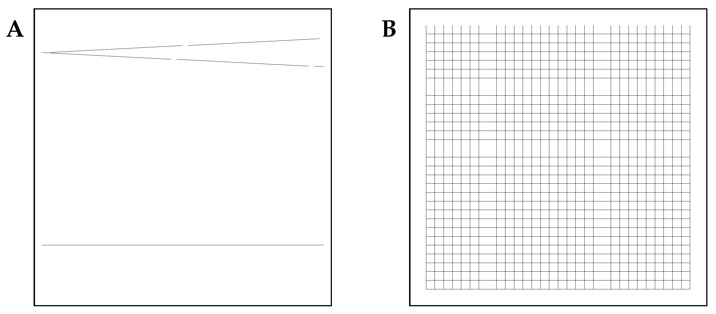
In [13,17] the authors use both the box-counting and sandbox methods to measure the fractal dimension of healthy and tumour vascular networks grown in mice bearing dorsal skinfolds. A selection of sample images from the study in [17] are shown in Figure 1, where we observe that healthy arteriovenous networks have a clear tree-like structure, healthy capillary networks have a more uniform, grid-like appearance, and tumour networks, in which arteries, veins, and capillaries cannot be distinguished, appear more disordered. The authors find good agreement between the box-counting and sandbox methods. Their measurements show that the dimension of healthy vasculature is in agreement with that of diffusion-limited aggregation ($D\approx 1.71$), while the dimension of tumour vasculature agrees with that of critical percolation clusters ($D\approx 1.896$), and capillary networks are found to have a dimension in the range 1.96–2, which is consistent with that of a two-dimensional object or a space-filling curve in two dimensions. They claim that the result for healthy vasculature is in agreement with the accepted view of the angiogenic process, whereas the results for tumour vasculature are used to form the basis of a novel hypothesis that tumour angiogenesis is a local growth process. Additional results in [13] corroborate these results, additionally showing that anti-angiogenic treatments applied to tumour vasculature lead to decreased estimates of fractal dimension. A number of further studies have been performed on both experimental images of healthy and tumour vasculature [18,19,20] as well as simulations of tumour vasculature [21,22]. These studies all tend to agree on the fractality of both healthy and tumour vasculature, and, when compared, tumour vasculature is consistently found to have a greater dimension than healthy arteriovenous networks. That being said, the specific numerical estimates of dimension across studies are somewhat less consistent. Given the inconsistencies in imaging methods, image processing methods, and in the implementations of fractal dimension estimation methods, this is not surprising. One simply has to look at the first table in [23] for an example of the variation in estimates of the fractal dimension of healthy vasculature over the years.

Fractal dimension estimation methods have also been widely applied to imaging of retinal vasculature, perhaps even more so than tumour vasculature, due to the ease of high-quality image acquisition. A number of studies have found the dimension of healthy retinal vasculature to be consistent with that of diffusion limited aggregates [25,26,27,28], in line with what was found in [17] for healthy arteriovenous networks in mice. Despite this, a fairly recent work [29] reported much lower dimensions on a fairly large database of retinal images. Some studies have also compared the retinal vasculature of cognitively healthy patients to that of patients with degenerative diseases, finding that estimates of dimension are lower for cognitively impaired patients [29,30].

We make note here of a general observation that the results in the literature tend to find that estimates of fractal dimension correlate positively with vessel density. For example, as we saw in Figure 1, tumour networks appear much more dense than healthy vasculature, and capillaries, occurring at the smallest scales, have the highest vessel density. In [31,32], a positive relationship between vessel density and estimated fractal dimension is shown directly. A correlation between density and dimension is perhaps expected, since fractal dimension is often considered a measure of how space-filling an object is. However, it turns out that in the case of branching structures, estimates of fractal dimension are directly influenced by the spacing between nearby branches and, consequently, the vessel density.

4. On the Self-Similarity (or Lack Thereof) of Fractal Trees and Other Branching Structures

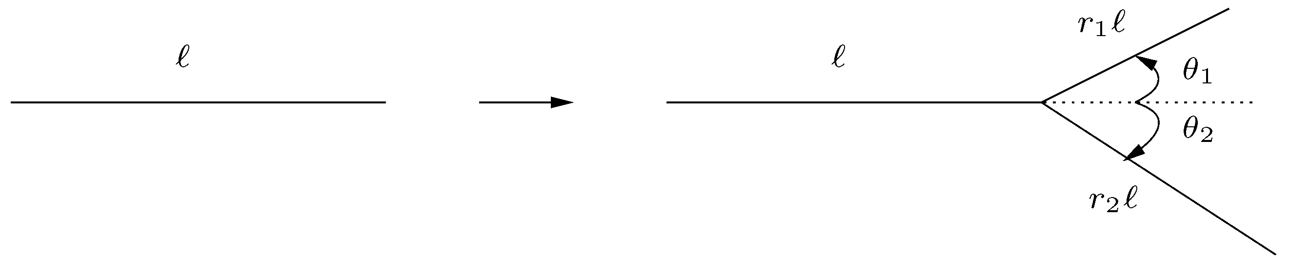
The idea of branching patterns and, more specifically, of a branching structure, is a relatively intuitive concept; however, the formal definition varies depending on the context. In this paper we consider branching structures to be a class of objects which are generated by repeated branching of a trunk (an infinitely thin line segment) into contracted and rotated copies of itself. On each iteration, a branching generator, such as the one shown in Figure 2, is applied to the branches generated in the previous step. Realistic examples of branching structures are, of course, not infinitely thin; however, in in order to focus on the structural information, images are typically skeletonized prior to estimating their fractal dimension. Some works do consider the diameters of branches in their analysis; however, similar problems in estimating the fractal dimension are found to persist regardless of whether images are skeletonized or left in their original form. We make note here of the fact that grids and grid-like structures fall into our definition of branching structures since we have not placed any restrictions on branches touching or overlapping with each other.

In the special case, where the same branching generator is applied on each iteration, as shown in Figure 3, the resulting structure possesses a kind of self-similarity. We can see from Figure 3 that if we repeat the branching process indefinitely, each sub-tree emanating off the main trunk will be a scaled and rotated copy of the tree itself. Of course, we do not expect naturally occurring branching structures, such as the vascular networks from Figure 1, to have an exact scaling relationship such as the fractal tree discussed above; however, they may possess a similar kind of statistical, or approximate, self-similarity if the branching parameters are picked from the same distribution on each iteration. Such a branching structure is commonly referred to as a fractal tree, and for certain values of the branching parameters, we can show that the fractal (box-counting) dimension is greater than the topological dimension [2,33]. At this point, it should also be stated that if the branching generator is applied only a finite number of times, the fractal (Hausdorff) dimension of the resulting tree is equal to its topological dimension, namely 1.

Although they are commonly referred to as fractals, fractal trees differ from most other examples of fractal sets. Even in the infinite case, fractal trees are not strictly self-similar (i.e., composed of a union of copies of themselves) due to the fact that the trunk remains unchanged during the generation process. At best, fractal trees can be viewed as the union of two scaled copies of themselves, plus the trunk, which can be thought of as a degenerate copy of the set, squashed infinitely thin in one direction. As a result, fractal trees are sometimes referred to as “non-homogeneous” fractals, and standard methods of computing the dimension via similarity do not apply. Instead, the tree can be considered as the union of two parts: one consisting of the trunk and the branches (which has dimension 1, equal to its topological dimension), and a second part consisting of just the branch tips, or the tree “canopy” (which is strictly self-similar, and has dimension D). When $D>1$, the canopy is dominant and the fractal dimension of the whole tree is equal to D [2]. An example is presented in Appendix A.

We note that, in practice, one can only work with finite approximations of what is assumed to be an underlying theoretical fractal set. The dimension of this theoretical set is estimated by measuring the scaling relationships over a finite number of scales. Moreover, the non-homogeneity of infinite fractal trees violates the self-similarity assumptions of the box-counting and sandbox methods, and thus impacts our ability to estimate their dimension from finite approximations. From the theoretical discussion above, one might assume that measurements of the fractal dimension of fractal trees would be underestimates of the true dimension (as a result of the tree canopy not necessarily dominating in the finite case). However, it turns out that the opposite is true due to transitions in the proportionality constant of the scaling relationship which occur at characteristic box sizes related to the density of branches in the image.

5. Local Slopes and the Proportionality Constant of the Scaling Relationship

Consider an image comprising a finite number of finite line segments which form a connected set, e.g., a branching network. Away from the edges, the mass in a box of size $\epsilon$ can always be written as $A\epsilon$, where A is some constant related to the number of line segments which pass through the box and the angle at which they pass through. If A is constant over some range of scales, then the object scales as a one-dimensional object, and this will be reflected in the results of either the box-counting or sandbox methods. Now, consider the image of a tree in Figure 3. If we cover the entire image with very small boxes, most boxes will contain a single straight line. Now imagine covering the set with slightly larger boxes—a good number of boxes will contain two (or more) line segments due to branches which are sufficiently close to each other so as to fit into a single box. In this section we investigate these transitions in the proportionality constant of the mass-scaling relationship which occur as box sizes are increased and demonstrate their effect on the results of estimating fractal dimensions directly via some simple computational examples.

5.1. Theoretical Analysis Using Local Slopes

We can use the framework of the generalized sandbox method to gain some insight into how these transitions in the mass-scaling relationship directly affect the results of estimating the box-counting and sandbox dimensions. Specifically, we consider the local slopes between two $\epsilon$ values of the log–log plot of $M\left(\epsilon \right)$ vs. $\epsilon$. The idea of looking at local slopes is not strictly ours—it has been proposed in the past as a better method for finding the linear regions of the log–log plots used in fractal dimension estimation [9,23]; however, it is has not been adopted in much of the recent literature.

In order to compute the theoretical local slopes near a transition in the mass-scaling relationship we consider an image, $\mathbf{I}$, comprising P pixels in total, and denote the mass in a box of size $\epsilon$ centred on the ith pixel by $M_i\left(\epsilon \right)$. For simplicity, assume that $\epsilon$ is small enough relative to the size of the image so that we can ignore the edge effects which result from the usual computational methods. Assume that $\mathbf{I}$ has some characteristic size ${\epsilon }^{*}$ such that when $\epsilon <{\epsilon }^{*}$ the mass-scaling relationship is constant everywhere, say $M_i\left(\epsilon \right)=A\epsilon$, and when $\epsilon >{\epsilon }^{*}$ the scaling relationship in some fraction of the boxes transitions to a new scaling relationship, $M_i\left(\epsilon \right)=B\epsilon$. Note that $A,B\ge 0$. Now, consider two box sizes, ${\epsilon }_1$ and ${\epsilon }_2$, which satisfy ${\epsilon }_1<{\epsilon }^{*}<{\epsilon }_2$. We can compute the average mass in a box of size ${\epsilon }_1$ as

$$\begin{array}{c}\hfill \begin{array}{cc}\hfill \overline{M}\left({\epsilon }_1\right)& =\frac{1}{P}\sum _{i=1}^P{M}_i\left({\epsilon }_1\right)\hfill \\ \hfill & =\frac{1}{P}·P·A{\epsilon }_1\hfill \\ \hfill & =A{\epsilon }_1.\hfill \end{array}\end{array}$$

(3)

Letting T denote the fraction of boxes in which the scaling relationship transitions, we compute the average mass in a box of size ${\epsilon }_2$ to be as follows:

$$\begin{array}{c}\hfill \begin{array}{cc}\hfill \overline{M}\left({\epsilon }_2\right)& =\frac{1}{P}\sum _{i=1}^P{M}_i\left({\epsilon }_2\right)\hfill \\ \hfill & =\frac{1}{P}\left(T·P·B{\epsilon }_2+(1-T)·P·A{\epsilon }_2\right)\hfill \\ \hfill & =T·B{\epsilon }_2+(1-T)·A{\epsilon }_2.\hfill \end{array}\end{array}$$

(4)

The dimension is estimated by computing the slope of the log–log plot of ${\overline{M}}^{(q-1)}$ vs. box size ($\epsilon$). We set $q=2$ (for the sandbox dimension) and compute the local slope between the two points ${\epsilon }_1$ and ${\epsilon }_2$, given by

$$\begin{array}{c}\hfill \begin{array}{cc}\hfill {\Delta }_2& =\frac{log\left(\overline{M}\left({\epsilon }_2\right)\right)-log\left(\overline{M}\left({\epsilon }_1\right)\right)}{log\left({\epsilon }_2\right)-log\left({\epsilon }_1\right)}\hfill \\ \hfill & =\frac{log\left(\frac{T·B{\epsilon }_2+(1-T)·A{\epsilon }_2}{A{\epsilon }_1}\right)}{log\left(\frac{{\epsilon }_2}{{\epsilon }_1}\right)}\hfill \end{array}\end{array}$$

(5)

For simplicity, we let $m=\frac{{\epsilon }_2}{{\epsilon }_1}$ so that

$$\begin{array}{c}\hfill \begin{array}{cc}\hfill {\Delta }_2& =\frac{logm}{logm}+\frac{log(T·B/A+(1-T)·A/A)}{logm}\hfill \\ \hfill & =1+\frac{log(1+T·(B-A)/A)}{logm}.\hfill \end{array}\end{array}$$

(6)

A similar argument can be made, setting $q=0$, to compute the local box-counting dimension between box sizes ${\epsilon }_1$ and ${\epsilon }_2$ as

$$\begin{array}{c}\hfill \begin{array}{cc}\hfill {\Delta }_0& =1-\frac{log(1+T·(A-B)/B)}{logm}.\hfill \end{array}\end{array}$$

(7)

From Equations (6) and (7), we can see that the local slope will be greater than 1 if B is greater than A, and less than 1 if A is greater than B. The impact of the transition on the local slope, unsurprisingly, is dependent on T, the fraction of pixels which transition, and, somewhat surprisingly, also depends on m, the ratio of the box sizes used in the algorithm. If we increase m, i.e., use box sizes which are spaced further apart, the impact of the transition on the local slope will be diminished. The results presented in this section are specific to the generalized sandbox method; however, we expect similar effects to be observed in the local slopes when applying the box-counting algorithm as well. It is not possible to write down the exact local slopes for the box-counting algorithm since the minimum number of boxes needed to cover an image depends not only on the average mass distribution, but also the spatial locations of individual pixels. That being said, the total mass of the image divided by the average mass in a box of size $\epsilon$ is a good approximation of the number of boxes required to cover the image in most cases, and so the results for $D_0$ should roughly apply to the box-counting algorithm as well.

5.2. A Few Computational Examples

We can verify the results of the previous section by constructing a simple image where a known fraction of pixels undergo a transition in the scaling relationship at a given scale, ${\epsilon }^{*}$. Such an image is shown in Figure 4. As can be seen from the magnified illustration in Figure 4B, when $\epsilon >{\epsilon }^{*}=64$ the mass-scaling relationship in the neighbourhood of the top two lines ($T=2/3$ of the total pixels) transitions from $M\left(\epsilon \right)=\epsilon$ to $M\left(\epsilon \right)=2\epsilon$. This corresponds to setting $T=2/3$, $A=1$, and $B=2$ in Equations (6) and (7). Figure 5 shows the results of applying both the generalized sandbox and box-counting algorithms to the image in Figure 4A.

A minimum box size of 3 pixels is used, and the maximum box size is set to 50 percent of the image size. Box sizes are chosen according to a power law so that ${\epsilon }_{n+1}/{\epsilon }_n\approx 1.5$. In the box-counting algorithm, 100 randomly chosen grid orientations are implemented in order to find approximately the minimum $N\left(\epsilon \right)$ for each value of $\epsilon$.

In plots A and C, the local slopes between two consecutive box sizes, ${\Delta }_2$ and ${\Delta }_0$, are compared directly with Equations (6) and (7), respectively. We observe excellent agreement between the theoretical results and the computational results from the generalized sandbox method at smaller box sizes. As the box sizes are increased, we begin to see the computational results deviate from the theory due to the edge effects which result from the computational methods. In plot E, the local slopes from the box-counting method are presented only, without any theoretical values. As expected, the behaviour of the local slopes is similar to that of the sandbox method; however, we note that the spike occurs earlier, at ${\epsilon }_2=32$ instead of 64. Unlike the sandbox method, the box-counting method does not require boxes to be centred on individual pixels, and, as such, the transition from a single line contained in a box to two lines within the same box occurs at a lower $\epsilon$ value.

Figure 5B,D,F show the log–log plots of $M\left(\epsilon \right)$, $M^{-1}\left(\epsilon \right)$, and $N\left(\epsilon \right)$, respectively, for the same image. As is usually performed, the line of best fit was computed using linear regression for each dataset, and the resulting slope (estimate of the dimension) and corresponding $r^2$ value (coefficient of determination) are presented. We note that the $r^2$ values are close to 1, which is usually interpreted as an indication of a good fit. However, as has been pointed out in [7,12,34], the independence assumption of linear regression does not hold for the box-counting or generalized sandbox methods. The quantity $M\left(\epsilon \right)$ or $N\left(\epsilon \right)$ at a given box size depends on the value at previous sizes and, consequently, when the slope is estimated using regression, the $r^2$ values are inflated and may give a false sense that the underlying data is linear. For example, all three datasets presented here look reasonably linear at first glance; however, if we take a closer look near the critical value of $\epsilon$, we can clearly see a large deviation in the slope. This local spike biases the estimate of the dimension upwards, despite the image in question clearly being one-dimensional (a finite union of one-dimensional lines). If one simply used the log–log plots to estimate the dimension of this set, as is usually performed, without considering the context added by the local slopes, the obvious conclusion would be that it is a fractal with a dimension around $D=1.1$.

Although the results in Figure 5 verify our theoretical results quite nicely, the sample image is simple and not necessarily representative of more complex branching structures. We turn our attention to two additional sample images, shown in Figure 6, for which the theoretical results would be much more difficult to write down. However, the computational results illustrate the behaviour of the local slopes of the main components present in branching structures. The pair of angled lines in Figure 6A are similar to a pair of branches emanating from a trunk in a tree-like structure, and the uniform grid in Figure 6B is similar to a more structured capillary network, not unlike Figure 1b. In Figure 7 we present the local slopes resulting from the box-counting and generalized sandbox methods applied to these two images.

In Figure 7A we see that when the two lines are placed at an angle, the local slopes gradually increase, as opposed to the single spike which we saw when they were placed at a fixed distance from each other, i.e., parallel to each other. Instead of a single large transition in the proportionality constant, we have a series of smaller transitions occurring at increasingly large scales. Eventually, we see the local slopes decrease back towards one when the box sizes are large enough that edge effects become relevant. This type of behaviour is akin to what we expect to observe in a more complex branching structure or fractal tree, but with many sets of branches of different sizes/scales, each branch causing increases in the average proportionality constant as we increase the scale.

In Figure 7B, we show the local slopes for a uniform grid with a line spacing of 32 pixels. A grid can be thought of as a special type of branching structure, in which there is no scaling (i.e., the parameter r is exactly 1) and the branches touch at a single point. Due to the lack of scaling, this set is not fractal (even if we consider an infinite number of branches); it will always be one-dimensional. At small scales, we see this reflected in the local slopes; however, as we look at scales beyond the line spacing of the grid, the local slopes rapidly increase due to transitions in the proportionality constant, eventually settling around a slope of 2. At sufficiently large scales, a grid appears to fill space in the same way as a two-dimensional object, which is consistent with the measurements on capillary networks in [9,17]. We note that the local slopes appear to approach the value 2 and then decrease as box sizes are increased further; this is due to the ever-present edge effects resulting from the use of discrete methods. Although it would not be correct to look at this plot and state that the fractal dimension of a grid (or grid-like structure) is 2, the local slopes can give us some relevant information. They tell us that beyond some characteristic scale (in this case ${\epsilon }^{*}=32$), the structure is space-filling, not fractal, which, as J.D. Murray writes, “... is a much more down to earth motivation if a branching structure is trying to maximise such things as spatial coverage without redundancy.” [10] (p. 369).

6. Estimating the Dimension of Fractal Trees

We have seen that fractal trees, and branching structures in general, are non-homogeneous, and discussed how this violates the assumptions necessary to estimate their dimensions using the standard methods. Specifically, each additional branch emanating from the trunk leads to increases in the local slopes as we look at larger and larger scales. All of this leads to the obvious conclusion that it does not make sense to apply traditional fractal dimension estimation methods to branching structures. In this section we will show via computational examples that, as expected, the box-counting and generalized sandbox algorithms do not yield accurate estimates of the fractal dimension of computer-generated fractal trees. Since it is not possible to know the theoretical dimension of real images of natural branching structures, the results in this section provide the most compelling evidence against using these methods to estimate the fractal dimensions of branching structures in general.

6.1. Fractal Trees

In Figure 8 we present plots showing the local slopes for four distinct images of finite fractal trees generated in Matlab using an iterative branching process. Each of these trees corresponds to the special case ${\theta }_1={\theta }_2=\theta$ and $r_1=r_2=r$ of the branching generator shown in Figure 2. All four trees are binary ($N=2$), and r and $\theta$ are varied. To ensure that a sufficient number of scales are present in the image, each tree contains nine generations of branches. The initial trunk length is chosen so that the lengths of the outermost branches are greater than a single pixel (in order to avoid artifacts) and, as a result, each tree approximately fills a $8192\times 8192$ image. In these plots, we once again set the minimum box size to be three pixels and the maximum at fifty percent of the image size. However, now the box sizes are incremented in a linear manner to sufficiently capture the behaviour at large scales. The local slopes are computed as the slope of a least squares fit over a range of box sizes from ${\epsilon }_1$ to ${\epsilon }_2$ (which approximately satisfy ${\epsilon }_2/{\epsilon }_1=1.5$) and plotted against the upper box size, ${\epsilon }_2$.

In the above case, for $r\ge 0.5$, the theoretical box-counting dimension of each tree is given by

$$\begin{array}{c}\hfill D={\displaystyle \frac{log\left(N\right)}{log(1/r)}}={\displaystyle \frac{log\left(2\right)}{log(1/r)}}\end{array}$$

(8)

and is indicated by a horizontal line on the corresponding plot. A derivation of this equation is presented in Appendix A. We note that when $r=0.5$ the dimension of the tree is 1; however, we still refer to it as a fractal tree as it is a limiting case. Since the trees are composed of finite line segments, at small scales, the local slopes are approximately equal to 1, as expected. Although the local slopes do pass through the true dimension of each tree briefly, we see that the slopes continue to increase well beyond this point in every case due to the transitions in the proportionality constant of the scaling relationship described in Section 5.1. At some point we see that the edge effects start to compete with the increases in slope causing somewhat of a “false plateau” at some value between 1 and 2. If we were to take this plateau as evidence of a consistent scaling relationship and estimate the fractal dimension from these plots we would significantly overestimate the true fractal dimension of these trees.

This leaves us with some obvious questions. How do we reconcile these results with the known theoretical box-counting dimension of fractal trees? Is it possible to measure this dimension from an image of the fractal tree directly, and if so, how? The scaling properties of the tree are surely encoded in an image of the tree in some way. We recall that a fractal tree can be thought of as the union of a one-dimensional object (the trunk and branches) and a D-dimensional object (the tree canopy, or “leaves”). Although the entire tree is not strictly self-similar, it is easy to show that the canopy, which is similar to a Cantor dust, is. As a result, we might expect our usual methods of estimating the dimension to be successful if applied directly to finite approximations of the tree canopy.

6.2. Fractal Tree Canopies

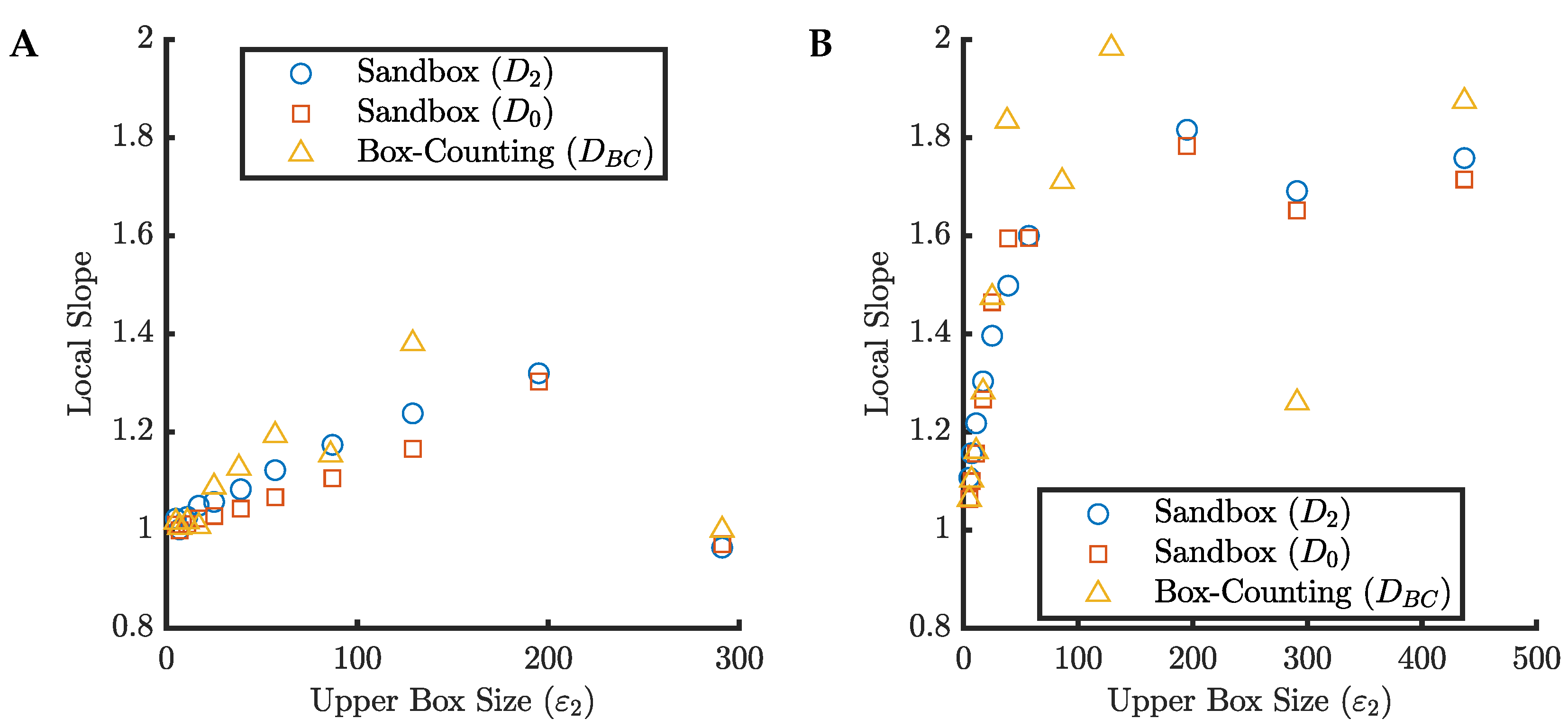
In order to construct finite approximations of the canopies corresponding to the trees shown in Figure 8, we simply extract the endpoints of the upper branches from the image of the tree itself. Each canopy image comprises exactly 512 branch tips, represented by a single pixel (or point) in the image. Figure 9 shows the local slopes plots for each fractal tree canopy. We see that at large enough scales, the local slopes hover around the true box-counting dimension of the canopy (and thus the tree itself). Once again, we used linearly spaced box sizes to generate these results and computed the local slopes over a range of box sizes satisfying ${\epsilon }_2/{\epsilon }_1\approx 1.5$. We note that the canopy images are quite sparse, so we see dips in the local slopes when the change in box sizes is small compared to the scales present in the image. In general, there is a fine balance to strike between using a lot of box sizes (and having more variability in the local slopes) and using too few box sizes (and not being able to determine if/where there is a plateau).

The examples in Figure 9 illustrate how we can estimate the fractal dimension of perfectly self-similar canopies; however, we expect the canopies of naturally occurring branching structures to be statistically self-similar at best. Figure 10 shows the same results for the box-counting and sandbox methods applied to two tree canopies generated with either r or $\theta$ chosen randomly from a uniform distribution on each iteration of the branching process. As before, we observe that at large enough scales, the local slopes hover nicely around the true box-counting dimension, even when we only have statistical self-similarity.

Based on these results, we expect that if natural branching structures are statistically self-similar, then we should be able to estimate their fractal dimensions by applying traditional methods to their canopies, if those canopies are present in the image. We propose that this might be a good alternative to current methods, while keeping the following points in mind:

• In reality, branching structures are typically three-dimensional and common practice is to produce two-dimensional images by projecting a slice of the structure onto the 2D plane. This causes overlap and disrupts the spatial organization of the canopy. To measure the dimension of a three-dimensional canopy would require 3D volumetric images, which typically are much more costly and time-consuming to generate.
• Unless a very large number of generations of branching are imaged, the tree canopy will be a very sparse set. This leads to wavy behaviour in the local slopes, as observed in Figure 9 and Figure 10, making it difficult to identify a plateau. Most real-life branching structures do not contain a particularly large number of generations, or if they do, it is at a scale too small to resolve with standard imaging techniques.
• Related to the above point, edge effects will be particularly prevalent since every point of the canopy may be considered as an edge, once again making it difficult to identify a plateau accurately. As we have seen (Figure 8), edge effects can lead to false plateaus for non-homogeneous sets.
• Finally, as was shown in [11], random distributions of points can lead to apparent fractality. As such, one should only apply fractal dimension estimation methods if there is reasonable cause to assume (statistical) self-similarity.

7. Conclusions

As we have discussed in this paper, estimating the fractal dimension of naturally occurring branching structures is a much more complex topic than previous works have suggested. Due to the process by which they are generated (which leaves the trunk unchanged), branching structures are non-homogeneous fractals at best. Thus, the usual methods of estimating fractal dimension break down due to their reliance on an assumption of self-similarity (at least over some finite range of scales). In general, these methods, such as the box-counting and sandbox methods, should not be applied to any natural object without good reason to believe that the object is, in fact, self-similar. Many claim that evidence of linearity in the log–log plot of $N\left(\epsilon \right)$ (or $M\left(\epsilon \right)$) vs. $\epsilon$ is sufficient evidence of supposed “fractal behaviour”; however, this can be misleading. For one thing, the box-counting (or sandbox) method violates the independence assumption of linear regression. This means that the usual measures of goodness of fit, such as the $r^2$ coefficient, will be inflated, and not a good indication of the linearity of the underlying data. Looking at the local slopes plots to identify a plateau over multiple scales may be better; however, as we have seen, the combination of increasing local slopes due to non-homogeneity and decreasing local slopes resulting from edge effects can lead to false plateaus at non-integer dimensions, and thus a misleading sense that the object is fractal.

Consequently, one may start to wonder if all of this is even worthwhile. How many natural objects are sufficiently self-similar over a large enough range of scales that we might have a chance to truly estimate their fractal dimensions and what do we stand to gain by doing so? It would seem that the question we really want to ask ourselves is: Why are we estimating the fractal dimension of naturally occurring objects in the first place? Once again, quoting J.D. Murray from [10], a paper which asked similar questions,

“A particular and widespread misconception about fractal theory arises because it can create objects which look remarkably like many natural structures such as trees, weeds, flowers, butterfly wing patterns and so on, and this is often taken to be a biological explanation of how these structures and patterns are formed. Although fractal-like patterns may be reasonable graphical representations of such natural shapes, they say essentially nothing about the biological processes and mechanisms which are involved in their development.”

[10] (p. 369).

Indeed, this assessment has been echoed by others, including A. Bejan, the inventor of “constructal theory”—see, for example, [35], Section 1.2, “The Hardest Questions”.

What we can say for sure is that going forward, box-counting estimates of the fractal dimension of branching networks should not be referred to as the fractal dimension of the structure or used to make claims about the processes used to generate such networks. That being said, the results from previous studies may still provide some useful information. For instance, a positive correlation has generally been observed between vessel density and estimates of the box-counting or sandbox dimension. As we have seen, analysis of the local slopes plots resulting from the box-counting and sandbox methods can provide more context regarding the spatial density of images and the presence of characteristic scales. Figure 7 and the results of [9] provide a good example of this, in which the characteristic pore size of a space-filling network is evident from the local slopes plot. In many cases, estimates of fractal dimensions were found to correlate well with some morphological property of the structure, such as distinguishing between healthy and tumour vasculature. Perhaps what this tells us is that, following the principle of Occam’s Razor, we do not need a complicated fractal theory to distinguish between such structures. Instead, perhaps a simpler measurement, such as mass density (vessel density in the case of vasculature), is sufficient to characterize complex branching networks. Of course, we can also move one step further and analyze the local scaling behaviour (i.e., local scaling exponents) of the mass density using local slopes plots, such as those shown in this paper which result from the box-counting and sandbox methods. However, in doing so, we must be careful to use the correct terminology and not use these results to infer anything about the potential fractal properties of branching structures.