Article

On Reliability Estimation of Lomax Distribution under Adaptive Type-I Progressive Hybrid Censoring Scheme

1
Department of Statistics, Faculty of Science, King Abdulaziz University, Jeddah 21589, Saudi Arabia
2
Department of Mathematics, Faculty of Science, Al-Azhar University, Cairo 11884, Egypt
3
Department of Mathematical Sciences, University of South Dakota, Vermillion, SD 57069, USA
*
Author to whom correspondence should be addressed.
Mathematics 2021, 9(22), 2903; https://doi.org/10.3390/math9222903
Submission received: 10 October 2021 / Revised: 9 November 2021 / Accepted: 13 November 2021 / Published: 15 November 2021
(This article belongs to the Special Issue Statistical Simulation and Computation II)

Abstract

:
Bayesian estimates involve the selection of hyper-parameters in the prior distribution. To deal with this issue, the empirical Bayesian and E-Bayesian estimates may be used to overcome this problem. The first one uses the maximum likelihood estimate (MLE) procedure to decide the hyper-parameters; while the second one uses the expectation of the Bayesian estimate taken over the joint prior distribution of the hyper-parameters. This study focuses on establishing the E-Bayesian estimates for the Lomax distribution shape parameter functions by utilizing the Gamma prior of the unknown shape parameter along with three distinctive joint priors of Gamma hyper-parameters based on the square error as well as two asymmetric loss functions. These two asymmetric loss functions include a general entropy and LINEX loss functions. To investigate the effect of the hyper-parameters’ selections, mathematical propositions have been derived for the E-Bayesian estimates of the three shape functions that comprise the identity, reliability and hazard rate functions. Monte Carlo simulation has been performed to compare nine E-Bayesian, three empirical Bayesian and Bayesian estimates and MLEs for any aforementioned functions. Additionally, one simulated and two real data sets from industry life test and medical study are applied for the illustrative purpose. Concluding notes are provided at the end.

1. Introduction

The distribution of lifetime random variable, X, is named as the two-parameter Lomax distribution, Lomax ( α , β ) , if its probability density function (PDF) and cumulative distribution function (CDF) are respectively defined as
f ( x ; α , β ) = α β 1 + β x ( α + 1 ) , x 0
and
F ( x ; α , β ) = 1 1 + β x α , x 0 ,
where α > 0 and β > 0 . The Lomax ( α , β ) was originally derived by Lomax [1] for the model of business failure and is also called Pareto type-II distribution. Recently, Lomax ( α , β ) has been proved to be useful in engineering, industry and medical science. For example, Hassan and Al-Ghamdi [2] utilized Lomax ( α , β ) in the reliability inference, Al-Zahrani and Al-Sobhi [3] applied Lomax ( α , β ) for the stress-strength analysis and Burkhalter and Lio [4] developed Bootstrap control charts for Lomax ( α , β ) to maintain the quality of lifetime quantiles. The reliability, R x , and hazard rate, h x , of Lomax ( α , β ) are respectively presented as
R x = 1 + β x α , x 0
and
h x = α β 1 + β x , x 0 ,
where R x illustrates the chance of an item surviving at least a specified time x and h x illustrates the likelihood of an item surviving at time x given its survival time over time x.
Since the advanced manufacturing procedure has prolonged product lifetimes, collecting life times of all items placed on life test takes longer time. Among numerous censoring schemes developed to overcome this obstacle, type-I and type-II censoring schemes have been extensively applied to the industry life test as well as medical survival analysis because of easy implementation. Given positive integers m and n with m n and τ > 0 , place n items on the failure test at the same initial time, labeled by τ 0 = 0 , and let X i : n be the lifetime of the ith failure, where i = 1 , 2 , 3 , . The type-I censoring scheme is executed till τ units of time reached; while the type-II censoring scheme is performed until the mth failure observed at X m : n . The type-I censoring scheme is called time censoring scheme and could result with less number of failure times and type-II censoring ensures a pre fixed number, m, of failure times received; however, it could be a time-consuming process. To improve the drawbacks of both schemes, Epstein [5] introduced the type-I hybrid censoring scheme that must expire at time τ = min{ X m : n , τ }; while Childs et al. [6] studied the type-II hybrid censoring scheme, which must terminate at τ = max{ X m : n , τ }. The aforementioned censoring schemes do not allow items be removed at any other time before the terminal time. In order to allow the items removed at other time points before the terminal time to save time and cost, the progressive censoring schemes have been applied to the life test. Let R i , i = 1 , 2 , , m be non-negative integers such that n = m + i = 1 m R i . The progressive type-II censoring scheme performs with n items on failure test at the same time, τ 0 = 0 , and R i items are randomly removed from remaining survival items at the ith failure, X i : n , for i = 1 , 2 , , m . Balakrishnan and Aggarwala [7] and Balakrishnan and Cramer [8] provided more information about censoring schemes and life tests. Merging the progressive type-II and hybrid censoring schemes, the type-I progressive hybrid censoring scheme that was studied by Kundu and Joarder [9] conducts the progressive type-II scheme until time τ = min{ X m : n , τ } and the type-II progressive hybrid censoring scheme, which was discussed by Childs et al. [10], implements the progressive type-II scheme up to time τ = max{ X m : n , τ }. All survival items will be removed at the respective terminated random time when the progressive hybrid censoring schemes are implemented.
Two new adaptive hybrid censoring schemes (HCSs), named as adaptive type-I progressive (AT-IP) HCS and adaptive type-II progressive (AT-IIP) HCS, have been developed recently. The AT-IIP HCS, discussed by Ng et al. [11] and Balakrishnan and Kundu [12], implements progressive type-II scheme until X m : n and has no survival items removed after the life test experiment passes τ ( < X m : n ) . The AT-IP HCS, which was shown to have a higher efficiency in estimations by Lin and Huang [13], implements progressive type-II scheme and must terminate at time τ . Let D be the number of failed items just right afore τ . If the failure time X m : n is obtained before τ , the life time experiment will continue to observe failures without withdrawing survival items until τ . Hence, at time τ , all survival items R D = n D i = 1 D R i will be removed, where R m = R m + 1 = = R D = 0 when m D ; otherwise, the AT-IP HCS uses the progressive censoring scheme R 1 , R 2 , , R D .
To deal with the selection of hyper-parameters in the Bayesian inference, Han [14,15] investigated and compared the hierarchical Bayesian and E-Bayesian methods by utilizing the quadratic loss function with three different hyper-parameters’ priors. For the E-Bayeisan estimation procedures under type-II censoring, Jaheen and Okasha [16] provided the estimates of the Burr type XII outer power parameter and reliability by means of squared error loss (SEL) and LINEX loss functions; Okasha [17] worked on the estimates of the rate parameter, parallel and series systems reliabilities and failure rate of WEI ( δ , γ ) ; and Okasha [18] investigated the estimates of Lomax distribution power parameter and reliability by means of the balanced SEL function, which was used by Ahmadi et al. [19]. Recently, Okasha and Mustafa [20] investigated E-Bayesian estimate utilizing competing risks sample from Weibull distributions under AT-IP HCS and Okasha et al. [21] extended the work by Okasha [17] to progressive type-II censoring. The common remarks of the works mentioned above indicate that the E-Bayesian estimation method outperforms over the Bayesian one. The empirical Bayesian estimation method is an alternative procedure for the hyper-parameters’ determination. Chiang et al. [22] proposed an empirical Bayesian strategy for sampling plans under Burr XII distribution. Mohammed [23] introduced an empirical E-Bayesian estimate of the Poisson distribution parameter based on random sample. Jaheen [24] studied an empirical Bayesian estimate for the exponential parameter by using Linex and quadratic loss functions based on record statistics.
Current research is an extension work by Okasha [18] for E-Bayesian estimation methods under type-II censoring. Okasha [18] did not successfully finish the mathematical proof of the comparison among the E-Bayesian estimates of Reliability under the balanced SEL function even if he obtained similar integral presentations for the difference between two E-Bayesian estimates of reliability as we did under SEL function. In our study, the SEL function as well as two asymmetric loss functions, which contain the general entropy (GE) from Calabria and Pulcini [25] and LINEX from Pandey et al. [26], will be utilized to investigate Bayesian, E-Bayesian and empirical Bayesian estimates for any function of the Lomax ( α , β ) shape parameter based on the adaptive type-I progressively hybrid censored sample.
The rest of this paper is organized as follows. In Section 2, the likelihood model and maximum likelihood estimates based on a given adaptive type-I progressively hybrid censored sample will be presented. Section 3 will discuss and formulate the Bayesian estimates of the Lomax shape functions and Section 4 will provide detail derivation of the E-Bayesian estimates. Section 5 addresses empirical Bayesian estimation procedure. The mathematical properties of all the E-Bayesian estimates are developed in Section 6. In Section 7, an extensive Monte Carlo simulation will be performed to investigate the performance of all estimates considered. Following that, one simulated data set and two practical data sets will be utilized for the illustrative purpose. Some notes will be addressed at the end.

2. Maximum Likelihood Estimation

Let Φ = x j : n , j = 1 , 2 , 3 , , D be the adaptive type-I progressively hybrid censored sample that was collected by using the progressive type-II censoring scheme, R j , j = 1 , 2 , 3 , , D , and τ . The likelihood model and maximum likelihood estimate (MLE) of any function, η ( α ) , of α , are addressed as follows.

2.1. Likelihood Model

Let Θ = ( α , β ) be the Lomax ( α , β ) parameter vector. If D = 0 , then the likelihood function is L ( Θ ; Φ ) = ( 1 F ( τ ; Θ ) ) n ; otherwise, the likelihood function of Φ is presented by
L ( Θ ; Φ ) = C D j = 1 D f ( x j : n ; α , β ) [ 1 F ( x j : n ; α , β ) ] R j [ 1 F ( τ ; α , β ) ] R D ,
where C D = i = 1 D γ i , γ i = k = i m ( R k + 1 ) = n k = 1 i 1 ( R k + 1 ) , k = 1 0 ( R k + 1 ) 0 and R D = n D j = 1 D R j . When the sample is collected from Lomax ( α , β ) , the likelihood function of (5), based on (1) and (2), can be represented as L ( α , β ; Φ ) = 1 + β τ α n for D = 0 ; otherwise, the likelihood function of (5) can be represented as,
L ( α , β ; Φ ) = C D α D b 1 ( Φ ; β ) e α T 1 ,
where
b 1 ( Φ ; β ) = β D i = 1 D 1 + β x i : n 1
and
T 1 = i = 1 D ( R i + 1 ) ln 1 + β x i : n + R D ln 1 + β τ .
It can be seen that the explicit forms of the MLE and Bayesian estimates for the rate parameter, β , are not available. Moreover, it is very common to assume one parameter as a known constant in the investigation of Bayesian and E-Bayesian estimates. For more information, readers may refer to Han [14,15], Jaheen and Okasha [16], Okasha [17] and Okasha et al. [21]. In this work, the rate parameter β is assumed to be a known constant.

2.2. Maximum Likelihood Estimator

In order to derive the MLE of any function η ( α ) based on Φ from Lomax ( α , β ) , the log-likelihood function is obtained as l L α = α n ln 1 + β τ for D = 0 ; otherwise, the log-likelihood function is presented as follows,
l L α = ln ( C D ) + D ln α + D ln β i = 1 D ln 1 + β x i : n α T 1 .
Therefore, if D = 0 then the MLE cannot be obtained; otherwise, the MLE of α can be easily derived as
α ^ ML = D T 1 ,
where T 1 is given by (7). The MLE of η ( α ) can be obtained by plug-in method and labeled by η ^ ML = η ( α ^ ML ) . Replacing α in (3) and (4) by (8), the MLEs of R x and h x at x can be derived as R ^ ML x = 1 + β x α ^ ML and h ^ ML x = α ^ ML β 1 + β x , respectively.

3. Bayesian Estimation of the Reliability Performances (BE)

In this section, the SEL function as well as GE and LINEX loss functions will be used to develop the Bayesian estimates of η ( α ) based on Φ from Lomax ( α , β ) . To develop Bayesian estimation methods, the framework that includes posterior distribution and loss function is needed.

3.1. Posterior Distribution

Since α > 0 , the flexible Gamma PDF of α , defined as
g ( α ) = k c Γ ( c ) α c 1 e k α , α 0 ,
where c > 0 and k > 0 are called hyper-parameters, will be used as a conjugate prior PDF to develop the Bayesian estimates of η ( α ) . Combining the likelihood of (6) and the prior of (9), the posterior PDF for α , given Φ , can be obtained as
π ( α | Φ ) = g ( α ) L ( α ; Φ ) 0 g ( α ) L ( α ; Φ ) d α = B 1 ( c , k ) α D + c 1 e k + T 1 α ,
where
B 1 ( c , k ) = ( k + T 1 ) D + c Γ ( D + c ) ,
and T 1 is (7). Let η : = η ( α ) . By using transformation method on PDF of (10), the posterior PDF of η can be obtained. Using R ( x ) and h ( x ) as examples, the respective transformation procedures are addressed next.
Let R x : = R ( x ) . By utilizing transformation method with α = ln R x ln ( 1 + β t ) and the PDF of (10), the posterior PDF of R x can be derived as
ψ ( R x | Φ ) = B 1 ( c , k ) ln ( 1 + β x ) D + c R x k + T 1 ln ( 1 + β x ) 1 ln R x D + c 1 , 0 < R x 1 .
Let h x : = h ( x ) . Again, by Transformation method with α = 1 + β x β h x and the PDF of (10), the posterior PDF of h x can be presented as
φ ( h x | Φ ) = B 1 ( c , k ) 1 + β x β D + c h x D + c 1 e ( k + T 1 ) ( 1 + β x ) β h x , h x 0 .

3.2. Loss Functions

When SEL function is used, the Bayesian estimate of η ( α ) is the posterior mean of η ( α ) . Therefore, we only address asymmetric loss functions in this section. Pandey et al. [26] indicated that using asymmetric loss functions would be suitable in some applications and proposed LINEX loss function. In this section, GE and LINEX loss functions will be discussed briefly. Let θ : η ( α ) and θ ^ be a Bayesian estimate of θ . For b 0 , the LINEX loss function is given as
L 1 ( θ ^ , θ ) = e b θ ^ θ b θ ^ θ 1 .
From (13), it can be noted when b > 0 , underestimation is less serious than overestimation; while b < 0 , the conclusion is opposite. When b approaches zero, the LINEX loss will be approximated to the SEL. The posterior expectation of (13) can be derived as
E θ L 1 ( θ ^ , θ ) | Φ = e b θ ^ E θ e b θ | Φ b θ ^ + b E θ θ | Φ 1 , b 0 ,
where E θ e b θ | Φ is the posterior expectation taken over the posterior of θ . The Bayesian estimate of θ , labeled by θ ^ BL , is the minimizer of (14) and can be proved to be
θ ^ BL = 1 b ln E θ e b θ | Φ ,
provided that E θ e b θ | Φ is finite.
In many practical situations, the loss in terms of the ratio θ ^ / θ could be more realistic. Under this situation, the GE loss of Calabria and Pulcini (1996) is a suitable one and defined as
L 2 ( θ ^ , θ ) θ ^ / θ p p log θ ^ / θ 1 .
When p = 1 , the GE loss function is reduced to the Entropy loss function, which has been utilized by numerous authors. More information, reader can refer to Soliman [27]. When p > 0 , overestimate is more serious than underestimate. Similarly, the Bayesian estimate, θ ^ BG , of θ for the GE loss function is defined as the minimizer of the posterior expectation, E θ L 2 ( θ ^ , θ ) | Φ , and can be proved as
θ ^ BG = E θ θ p | Φ 1 / p ,
provided that the posterior expectation, E θ θ p | Φ , is finite. In order to implement the Bayesian estimation method on any function θ : η ( α ) , more detail structure of θ is needed. Three special cases of θ will be used for the following:

3.3. Bayesian Estimate under SEL Function

The Bayesian estimates of α , R ( x ) and h ( x ) under SEL function will be presented here. The Bayesian estimate of α is the expectation of posterior distribution of (10) and given as
α ^ BS = E α | Φ = D + c k + T 1 .
The Bayesian estimate of R ( x ) is the expectation of posterior distribution of (11) and given as
R ^ BS ( x ) = 1 + ln 1 + β x k + T 1 D c ,
and the Bayesian estimate of h ( x ) is the mean of posterior distribution of (12) and given as
h ^ BS ( x ) = β 1 + β x D + c k + T 1 .

3.4. Bayesian Estimate under LINEX Loss Function

The Bayesian estimates of α , R ( x ) and h ( x ) under LINEX loss function will be provided here. Using (10) and (15), the Bayesian estimate of α is obtained as
α ^ BL = 1 b ln E α ( e b α | Φ ) = 1 b ln ( k + T 1 ) D + c Γ ( D + c ) 0 e b α α D + c 1 e k + T 1 α d α = D + c b ln 1 + b k + T 1 .
Using (11) and (15), the Bayesian estimate of R ( x ) is given by
R ^ BL ( x ) = 1 b ln E R x e b R x | Φ = 1 b ln B 1 ( c , k ) ln ( 1 + β x ) D + c 0 1 e b R x R x k + T 1 ln ( 1 + β x ) 1 ( ln R x ) ( D + c 1 ) d R x = 1 b ln j = 0 ( b ) j Γ ( j + 1 ) 1 + j ln ( 1 + β x ) k + T 1 ( D + c ) .
Using (12) and (15), the Bayesian estimate of h ( x ) is
h ^ BL ( x ) = 1 b ln E h x e b h x | Φ = 1 b ln 0 e b h x φ ( h x | Φ ) d h x = D + c b ln 1 + b β ( k + T 1 ) ( 1 + β x ) .

3.5. Bayesian Estimate under GE Loss Function

The Bayesian estimates of α , R ( x ) and h ( x ) under GE loss function will be presented as follows. Using (10) and (17), the Bayesian estimate of α is given as
α ^ BG = 1 k + T 1 Γ D + c Γ D + c p 1 / p .
Using (11) and (17), the Bayesian estimate of R ( x ) is
R ^ BG ( x ) = 1 p ln 1 + β x k + T 1 D + c p .
Using (12) and (17), the Bayesian estimate of h ( x ) is
h ^ BG ( x ) = β k + T 1 1 + β x Γ D + c Γ D + c p 1 / p .

4. E-Bayesian Estimation of the Reliability Performances

It can be noted that all Bayesian estimates mentioned above are functions of c and k, given Φ from Lomax ( α , β ) . Han [14] suggested the selection of hyper-parameters c and k to ensure that the prior PDF g ( α | c , k ) of (9) decreases when α > 0 increases. The derivative of g ( α | c , k ) with α is
d g ( α ) d α = k c Γ ( c ) α c 2 e k α [ ( c 1 ) k α ] .
Then the prior PDF, g ( α | c , k ) , is a decreasing function of α > 0 , if 0 < c < 1 and k > 0 . It is very common to assume the independence of c and k random variables. Let c and k have PDFs, π 1 ( c ) and π 2 ( k ) , respectively. Therefore, the join bivariate PDF of c and k can be represented by
π ( c , k ) = π 1 ( c ) π 2 ( k ) ,
and the expectation of the Bayesian estimate (E-Bayesian estimate) for η ( α ) can be expressed as
η ^ EB ϱ η ^ BE ( c , k ) π ( c , k ) d c d k ,
where ϱ is the domain of c and k such that the prior PDF of (9) is decreasing in α and η ^ BE ( c , k ) is any Bayesian estimate of η ( α ) . For more details about E-Bayesian, readers may refer to References [15,16,17,18,20,21,28,29].
In order to investigate the E-Bayesian estimate of η ( α ) , the structure of η ( α ) and the joint prior distribution of hyper-parameters must be specified. For illustration, we use the following three joint PDFs,
π 1 ( c , k ) = 1 ω B ( r , s ) c r 1 ( 1 c ) s 1 , 0 c 1 , 0 k ω , π 2 ( c , k ) = 2 ω 2 B ( r , s ) ( ω k ) c r 1 ( 1 c ) s 1 , 0 c 1 , 0 k ω , π 3 ( c , k ) = 2 k ω 2 B ( r , s ) c r 1 ( 1 c ) s 1 , 0 c 1 , 0 k ω ,
where r > 0 , s > 0 and B ( r , s ) is Beta function, as three different joint priors of hyper-parameters and aforementioned three η ( α ) functions, α , R ( x ) and h ( x ) .

4.1. E-Bayesian Estimates with SEL Function

Replacing η ^ B E in (27) by (18), (19), or (20) and using three priors of (28), the E-Bayesian estimates of α , R ( x ) and h ( x ) under SEL will be addressed as follows.
Using (18), (27) and three priors of (28), the E-Bayesian estimates of α based on SEL can be obtained as
α ^ E B S 1 = ϱ α ^ BS ( c , k ) π 1 ( c , k ) d k d c = 1 ω B ( r , s ) 0 1 0 ω D + c k + T 1 c r 1 ( 1 c ) s 1 d k d c = 1 ω D + r r + s ln 1 + ω T 1 ,
α ^ E B S 2 = 2 ω 2 D + r r + s ( T 1 + ω ) ln 1 + ω T 1 ω
and
α ^ E B S 3 = 2 ω 2 D + r r + s T 1 ln T 1 T 1 + ω + ω ,
respectively.
Using (19), (27) and three priors of (28), the E-Bayesian estimates of R ( x ) based on SEL can be respectively derived as
R ^ E B S 1 ( x ) = ϱ R ^ BS ( x ) π 1 ( c , k ) d k d c = 1 ω B ( r , s ) 0 1 0 ω 1 + ln 1 + β x k + T 1 D c c r 1 ( 1 c ) s 1 d k d c . = 1 ω B ( r , s ) 0 ω 1 + ln 1 + β x k + T 1 D 0 1 e c ln 1 + ln 1 + β x k + T 1 c r 1 ( 1 c ) s 1 d c d k = 1 ω 0 ω 1 + ln 1 + β x k + T 1 D F 1 : 1 r ; r + s ; ln k + T 1 k + T 1 + ln 1 + β x d k ,
R ^ E B S 2 ( x ) = 2 ω 2 0 ω ( ω k ) 1 + ln 1 + β x k + T 1 D × F 1 : 1 r ; r + s ; ln k + T 1 k + T 1 + ln 1 + β x d k
and
R ^ E B S 3 ( x ) = 2 ω 2 0 ω k 1 + ln 1 + β x k + T 1 D F 1 : 1 r ; r + s ; ln k + T 1 k + T 1 + ln 1 + β x d k ,
where F 1 : 1 . , . ; . is the generalized hypergeometric function. More information, reader may refer to Gradshteyn and Ryzhik [30]. The above estimates cannot be computed analytically. Therefore, it may be obtained numerically using the mathematical packages Matlab.
Using (20), (27) and three priors of (28), the E-Bayesian estimates of h ( x ) based on SEL can be expressed as
h ^ E B S 1 ( x ) = ϱ h ^ BS ( x ) π 1 ( c , k ) d k d c = 1 ω B ( r , s ) 0 1 0 ω β 1 + β x D + c k + T 1 c r 1 ( 1 c ) s 1 d k d c = β 1 + β x ω B ( r , s ) 0 1 0 ω D + c k + T 1 c r 1 ( 1 c ) s 1 d k d c = 1 ω β 1 + β x D + r r + s ln 1 + ω T 1 ,
h ^ E B S 2 ( x ) = 2 ω 2 D + r r + s β 1 + β x ( T 1 + ω ) ln 1 + ω T 1 ω
and
h ^ E B S 3 ( x ) = 2 ω 2 D + r r + s β 1 + β x T 1 ln T 1 T 1 + ω + ω ,
respectively.

4.2. E-Bayesian Estimates with LINEX Loss Function

Replacing η ^ B E in (27) by (21), (22), or (23) and using three priors of (28), the E-Bayesian estimates of α , R ( x ) and h ( x ) using LINEX loss are addressed below.
Using (21), (27) and three priors of (28), the E-Bayesian estimates of α based on LINEX loss function can be obtained as
α ^ E B L 1 = ϱ α ^ BL ( c , k ) π 1 ( c , k ) d k d c = 1 ω B ( r , s ) 0 1 0 ω D + c b ln 1 + b k + T 1 c r 1 ( 1 c ) s 1 d k d c = 1 ω b D + r r + s ω ln 1 + b ω + T 1 + ( T 1 + b ) ln 1 + ω T 1 + b T 1 ln 1 + ω T 1 ,
α ^ E B L 2 = D + r r + s 1 b ln 1 + b T 1 ( T 1 + ω ) 2 ω 2 b ln 1 + ω T 1 + ( T 1 + b + ω ) 2 ω 2 b × ln 1 + ω T 1 + b 1 ω
and
α ^ E B L 3 = D + r r + s 1 b ln 1 + b ω + T 1 + T 1 2 ω 2 b ln 1 + ω T 1 ( T 1 + b ) 2 ω 2 b × ln 1 + ω T 1 + b + 1 ω ,
respectively.
Using (22), (27) and three priors of (28), the E-Bayesian estimates of the reliability based on LINE loss function can be derived as
R ^ E B L i ( x ) = ϱ R ^ BL ( x ) π i ( c , k ) d k d c ,
for i = 1 , 2 , 3 , respectively. The integral results in (41) are very complicated and the explicit forms are difficult to obtain. Computations with a software can be applied to evaluate the E-Bayesian estimates of reliability.
Using (23), (27) and three priors of (28), the E-Bayesian estimates of the hazard rate based on LINEX loss function can be respectively expressed as
h ^ E B L 1 ( x ) = ϱ h ^ BL ( c , k ) π 1 ( c , k ) d k d c = 1 ω B ( r , s ) 0 1 0 ω D + c b ln 1 + b β ( k + T 1 ) ( 1 + β x ) c r 1 ( 1 c ) s 1 d k d c = 1 ω b D + r r + s z ( x , b , β ) ln 1 + ω T 1 + z ( x , b , β ) + ( T 1 + ω ) × ln 1 + z ( x , b , β ) T 1 + ω T 1 ln 1 + z ( x , b , β ) T 1 ,
h ^ E B L 2 ( x ) = 1 b D + r r + s 1 + T 1 + z ( x , b , β ) ω 2 ln 1 + ω T 1 + z ( x , b , β ) 1 + T 1 ω 2 1 + ln ω T 1 + ln 1 + z ( x , b , β ) T 1 z ( x , b , β ) ω
and
h ^ E B L 3 ( x ) = 1 b D + r r + s T 1 ω 2 ln 1 + ω T 1 T 1 + z ( x , b , β ) ω 2 × ln 1 + ω T 1 + z ( x , b , β ) + ln 1 + z ( x , b , β ) T 1 + ω + z ( x , b , β ) ω ,
where z ( x , b , β ) = b β 1 + β x .

4.3. E-Bayesian Estimates with GE Loss Function

Replacing η ^ B E in (27) by (24), (25), or (26) and using three priors of (28), the E-Bayesian estimates of α , R ( x ) and h ( x ) using GE loss will be described as follows.
Using (24), (27) and three priori of (28), the E-Bayesian estimates of α based on GE loss can be respectively obtained as
α ^ E B G E 1 = ϱ α ^ GE ( c , k ) π 1 ( c , k ) d k d c = 1 ω B ( r , s ) 0 1 0 ω 1 k + T 1 Γ D + c Γ D + c p 1 / p c r 1 ( 1 c ) s 1 d k d c = I 1 ( D , p ) ω B ( r , s ) ln 1 + ω T ,
α ^ E B G E 2 = 2 I 1 ( D , p ) ω 2 B ( r , s ) ( T + ω ) ln 1 + ω T ω
and
α ^ E B G E 3 = 2 I 1 ( D , p ) ω 2 B ( r , s ) ω T log 1 + ω T ,
where
I 1 ( D , p ) = 0 1 Γ D + c Γ D + c p 1 / p c r 1 ( 1 c ) s 1 d c .
Using (25), (27) and three priors of (28), the E-Bayesian estimates of R ( x ) based on GE loss can be respectively expressed as
R ^ E B G E 1 ( x ) = ϱ R ^ GE ( x ) π i ( c , k ) d k d c = 1 ω B ( r , s ) 0 1 0 ω 1 p ln 1 + β x k + T 1 D + c p c r 1 ( 1 c ) s 1 d k d c = Γ ( r + s ) ω 0 ω ψ ( k , x ) d k ,
R ^ E B G E 2 ( x ) = 2 Γ ( r + s ) ω 2 0 ω ( ω k ) ψ ( k , x ) d k
and
R ^ E B G E 3 ( x ) = 2 Γ ( r + s ) ω 2 0 ω k ψ ( k , x ) d k ,
where
ψ ( k , x ) = 1 p ln 1 + β x k + T 1 D p F 1 : 1 r , r + s ; 1 p ln 1 p ln 1 + β x k + T 1 .
The respective explicit forms of (49)–(51) cannot be obtained. It may be obtained numerically using the mathematical packages Matlab.
Using (26), (27) and three priors of (28), the E-Bayesian estimates of h ( x ) based on GE loss can be respectively expressed as
h ^ E B G E 1 ( x ) = ϱ α ^ B L ( c , k ) π 1 ( c , k ) d k d c = 1 ω B ( r , s ) 0 1 0 ω β k + T 1 1 + β x Γ D + c Γ D + c p 1 / p × c r 1 ( 1 c ) s 1 d k d c = I 1 ( D , p ) ω B ( r , s ) β 1 + β x ln ( 1 + ω T 1 ,
h ^ E B G E 2 ( x ) = 2 I 1 ( D , p ) ω 2 B ( r , s ) β 1 + β x ( ω + T 1 ) ln ( 1 + ω T 1 ω
and
h ^ E B G E 3 ( x ) = 2 I 1 ( D , p ) ω 2 B ( r , s ) β 1 + β x ω T 1 ln 1 + ω T 1 ,
where I 1 ( D , p ) had been defined in (48). The explicit forms of (52)–(54) cannot be derived. It may be obtained numerically using the mathematical packages Matlab.

5. Empirical Bayesian Estimates of the Reliability Performances

We will develop an alternative technique that is called empirical Bayesian estimation method to tackle the unknown hyper-parameters in this section.

5.1. Estimation Method for Hyper-Parameters

The MLE has been known usually more accurate than any other estimate (for example, moment estimate). Based on this fact, Yan and Gendai [31] proposed the MLEs of hyper-parameters to analyze the Bayesian reliability indexes. The current study, the Gamma prior of (9) has the hyper-parameters c and k. The maximum likelihood method will be applied to estimate the hyper-parameters, c and k, based on Φ .
Using (1) and the prior PDF (9) of α , the margin PDF of X can be derived as follows,
f ( x ) = 0 f ( x ; α , β ) g ( α ) d α = c k c β ( 1 + β x ) k + ln ( 1 + β x ) c + 1
and
1 F ( x ) = x f ( t ) d t = k k + ln ( 1 + β x ) c .
Replacing f ( x ; α , β ) by f ( x ) and F ( x ; α , β ) by F ( x ) , the likelihood function of (5) can be represented as
L 2 ( c , k ; Φ ) = C D c D b 2 ( Φ ; β ) e c T 2 ,
where
b 2 ( Φ ; β ) = β D i = 1 D ( 1 + β X i : n ) ( k + ln ( 1 + β X i : n ) )
and
T 2 ( k ) = i = 1 D ( R i + 1 ) ln k + ln ( 1 + β X i : n ) + R D ln k + ln 1 + β τ n ln k .
The log-likelihood function using (55) can be addressed as
lL 2 ( c , k ; Φ ) = ln ( C D ) + D ln ( c ) + D ln ( β ) i = 1 D ln 1 + β X i : n i = 1 D ln k + ln ( 1 + β X i : n c T 2 ( k ) .
Setting the partial derivatives of (56) with respect to c and k equal to 0, respectively, the normal equations are derived to be
c = D T 2 ( k )
and
c n k = i = 1 D c ( R i + 1 ) + 1 k + ln ( 1 + β X i : n ) + R D k + ln ( 1 + β τ ) ,
where T 2 ( k ) is given by (55). The solutions, c ^ and k ^ , of c and k from (57) and (58), simultaneously, are the MLEs of c and k, respectively. Therefore, the empirical Bayesian estimate of η ( α ) will be obtained via replacing c and k in η ^ BE ( c , k ) with c ^ and k ^ . In this section, the empirical Bayesian estimates for all Bayesian estimates mentioned before will be presented as follows,

5.2. Empirical Bayesian Estimates under SEL

The empirical Bayesian estimates of α ^ B S , R ^ B S ( x ) and h ^ B S ( x ) using SEL can be presented as
α ^ E M B S = D + c ^ k ^ + T 2 ( k ^ ) ,
R ^ E M B S ( x ) = 1 + ln 1 + β x k ^ + T 2 ( k ^ ) D c ^
and
h ^ E M B S ( x ) = β 1 + β x D + c ^ k ^ + T 2 ( k ^ ) ,
respectively.

5.3. Empirical Bayesian Estimates under LINEX Loss

The empirical Bayesian estimates of α ^ B L , R ^ B L ( x ) and h ^ B L ( x ) under LINEX loss can be addressed as
α ^ E M B L = D + c ^ b ln 1 + b k ^ + T 2 ( k ^ ) ,
R ^ E M B L ( x ) = 1 b ln j = 0 ( b ) j Γ ( j + 1 ) 1 + j ln ( 1 + β x ) k ^ + T 2 ( k ^ ) ( D + c ^ )
and
h ^ E M B L ( x ) = D + c ^ b ln 1 + b β ( k ^ + T 2 ( k ^ ) ) ( 1 + β x ) ,
respectively.

5.4. Empirical Bayesian Estimates under GE Loss

The empirical Bayesian estimates of α ^ B G , R ^ B G ( x ) and h ^ B G ( x ) under GE Loss are presented as
α ^ E M B G = 1 k ^ + T 2 ( k ^ ) Γ D + c ^ Γ D + c ^ p 1 / p ,
R ^ E M B G ( x ) = 1 p ln 1 + β x k ^ + T 2 ( k ^ ) D + c ^ p
and
h ^ E M B G ( x ) = β k ^ + T 2 ( k ^ ) 1 + β x Γ D + c ^ Γ D + c ^ p 1 / p ,
respectively.

6. Properties of E-Bayesian Estimates

In order to derive the properties for E-Bayesian estimates of η ( α ) , more conditions or structures on η ( α ) are needed. However, the general conditions are not available. Therefore, the aforementioned functions will be focused. Some relationships among all E-Bayesian estimates mentioned above will be established in this section.

6.1. Properties of E-Bayesian Estimates under SEL

Some relationships among α ^ E B S j , R ^ E B S j ( x ) and h ^ E B S j ( x ) ( j = 1 , 2 , 3 ) are given by Propositions 1–3.
Relationships among α ^ E B S j ( j = 1 , 2 , 3 )
Proposition 1.
Let r > 0 , s > 0 , 0 < ω < T 1 and α ^ E B S j ( j = 1 , 2 , 3 ) be presented by (29), (30) and (31). Then
(i) 
α ^ E B S 3 < α ^ E B S 1 < α ^ E B S 2 .
(ii) 
lim T 1 α ^ E B S 1 = lim T 1 α ^ E B S 2 = lim T 1 α ^ E B S 3 .
Proof. 
(i) From (29)–(31),
α ^ E B S 2 α ^ E B S 1 = α ^ E B S 1 α ^ E B S 3 = 1 ω D + r r + s ω + 2 T 1 ω ln T 1 + ω T 1 2 .
When 1 < t < 1 , ln ( 1 + t ) = t t 2 2 + t 3 3 t 4 4 + = i = 1 ( 1 ) i t i i .
Let t = ω T 1 . Since 0 < ω < T 1 and 0 < ω T 1 < 1 ,
ω + 2 T 1 ω ln 1 + ω T 1 2 = ω + 2 T 1 ω ω T 1 1 2 ω T 1 2 + 1 3 ω T 1 3 1 4 ω T 1 4 + 1 5 ω T 1 5 2 = ω T 1 1 2 ω T 1 2 + 1 3 ω T 1 3 1 4 ω T 1 4 + 1 5 ω T 1 5 2 + ( 2 ω T 1 + 2 3 ω T 1 2 2 4 ω T 1 3 + 2 5 ω T 1 4 ) = ω 2 6 T 1 2 ω 3 6 T 1 3 + 3 ω 4 20 T 1 4 2 ω 5 15 T 1 5 + = ω 2 6 T 1 2 1 ω T 1 + ω 4 300 T 1 4 45 40 ω T 1 + > 0 .
According to (68) and (69), we have
α ^ E B S 2 α ^ E B S 1 = α ^ E B S 1 α ^ E B S 3 > 0 ,
that is
α ^ E B S 3 < α ^ E B S 1 < α ^ E B S 2 .
(ii) From (68) and (69), we get
lim T 1 α ^ E B S 2 α ^ E B S 1 = lim T 1 α ^ E B S 1 α ^ E B S 3 = 1 ω lim T 1 D + r r + s ω 2 6 T 1 2 1 ω T 1 + ω 4 300 T 1 4 45 40 ω T 1 + = 0 .
That is lim T 1 α ^ E B S 1 = lim T 1 α ^ E B S 2 = lim T 1 α ^ E B S 3 . Thus, the proof is completed. □
Relationships among R ^ E B S j ( x ) ( j = 1 , 2 , 3 )
Proposition 2.
Let r > 0 , s > 0 , 0 < ω < T 1 and R ^ E B S j ( x ) ( j = 1 , 2 , 3 ) be addressed by (32)–(34). Then
(i) 
R ^ E B S 2 ( x ) R ^ E B S 1 ( x ) R ^ E B S 3 ( x ) .
(ii) 
lim T 1 R ^ E B S 1 ( x ) = lim T 1 R ^ E B S 2 ( x ) = lim T 1 R ^ E B S 3 ( x ) .
Proof. 
From (32)–(34), we have
R ^ E B S 3 ( x ) R ^ E B S 1 ( x ) = R ^ E B S 1 ( x ) R ^ E B S 2 ( x ) = 1 ω B ( r , s ) 0 ω 2 k ω 1 1 + ln ( 1 + β x ) k + T 1 D × F 1 : 1 r , r + s ; ln k + T 1 k + T 1 + ln ( 1 + β x ) d k = 2 ω 2 B ( r , s ) 0 ω 2 k ω 2 1 + ln ( 1 + β x ) k + T 1 D × F 1 : 1 r , r + s ; ln k + T 1 k + T 1 + ln ( 1 + β x ) d k + 2 ω 2 B ( r , s ) ω 2 ω k ω 2 1 + ln ( 1 + β x ) k + T 1 D × F 1 : 1 r , r + s ; ln k + T 1 k + T 1 + ln ( 1 + β x ) d k = 2 ω 2 B ( r , s ) 0 ω 2 u 1 + ln ( 1 + β x ) T 1 + ω 2 u D × F 1 : 1 r , r + s ; ln T 1 + ω 2 u T 1 + ω 2 u + ln ( 1 + β x ) d u + 2 ω 2 B ( r , s ) 0 ω 2 u 1 + ln ( 1 + β x ) T 1 + ω 2 + u D × F 1 : 1 r , r + s ; ln 1 + ln ( 1 + β x ) T 1 + ω 2 + u 1 d u .
(i)
It can be shown that for β > 0 and 0 u ω 2 ,
0 < 1 + ln ( 1 + β x ) T 1 + ω / 2 u D 1 + ln ( 1 + β x ) T 1 + ω / 2 + u D
and
0 < e c ln 1 + ln ( 1 + β x ) T 1 + ω 2 u e c ln 1 + ln ( 1 + β x ) T 1 + ω 2 + u .
Therefore,
0 ω 2 u 1 + ln ( 1 + β x ) T 1 + ω 2 u D × F 1 : 1 r , r + s ; ln T 1 + ω 2 u T 1 + ω 2 u + ln ( 1 + β x ) d u
0 ω 2 u 1 + ln ( 1 + β x ) T 1 + ω 2 + u D × F 1 : 1 r , r + s ; ln 1 + ln ( 1 + β x ) T 1 + ω 2 + u 1 d k .
Hence, R ^ E B S 3 ( x ) R ^ E B S 1 ( x ) = R ^ E B S 1 ( x ) R ^ E B S 2 ( x ) 0 and [i] is proven.
(ii)
Given β > 0 , x > 0 , D > 0 , r > 0 and s > 0 ,
ϖ 1 ( k , T 1 , x ) = 2 k / ω 1 1 + ln ( 1 + β x ) k + T 1 D × F 1 : 1 r , r + s ; ln k + T 1 k + T 1 + ln ( 1 + β x )
is a continuous and bounded function over 0 k ω and T 1 > 0 . It can be seen that
| F 1 : 1 r , r + s ; ln k + T 1 k + T 1 + ln ( 1 + β x ) | 1 .
Therefore,
| ϖ 1 ( k , T 1 , x ) | 2 k / ω 1 1 + ln ( 1 + β x ) T 1 D , 0 k ω
is uniformly integrable over [ 0 , ω ] . Moreover,
lim T 1 ϖ 1 ( k , T 1 ) = ( 2 k / ω 1 ) F 1 : 1 ( r , r + s ; 0 ) .
Following the same proof procedure of Vitali Convergence Theorem for Integral, we have
lim T 1 0 ω 2 k / ω 1 1 + ln ( 1 + β x ) k + T 1 D × F 1 : 1 r , r + s ; ln k + T 1 k + T 1 + ln ( 1 + β x ) d k
= 0 ω 2 k / ω 1 lim T 1 1 + ln ( 1 + β x ) k + T 1 D × F 1 : 1 r , r + s ; ln k + T 1 k + T 1 + ln ( 1 + β x ) d k
= F 1 : 1 ( r , r + s ; 0 ) 0 ω 2 k / ω 1 d k = 0 .
That is lim T 1 R ^ E B S 1 ( x ) = lim T 1 R ^ E B S 2 ( x ) = lim T 1 R ^ E B S 3 ( x ) . Thus, the proof is completed. □
Relationships among h ^ E B S j ( x ) ( j = 1 , 2 , 3 )
Proposition 3.
Let r > 0 , s > 0 , 0 < ω < T 1 , and h ^ E B S j ( x ) ( j = 1 , 2 , 3 ) be addressed by (35)–(37). Then
(i) 
h ^ E B S 3 ( x ) < h ^ E B S 1 ( x ) < h ^ E B S 2 ( x ) .
(ii) 
lim T 1 h ^ E B S 1 ( x ) = lim T 1 h ^ E B S 2 ( x ) = lim T 1 h ^ E B S 3 ( x ) .
Proof. 
(i) From (35)–(37),
h ^ E B S 2 ( x ) h ^ E B S 1 ( x ) = h ^ E B S 1 ( x ) h ^ E B S 3 ( x ) = β ω ( 1 + β x ) D + r r + s 1 + 2 T 1 ω ln 1 + ω T 1 2 .
According to (69) and (71), we obtain
h ^ E B S 1 ( x ) h ^ E B S 2 ( x ) = h ^ E B S 3 ( x ) h ^ E B S 1 ( x ) < 0 .
Therefore,
h ^ E B S 3 ( x ) < h ^ E B S 1 ( x ) < h ^ E B S 2 ( x ) .
(ii) By using (70) and (71),
lim T 1 h ^ E B S 2 ( x ) h ^ E B S 1 ( x ) = lim T 1 h ^ E B S 1 ( x ) h ^ E B S 3 ( x ) = β ω ( 1 + β x ) D + r r + s lim T 1 ω 2 6 T 1 2 1 ω T 1 + ω 4 300 T 1 4 × 45 40 ω T 1 + = 0 .
That is lim T 1 h ^ E B S 1 ( x ) = lim T 1 h ^ E B S 2 ( x ) = lim T 1 h ^ E B S 3 ( x ) and the proof is completed. □
Remark 1.
Section 6.1 provides the comparison among E-Bayesian estimations α ^ E B S j , R ^ E B S j ( x ) and h ^ E B S j ( x ) for j = 1 , 2 , 3 , respectively. T 1 presents the data information that includes the number of observed failure times and time schedule τ. Actually, T 1 is equivalent to D under a given time schedule τ > 0 . Therefore, α ^ E B S j for j = 1 , 2 , 3 are asymptotically equivalent if D within a finite time schedule τ > 0 . The asymptotic equivalence property is also true for R ^ E B S j ( x ) as well as h ^ E B S j ( x ) , for j = 1 , 2 , 3 .

6.2. Properties of E-Bayesian Estimates under LINEX Loss

Some relationships among α ^ E B L j , R ^ E B L j ( x ) and h ^ E B L j ( x ) ( j = 1 , 2 , 3 ) will be addressed by Propositions 4–6.
Relationships among α ^ E B L j ( j = 1 , 2 , 3 )
Proposition 4.
Let | b | T 1 < 1 and ω | b + T 1 | < 1 , r > 0 , s > 0 , b 0 and α ^ E B L i ( i = 1 , 2 , 3 ) be given by (38)–(40). Then
(i) 
α ^ E B L 3 α ^ E B L 1 α ^ E B L 2 .
(ii) 
lim T 1 α ^ E B L 1 = lim T 1 α ^ E B L 2 = lim T 1 α ^ E B L 3
Proof. 
From (38)–(40),
α ^ E B L 1 α ^ E B L 2 = α ^ E B L 3 α ^ E B L 1 = 1 ω B ( r , s ) 0 ω 0 1 2 k / ω 1 1 b ln 1 + b k + T 1 ( D + c ) × c r 1 ( 1 c ) s 1 d c d k = 1 b ω D + r r + s T 1 ( T 1 + ω ) ln 1 + b T 1 + b ( b + 2 T 1 + ω ) × ln ( b + T 1 ) + b ( ω ( b + 2 T 1 + ω ) ln ( b + T 1 + ω ) ) T 1 ( T 1 + ω ) ln 1 + b T 1 + ω = 1 b ω D + r r + s T 1 ( T 1 + ω ) ln 1 + b T 1 b ( b + 2 T 1 + ω ) × ln 1 + ω b + T 1 T 1 ( T 1 + ω ) ln 1 + b T 1 + ω + b ω .
(i)
Let ϖ 0 ( r , s ) = 1 B ( r , s ) 0 1 D + c c r 1 ( 1 c ) s 1 d c
α ^ E B L 1 α ^ E B L 2 = α ^ E B L 3 α ^ E B L 1 = 2 ϖ 0 ( r , s ) ω 2 0 ω k ω / 2 1 b ln 1 + b k + T 1 d k = 2 ϖ 0 ( r , s ) ω 2 0 ω / 2 k ω / 2 1 b ln 1 + b k + T 1 d k + ω / 2 ω k ω / 2 1 b × ln 1 + b k + T 1 d k = 2 ϖ 0 ( r , s ) ω 2 0 ω / 2 ( u ) 1 b ln 1 + b T 1 + ω / 2 u d u + 0 ω / 2 u 1 b × ln 1 + b T 1 + ω / 2 + u d u .
It can be shown that for b 0
0 ω / 2 u 1 b ln 1 + b T 1 + ω / 2 + u ln 1 + b T 1 + ω / 2 u d u 0 .
Therefore, α ^ E B L 3 α ^ E B L 1 α ^ E B L 2 .
(ii)
It is noted that 0 < | b | | T 1 | < 1 , 0 < ω | b + T 1 | < 1 and 0 < | b | | T 1 + ω | < 1 . By using the series expansion, ln ( 1 + t ) = i = 1 ( 1 ) i t i i for | t | < 1 to represent ln ( 1 + b T 1 ) , ln ( b T 1 + ω + 1 ) and ln ( ω b + T 1 + 1 ) in their respective series. Then it can be shown the following result,
α ^ E B L 1 α ^ E B L 2 = α ^ E B L 3 α ^ E B L 1 = 1 ω D + r r + s ϖ 1 ( T 1 , b , ω ) ,
where
ϖ 1 ( T 1 , b , ω ) = T 1 ( T 1 + ω ) b ln 1 + b T 1 ( b + 2 T 1 + ω ) ln 1 + ω b + T 1 T 1 ( T 1 + ω ) b × ln 1 + b T 1 + ω + ω = T 1 ( T 1 + ω ) b i = 2 b T 1 i 1 i 1 i + 2 b + T 1 i = 2 ω T 1 + b i 1 i 1 i
+ ω b i = 1 ω T 1 + b i 1 i 1 i + T 1 ( T 1 + ω ) b i = 2 b T 1 + ω i 1 i 1 i = ( T 1 + ω ) b 2 T 1 T 1 ( T 1 + ω ) b i = 3 b T 1 i 1 i 1 i + 2 b + T 1 i = 2 ω T 1 + b i 1 i 1 i + ω b i = 1 ω T 1 + b i 1 i 1 i + T 1 b 2 ( T 1 + ω ) + T 1 ( T 1 + ω ) b i = 3 b T 1 + ω i 1 i 1 i .
Based on the result above, it is difficult to compare the values among α ^ E B L 1 , α ^ E B L 2 and α ^ E B L 3 . However, it can be shown that for any given | b | < T 1 , 0 < ω < | b + T 1 | , we have
lim T 1 ϖ 1 ( T 1 , b , ω ) = 0 .
That is lim T 1 α ^ E B L 1 = lim T 1 α ^ E B L 2 = lim T 1 α ^ E B L 3 . Thus, the proof is completed. □
Relationships among R ^ E B L j ( x ) ( j = 1 , 2 , 3 )
Proposition 5.
Let r > 0 , s > 0 , 0 < ω < T 1 , b 0 , and R ^ E B L j ( x ) of (41) for j = 1 , 2 , 3 . Then
(i) 
R ^ E B L 2 ( x ) R ^ E B L 1 ( x ) R ^ E B L 3 ( x ) .
(ii) 
lim T 1 R ^ E B L 1 ( x ) = lim T 1 R ^ E B L 2 ( x ) = lim T 1 R ^ E B L 3 ( x )
Proof. 
From (41),
R ^ E B L 2 ( x ) R ^ E B L 1 ( x ) = R ^ E B L 1 ( x ) R ^ E B L 3 ( x ) = 0 ω 0 1 R ^ B L ( x ) c r 1 ( 1 c ) s 1 ω B ( r , s ) 1 2 k ω d c d k ,
where R ^ BL ( x ) was given by (22).
(i)
0 ω 0 1 R ^ B L ( x ) c r 1 ( 1 c ) s 1 ω B ( r , s ) 1 2 k ω d c d k = 2 ω 2 B ( r , s ) 0 1 c r 1 ( 1 c ) s 1 × 0 ω / 2 R ^ B L ( x ) ω / 2 k d k + ω / 2 ω R ^ B L ( x ) ω / 2 k d k d c .
Moreover,
0 ω / 2 R ^ B L ( x ) ω / 2 k d k = 1 b 0 ω / 2 ln B ( ln ( 1 + β x ) ) D + c 0 1 e b v v k + T 1 ln ( 1 + β x ) 1 × ( ln ( v ) ) ( D + c 1 ) d v ( ω / 2 k ) d k
= 1 b 0 ω / 2 ln ( T 1 + ω / 2 u ) D + c ( ln ( 1 + β x ) ) D + c Γ ( D + c ) 0 1 e b v v T 1 + ω / 2 u ln ( 1 + β x ) 1 ( ln ( v ) ) ( D + c 1 ) d v u d u
and
ω / 2 ω R ^ B L ( x ) ω / 2 k d k = 1 b ω / 2 ω ln B ( ln ( 1 + β x ) ) D + c 0 1 e b v v k + T 1 ln ( 1 + β x ) 1 × ( ln ( v ) ) ( D + c 1 ) d v ( ω / 2 k ) d k = 1 b 0 ω / 2 ln ( ( T 1 + ω / 2 + u ) D + c ( ln ( 1 + β x ) ) D + c Γ ( D + c ) 0 1 e b v v T 1 + ω / 2 + u ln ( 1 + β x ) 1 × ( ln ( v ) ) ( D + c 1 ) d v ) ( u ) d u .
Therefore, we have
0 ω 0 1 R ^ B L ( x ) c r 1 ( 1 c ) s 1 ω B ( r , s ) 1 2 k ω d c d k = 2 b ω 2 B ( r , s ) 0 1 c r 1 ( 1 c ) s 1 × 0 ω / 2 ln 0 1 e b v f R 1 ( v ) d v ln 0 1 e b v f R 2 ( v ) d v ( u ) d u d c ,
where
f R 1 ( v ) = ( T 1 + ω / 2 u ) D + c ( ln ( 1 + β x ) ) D + c Γ ( D + c ) v T 1 + ω / 2 u ln ( 1 + β x ) 1 ( ln ( v ) ) ( D + c 1 ) , 0 v 1
and
f R 2 ( v ) = ( T 1 + ω / 2 + u ) D + c ( ln ( 1 + β x ) ) D + c Γ ( D + c ) v T 1 + ω / 2 + u ln ( 1 + β x ) 1 ( ln ( v ) ) ( D + c 1 ) , 0 v 1 .
f R 1 ( v ) and f R 2 ( v ) are density functions of random variables R 1 and R 2 , respectively, and the likelihood ratio is given as follows,
f R 2 ( v ) f R 1 ( v ) = ( T 1 + ω / 2 + u ) D + c ( T 1 + ω / 2 u ) D + c v 2 u ln ( 1 + β x ) , 0 v 1 , 0 u ω / 2 ,
which is an increasing function over 0 v 1 for any given 0 u ω / 2 . The increasing likelihood ratio implies R 1 < S t R 2 . That means R 2 is stochastically larger than R 1 . When b > 0 , e b v is a decreasing function over 0 v 1 . Hence,
0 ω / 2 ln 0 1 e b v f R 1 ( v ) d v ln 0 1 e b v f R 2 ( v ) d v ( u ) d u 0 .
When b < 0 , e b v is an increasing function over 0 v 1 . Hence,
0 ω / 2 ln 0 1 e b v f R 1 ( v ) d v ln 0 1 e b v f R 2 ( v ) d v ( u ) d u 0 .
Using (78) and (79), we have
0 ω 0 1 R ^ B L ( x ) c r 1 ( 1 c ) s 1 ω B ( r , s ) 1 2 k ω d c d k 0 , 0 c 1 .
Therefore, R ^ E B L 2 ( x ) R ^ E B L 1 ( x ) = R ^ E B L 1 ( x ) R ^ E B L 3 ( x ) 0 and R ^ E B L 2 ( x ) R ^ E B L 1 ( x ) R ^ E B L 3 ( x ) .
(ii)
lim T 1 j = 0 ( b ) j Γ ( j + 1 ) 1 + j ln ( 1 + β x ) k + T 1 ( D + c ) = e b
and
lim T 1 R ^ B L ( x ) = 1 b ln ( e b ) = 1 .
Since R ^ B L ( x ) is a continuous and bounded function with respect to c and k over 0 c 1 and 0 k ω , R ^ B L ( x ) c r 1 ( 1 c ) s 1 ω B ( r , s ) 1 2 k ω is uniformly integrable.
Following the similar proof procedure of Bounded Convergence Theorem for Integral, we have
lim T 1 0 ω 0 1 R ^ B L ( x ) c r 1 ( 1 c ) s 1 ω B ( r , s ) 1 2 k ω d c d k
= 0 ω 0 1 lim T 1 R ^ B L ( x ) c r 1 ( 1 c ) s 1 ω B ( r , s ) 1 2 k ω d c d k
= 0 ω 0 1 c r 1 ( 1 c ) s 1 ω B ( r , s ) 1 2 k ω d c d k = 0
That is lim T 1 R ^ E B L 1 ( x ) = lim T 1 R ^ E B L 2 ( x ) = lim T 1 R ^ E B L 3 ( x ) . Thus, the proof is completed. □
Relationships among h ^ E B L j ( x ) ( j = 1 , 2 , 3 )
Proposition 6.
Let r > 0 , s > 0 , b 0 , 0 < ω < T 1 , and h ^ E B L j ( x ) ( j = 1 , 2 , 3 ) be (42)–(44). Then
(i) 
h ^ E B L 3 ( x ) h ^ E B L 1 ( x ) h ^ E B L 2 ( x ) .
(ii) 
lim T 1 h ^ E B L 1 ( x ) = lim T 1 h ^ E B L 2 ( x ) = lim T 1 h ^ E B L 3 ( x ) .
Proof. 
From (42)–(44), we have
h ^ E B L 1 ( x ) h ^ E B L 2 ( x ) = h ^ E B L 3 ( x ) h ^ E B L 1 ( x ) = 1 ω B ( r , s ) 0 1 0 ω 2 k / ω 1 D + c b ln 1 + b β ( k + T 1 ) ( 1 + β x ) c r 1 ( 1 c ) s 1 d k d c = 2 ϖ 0 ω 2 0 ω k ω / 2 1 b ln 1 + b β ( k + T 1 ) ( 1 + β x ) d k = 2 ϖ 0 ω 2 0 ω / 2 u 1 b ln 1 + b β ( T 1 + ω / 2 + u ) ( 1 + β x ) ln 1 + b β ( T 1 + ω / 2 u ) ( 1 + β x ) d k = 1 b ω 2 D + r r + s T 1 ( T 1 + ω ) ln 1 + z ( x , b , β ) T 1 T 1 ( T 1 + ω ) ln 1 + z ( x , b , β ) T 1 + ω z ( x , b , β ) ( 2 T 1 + z ( x , b , β ) + ω ) ln 1 + ω T 1 + z ( x , b , β ) + z ( x , b , β ) ω
= 1 b ω 2 D + r r + s T 1 ( T 1 + ω ) ln 1 + z ( x , b , β ) ω T 1 ( T 1 + ω + z ( x , b , β ) ) + z ( x , b , β ) ω z ( x , b , β ) ( 2 T 1 + z ( x , b , β ) + ω ) ln 1 + ω T 1 + z ( x , b , β ) = 1 b ω 2 D + r r + s ϖ 2 ( T 1 , ω , z ( x , b , β ) )
(i)
Following the same argument of the proof for ( i ) of Proposition 4, we can prove
0 ω / 2 u 1 b ln 1 + b β ( T 1 + ω / 2 + u ) ( 1 + β x ) ln 1 + b β ( T 1 + ω / 2 u ) ( 1 + β x ) d k 0 .
Hence, h ^ E B L 3 ( x ) h ^ E B L 1 ( x ) h ^ E B L 2 ( x ) is proved.
(ii)
Because | z ( x , b , β ) ω | | T 1 ( T 1 + ω + z ( x , b , β ) ) | < 1 and | ω | | T 1 + z ( x , b , β ) | < 1 , by using series expansion we have
ϖ 2 ( T 1 , ω , z ( x , b , β ) ) = T 1 ( T 1 + ω ) k = 2 z ( x , b , β ) ω T 1 ( T 1 + ω + z ( x , b , β ) ) k 1 k + 1 k z ( x , b , β ) 2 ω T 1 + ω + z ( x , b , β ) 2 z ( x , b , β ) ( T 1 + z ( x , b , β ) ) × k = 2 ω T 1 + z ( x , b , β ) k ( 1 ) k + 1 k z ( x , b , β ) ( ω z ( x , b , β ) ) × k = 1 ω T 1 + z ( x , b , β ) k ( 1 ) k + 1 k .
Following the same argument of the proof for ( i i ) of Proposition 4, it can be shown that 0 < ω < T 1 , r > 0 , s > 0 and b 0 imply
lim T 1 ϖ 2 ( T 1 , b , ω ) = 0 .
That is, lim T 1 h ^ E B L 1 ( x ) = lim T 1 h ^ E B L 2 ( x ) = lim T 1 h ^ E B L 3 ( x ) . Thus, the proof is completed. □
Remark 2.
Section 6.2 provides the comparison among E-Bayesian estimates α ^ E B L j , R ^ E B L j ( x ) and h ^ E B L j ( x ) for j = 1 , 2 , 3 under LINEX loss function, respectively. Section 6.2 also shows that α ^ E B L j for j = 1 , 2 , 3 , R ^ E B L j ( x ) for j = 1 , 2 , 3 and h ^ E B L j , j = 1 , 2 , 3 are asymptotically equivalent as D is getting to infinity for a given finite time schedule, τ.

6.3. Properties of E-Bayesian Estimates under GE Loss

Some relationships among α ^ E B G E j , R ^ E B G E j ( x ) and h ^ E B G E j ( x ) ( j = 1 , 2 , 3 ) will be addressed as follows.
Relationships among α ^ E B G E j ( j = 1 , 2 , 3 )
Proposition 7.
Let 0 < ω < T 1 , r > 0 , s > 0 , p 0 , D p > 0 and α ^ E B G E j ( j = 1 , 2 , 3 ) be given by (45)–(47). Then
(i) 
α ^ E B G E 3 < α ^ E B G E 1 < α ^ E B G E 2 .
(ii) 
lim T 1 α ^ E B G E 1 = lim T 1 α ^ E B G E 2 = lim T 1 α ^ E B G E 3 .
Proof. 
(i) From (45)–(47),
α ^ E B G E 2 α ^ E B G E 1 = α ^ E B G E 1 α ^ E B G E 3 = I 1 ( D , p ) ω B ( r , s ) 2 T 1 ω + 1 ln 1 + ω T 1 2 ,
where
I 1 ( D , p ) = 0 1 D + c D + c p 1 / p c r 1 ( 1 c ) s 1 d c .
Following the same procedure shown in (69) and I 1 ( D , p ) > 0 , we have
α ^ E B G E 2 α ^ E B G E 1 = α ^ E B G E 1 α ^ E B G E 3 > 0 ,
that is
α ^ E B G E 3 < α ^ E B G E 1 < α ^ E B G E 2 .
(ii) From (69) and (83), we get
lim T 1 α ^ E B G E 2 α ^ E B G E 1 = lim T 1 α ^ E B G E 1 α ^ E B G E 3 = I 1 ( D , p ) ω B ( r , s ) lim T 1 ω 2 6 T 1 2 1 ω T 1 + ω 4 300 T 1 4 45 40 ω T 1 + = 0 .
That is lim T 1 α ^ E B G E 1 = lim T 1 α ^ E B G E 2 = lim T 1 α ^ E B G E 3 . Thus, the proof is completed. □
Relationships among R ^ E B G E j ( x ) ( j = 1 , 2 , 3 )
Proposition 8.
Let r > 0 , s > 0 , 0 < ω < T 1 , and R ^ E B G E j ( j = 1 , 2 , 3 ) be described by (49)–(51). Then
(i) 
R ^ E B G E 2 ( x ) R ^ E B G E 1 ( x ) R ^ E B G E 3 ( x ) .
(ii) 
lim T 1 R ^ E B G E 1 ( x ) = lim T 1 R ^ E B G E 2 ( x ) = lim T 1 R ^ E B G E 3 ( x ) .
Proof. 
From (49)–(51), we have
R ^ E B G E 3 ( x ) R ^ E B G E 1 ( x ) = R ^ E B G E 1 ( x ) R ^ E B G E 2 ( x ) = Γ ( r + s ) ω 0 ω 2 k / ω 1 1 p ln 1 + β x k + T 1 D p × F 1 : 1 r , r + s ; 1 p ln 1 p ln 1 + β x k + T 1 d k . = 2 Γ ( r + s ) ω 2 0 ω / 2 k ω / 2 1 p ln 1 + β x k + T 1 D p × F 1 : 1 r , r + s ; 1 p ln 1 p ln 1 + β x k + T 1 d k . + 2 Γ ( r + s ) ω 2 ω / 2 ω k ω / 2 1 p ln 1 + β x k + T 1 D p × F 1 : 1 r , r + s ; 1 p ln 1 p ln 1 + β x k + T 1 d k . = 2 Γ ( r + s ) ω 2 0 ω / 2 u 1 p ln 1 + β x T 1 + ω / 2 u D p × F 1 : 1 r , r + s ; 1 p ln 1 p ln 1 + β x T 1 + ω / 2 u d u . + 2 Γ ( r + s ) ω 2 0 ω / 2 u 1 p ln 1 + β x T 1 + ω / 2 + u D p × F 1 : 1 r , r + s ; 1 p ln 1 p ln 1 + β x T 1 + ω / 2 + u d u .
(i)
Similar to the proof of Proposition 2, we can prove
0 ω / 2 u 1 p ln 1 + β x T 1 + ω / 2 u D p × F 1 : 1 r , r + s ; 1 p ln 1 p ln 1 + β x T 1 + ω / 2 u d u 0 ω / 2 u 1 p ln 1 + β x T 1 + ω / 2 + u D p × F 1 : 1 r , r + s ; 1 p ln 1 p ln 1 + β x T 1 + ω / 2 + u d u .
Hence, R ^ E B G E 2 ( x ) R ^ E B G E 1 ( x ) R ^ E B G E 3 ( x ) .
(ii)
Given β > 0 , t > 0 , p 0 , D > 0 , r > 0 , s > 0 ,
ϖ 2 ( k , T 1 ) = 2 k / ω 1 1 p ln 1 + β x k + T 1 D p × F 1 : 1 r , r + s ; 1 p ln 1 p ln 1 + β x k + T 1
is a continuous and bounded function over 0 k ω and T 1 > 0 . Moreover,
lim T 1 ϖ 2 ( k , T 1 ) = ( 2 k / ω 1 ) F 1 : 1 ( r , r + s ; 0 ) .
By Bounded Convergence Theorem for Integral, we have
lim T 1 R ^ E B G E 3 ( x ) R ^ E B G E 1 ( x ) = lim T 1 R ^ E B G E 1 ( x ) R ^ E B G E 2 ( x ) = lim T 1 Γ ( r + s ) ω 0 ω ϖ 2 ( k , T 1 ) d k = Γ ( r + s ) ω 0 ω lim T 1 ϖ 2 ( k , T 1 ) d k = Γ ( r + s ) ω 0 ω 2 k / ω 1 F 1 : 1 ( r , r + s ; 0 ) d k = 0 .
That is
lim T 1 R ^ E B G E 1 ( x ) = lim T 1 R ^ E B G E 2 ( x ) = lim T 1 R ^ E B G E 3 ( x ) .
Thus, the proof is completed. □
Relationships among h ^ E B G E j ( x ) ( j = 1 , 2 , 3 )
Proposition 9.
Let r > 0 , s > 0 , 0 < ω < T 1 , and h ^ E B G E j ( x ) ( j = 1 , 2 , 3 ) be defined by (52)–(54). Then
(i) 
h ^ E B G E 3 ( x ) < h ^ E B G E 1 ( x ) < h ^ E B G E 2 ( x ) .
(ii) 
lim T 1 h ^ E B G E 1 ( x ) = lim T 1 h ^ E B G E 2 ( x ) = lim T 1 h ^ E B G E 3 ( x ) .
Proof. 
(i) From (52)–(54),
h ^ E B G E 2 ( x ) h ^ E B G E 1 ( x ) = h ^ E B G E 1 ( x ) h ^ E B G E 3 ( x ) = I 1 ( D , p ) β ω B ( r , s ) ( 1 + β x ) 1 + 2 T 1 ω ln 1 + ω T 1 2 .
According to (69) and (86), we obtain
h ^ E B G E 2 ( x ) h ^ E B G E 1 ( x ) = h ^ E B G E 1 ( x ) h ^ E B G E 3 ( x ) > 0 ,
that is
h ^ E B G E 3 ( x ) < h ^ E B G E 1 ( x ) < h ^ E B G E 2 ( x ) .
(ii) From (69) and (86), we get
lim T 1 h ^ E B G E 2 ( x ) h ^ E B G E 1 ( x ) = lim T 1 h ^ E B G E 1 ( x ) h ^ E B G E 3 ( x ) = I 1 ( D , p ) β ω B ( r , s ) ( 1 + β x ) lim T 1 ω 2 6 T 1 2 1 ω T 1 + ω 4 100 T 1 4 × 45 40 ω T 1 + = 0 .
That is lim T 1 h ^ E B G E 1 ( x ) = lim T 1 h ^ E B G E 2 ( x ) = lim T 1 h ^ E B G E 3 ( x ) and the proof is completed. □
Remark 3.
Section 6.3 provides the comparison among E-Bayesian estimations α ^ E B G E j ( x ) , R ^ E B G E j ( x ) and h ^ E B G E j ( x ) for j = 1 , 2 , 3 , respectively. Section 6.3 also provides the asymptotically equivalent properties among α ^ E B G E j , R ^ E B G E j ( x ) and h ^ E B G E j for j = 1 , 2 , 3 , respectively, if D approaches to infinity and τ is given a finite.

7. Simulation Study and Comparisons

The estimation accuracy of any estimate is usually measured by mean square error (MSE) and bias. Because the explicit forms of MSE and bias for all Bayesian estimates are not available, an extensive Monte Carlo simulation is performed to evaluate the MSEs of all estimates for α , R ( x ) , h ( x ) , respectively, for comparisons under three different progressive type-II censoring schemes (Sch I, Sch II and Sch III), which are given as follows,
  • Sch I: R 1 = · · · = R m 1 = 0 a n d R m = n m ,
  • Sch II: R 1 = · · · = R m 1 = 1 a n d R m = n 2 m + 1 ,
  • Sch III: R 1 = R 2 = · · · = R m = ( n m ) / m .
The simulation parameter inputs include the Lomax ( α , β ) parameters, ( α , β ) = ( 3.0 , 1.5 ) , the number of test items, n = 25 , 30 , 45 , life test time schedule τ = 0.5 , the LINEX loss function parameter, b = 0.5 , 1.5 , the GE loss function parameter, p = 1.5 , 1.5 , ( c , k ) = ( 1.5 , 0.7 ) for Bayesian estimation method, and ω = 1.5 , ( r , s ) = ( 2.0 , 3.0 ) for E-Bayesian estimation method.
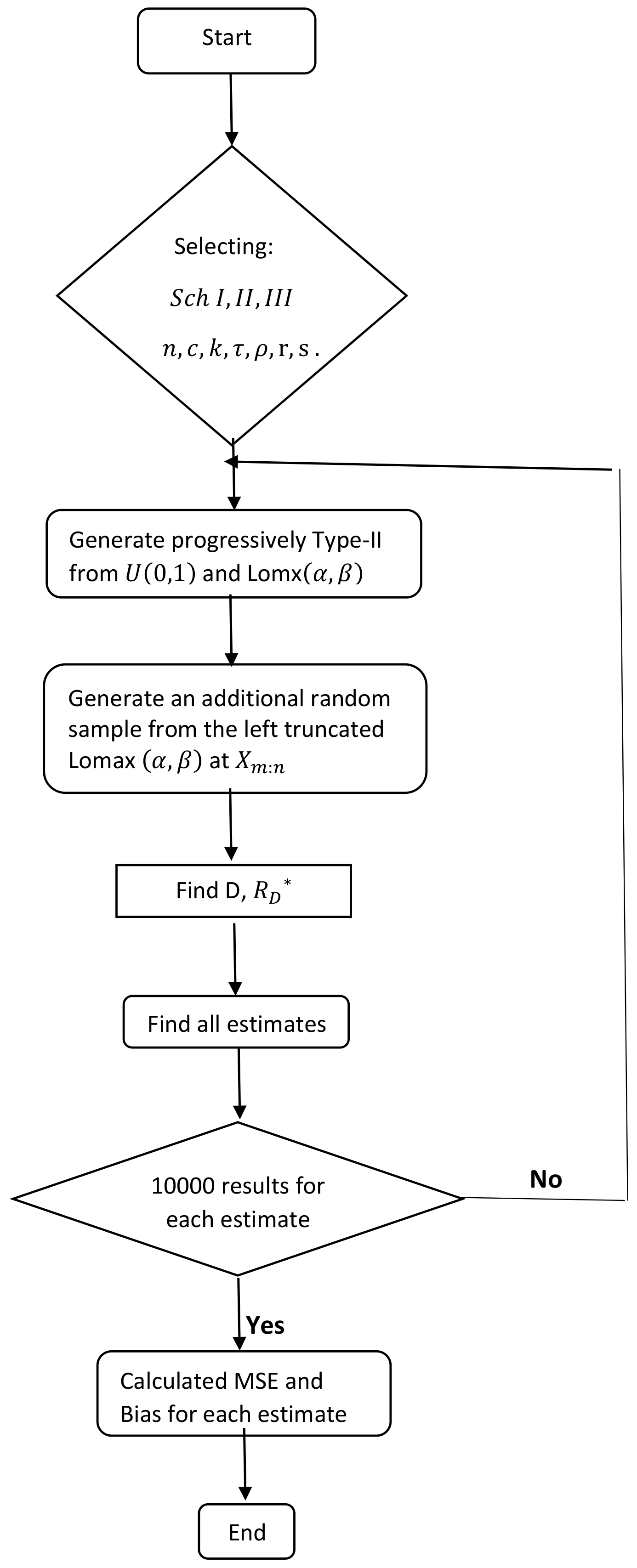
Given one of aforementioned progressive type-II censoring schemes with a combination of parameters addressed above, the simulation study was conducted according to the following steps:
  • Generate a conventional progressively type-II censored sample from Lomax( α , β ) via the transformation, x i : n = ( 1 u i : n ) 1 α 1 β , i = 1 , 2 , , m , where u 1 : n , u 2 : n , , u m : n are a conventional progressively type-II censored sample from uniform over ( 0 , 1 ) interval by using the technique of Balakrishnan and Sandhu [32].
  • Generate an additional random sample of size ( n m i = 1 m 1 R i ) from the left truncated Lomax ( α , β ) at x m : n by using the transformation x = 1 u 1 α 1 + β x m : n 1 β , where u is the uniform over ( 0 , 1 ) random variable.
  • Determine the values of D and R D , where D is the number of failures just right before time τ .
  • MLEs, c ^ and k ^ are computed simultaneously through Equations (57) and (58) for the empirical Bayesian estimations.
  • MLEs, α ^ ML , R ^ ML and h ^ ML , are computed through Equation (8) and plug-in method, respectively.
  • Under the SEL function, the Bayesian estimates, E-Bayesian estimates and empirical Bayesian estimates are computed by using Equations developed from Section 3, Section 4 and Section 5.
  • Under the LINEX loss function, the Bayesian estimates, E-Bayesian estimates and empirical Bayesian estimates are computed by using Equations developed from Section 3, Section 4 and Section 5.
  • Under the GE loss function, the Bayesian estimates, E-Bayesian estimates and empirical Bayesian estimates are computed by using Equations developed from Section 3, Section 4 and Section 5.
  • Repeat Steps 1–8 10,000 times to obtain 10,000 MLEs as well as Bayesian, empirical Bayesian and E-Bayesian estimates. Then MSEs and biases are respectively calculated based on these 10,000 values for all estimates, respectively.
The entire simulation procedure has been shown in Figure 1.
All computations were performed using Mathcad program and the computational results are displayed in Table 1 and Table 2 that display the following:
(1)
The bias and MSE of each estimate decrease as n increases.
(2)
The bias and MSE of each estimate in case of LINEX (Bayesian, empirical Bayesian and E-Bayesian) except for MSEs of the α and failure rate, h, functions decrease as b increases.
(3)
The bias and MSE of each estimate in case of GE loss function (Bayesian, empirical Bayesian and E-Bayesian) except for MSEs of the α and failure rate, h, functions decrease as P decrease.
(4)
The Bayesian estimates of α , R and h have the smallest MSE comparing among MLE, Bayesian and Emirical Bayesian estimtes.
(5)
The E-Bayesian estimates of α and failure rate, h, perform better than MLE in terms of MSE.
(6)
The E-Bayesian estimates of α and h under LINEX loss (with b = 0.5 ) perform better than the E-Bayesian estimates of α and h under LINEX loss with ( b = 1.5 ).
(7)
The E-Bayesian estimates for α and h are always underestimated (with negetive bias). The E-Bayesian estimates for R are always overestimated (with positive bias). And simulation study results are consistent with mathematical propositions for comparisons.
(8)
The E-Bayesian estimates of the square error in case first prior except for MSEs of the α and failure rate, h, functions perform better than the E-Bayesian estimates of the another square error (in case two and third priors).
(9)
The E-Bayesian estimates of GE Loss Function (p decrease) in case first prior except for MSEs of the α and failure rate, h, functions perform better than the E-Bayesian estimates of the another GE Loss Function (in case two and third priors).
(10)
The E-Bayesian estimates of α and h under GE Loss have the smallest bias comparing with all other estimates.
Overall, the Bayesian and E-Bayesian procedures with SEL, LINEX loss or GE loss can provide reliable estimates of the parameter α , R and h using the adaptive type-I progressively hybrid censored sample from Lomax( α , β ). Therefore, it is suggested to use Bayesian or E-Bayesian estimates for Lomax( α , β ) under AT-IP HCS. We do not suggest use MLE and empirical Bayesian because the results from MLE have higher MLE generally. Additionally, MLE and empirical Bayesian estimation methods are sensitive to the censoring rate and cannot always produce stable results because they are dependent upon the iterative process using quasi-Newton methods with box constraints to find MLE.

8. Applications

In this section, one simulated data set and two real data sets will be used for the illustration of Lomax ( α , β ) modeling and the applications of all estimation methods developed. For easy reference, all three complete data sets are reported in Appendix A. The first data set, which is random sample generated from Lomax ( 10.73 , 0.035 ) , is displayed in Table A1. The second data set, which was originally used by Lawless [33], consists of 60 failures is shown in Table A3. The third one comprises the 128 remission times (in months) of bladder cancer patients that was initially published by Lee and Wang [34] and is displayed in Table A5. The third data set was also used by Okasha et al. [21] for Weibull distribution modeling. However, they also mentioned that the pattern of hazard rate function revealed from data set could not be decreasing. Hence, through the intuitive guess, this data set may also be goodness-of-fitted with the Lomax distribution.
First, the Kolmogorov-Smirnov (K-S) test and scaled total time on test (TTT) plot discussed in Aarset [35] are utilized to exam the three data sets for modeling investigation. Since K-S test has been well-known and can be conducted through current existing software, we only briefly address the scaled TTT transform in this section. The scaled TTT transform is defined by T ( x ) = H 1 ( x ) / H 1 ( 1 ) with H 1 ( x ) = 0 x R ( w ) d w and 0 x 1 . Given the order statistic, X ( 1 ) < X ( 2 ) < < X ( n ) , of random sample, X i , i = 1 , 2 , , n , the empirical scaled TTT transform is derived via y ( r / n ) = H n 1 ( r / n ) / H n 1 ( 1 ) with H n 1 ( r / n ) = i = 1 r X ( i ) + ( n r ) X ( r ) and H n 1 ( 1 ) = i = 1 n X ( i ) . Then the empirical scaled TTT plot is defined as ( x , y ( x ) ) | 0 x 1 . Aarset [35] declared if the hazard increases (decreases) then the scaled TTT transform is concave (convex); moreover if the scaled TTT transform has both convex and concave joint together then the shape of hazard function is either bathtub or unimodal. The simulated data set used for Example 1 and all adaptive type-I progressively hybrid censored samples used for all examples were generated by using R that is available from author on request.

8.1. Example 1

The complete data set from Table A1 is used to fit with Lomax ( α , β ) and the MLE of the unknown α and β are obtained as α ^ = 10.69 and β ^ = 0.0347 based on the complete data set. The K-S test produces test statistic value 0.077293 with 
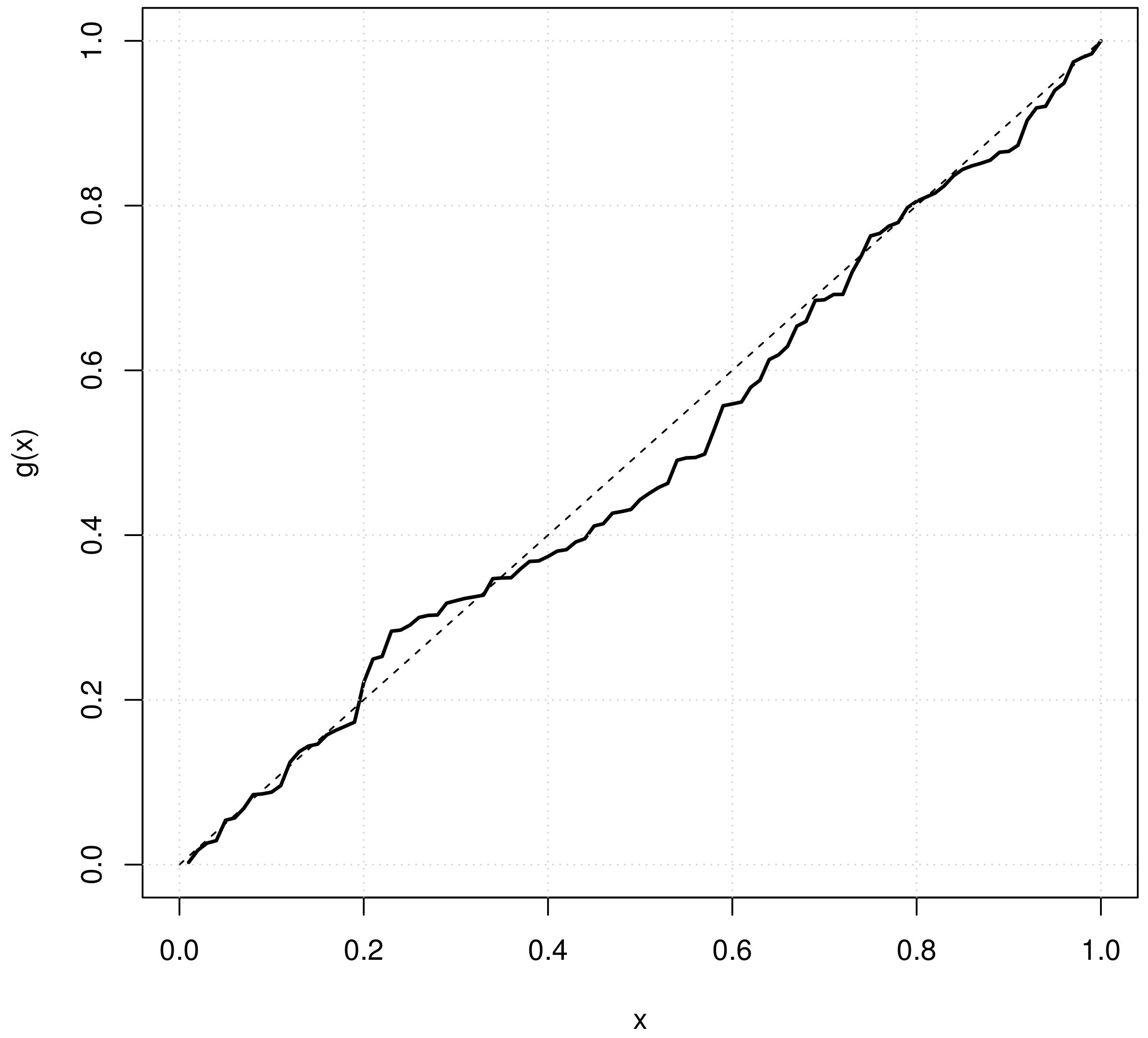
p-value = 0.5887. The empirical scaled TTT plot of the complete data from Table A1 is displayed in Figure 2 that reveals slightly convex in the small middle region of data set, concave over the small region just to the left side of the middle region and no significant pattern on both the left lower corner and the right upper corner. The pattern of TTT plot seems consistent with the pattern of hazard function that shows slightly decreasing because β is small, (for example, below 0.5). Based on p-value, the Lomax(10.69, 0.0347) is accepted to be a goodness-of-fit model.
By utilizing progressive censoring scheme II with n = 100 and m = 10 that was defined in Section 7, two adaptive type-I progressively hybrid censored samples with τ = 4 and with τ = 8 are, respectively, generated from Table A1 and displayed in Table A2. The first adaptive type-I progressively hybrid censored sample has D = 65 , R D = 26 under R i = 1 for i = 1 , 2 , , 9 and R i = 0 for i = 10 , 11 , 12 , , 65 . The second adaptive type-I progressively hybrid censored sample has D = 85 , R D = 6 under R i = 1 for i = 1 , 2 , , 9 and R i = 0 for i = 10 , 11 , 12 , , 85 . To derive the estimates of α , R ( x ) and h ( x ) , we assumed β = 0.0347 . All estimation results for α , R ( 0.4 ) and h ( 0.4 ) are calculated and displaced in Table 3 and Table 4, where Bayesian estimates were evaluated by utilizing c = 0.5 , k = 0.7 , since there are no other information available.

8.2. Example 2

The complete data set from Table A3 is used to fit with Lomax ( α , β ) and the MLE of the unknown α and β are obtained as α ^ = 11.61 and β ^ = 0.0418 based on the complete data set. The K-S test generates the test statistic 0.087169 with 
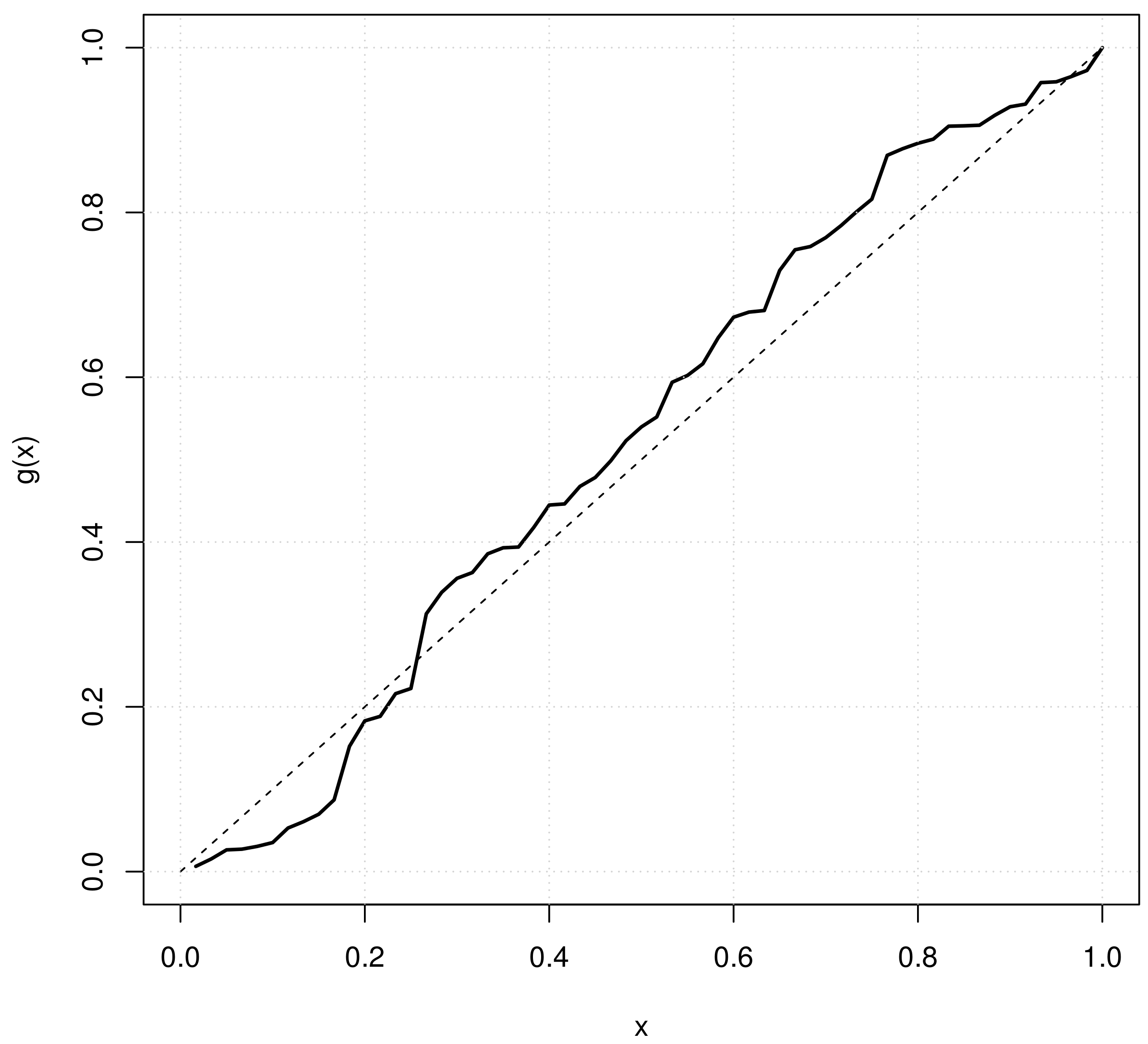
p-value = 0.719. The empirical scaled TTT plot by using the complete data from Table A3 is shown in Figure 3, which reveals slightly convex in the most left lower small corner and slightly concave with no significant pattern climbing up to the most right upper corner. The pattern of TTT plot seems consistent with the pattern of hazard function that shows slightly decreasing because β is small (for example, below 0.5). Based on p-value, the Lomax(11.61, 0.0418) is accepted to be a goodness-of-fit model.
From Table A3, two adaptive type-I progressively hybrid censored samples with τ = 4.5 and with τ = 2.0 were, respectively, generated through progressive censoring scheme II with n = 60 and m = 10 that was defined in Section 7 and displayed in Table A4. The first adaptive type-I progressively hybrid censored sample has D = 45 , R D = 6 under R i = 1 for i = 1 , 2 , , 9 and R i = 0 for i = 10 , 11 , 12 , , 45 . The second adaptive type-I progressively hybrid censored sample has D = 29 , R D = 22 under R i = 1 for i = 1 , 2 , , 9 and R i = 0 for i = 10 , 11 , 12 , , 29 . The estimates of α , R ( 0.4 ) and h ( 0.4 ) are derived assuming the true rate parameter β = 0.0418 . All estimation results for α , R ( 0.4 ) and h ( 0.4 ) are calculated and displaced in Table 3 and Table 4, where Bayesian estimates were evaluated by using c = 0.5 , k = 0.7 , since there are no other information available.

8.3. Example 3

The complete data set from Table A5 is used to fit with Lomax ( α , β ) and the MLE of unknown α and β are obtained as α ^ = 13.9384 and β ^ = 0.00826 based on the complete data set. The K-S test has test statistic value 0.096605 with p-value = 0.1833. The TTT plot of this data set had been discussed by Okasha et al. [21]. Based on p-value, there is no significant different from Lomax (13.9384, 0.00826) model fitting.
In this example, two adaptive type-I progressively hybrid censored samples with τ = 20 and with τ = 10 were respectively generated via progressive censoring scheme II with n = 128 and m = 10 that was defined in Section 7 and displayed in Table A6. The first adaptive type-I progressively hybrid censored sample has D = 106 , R D = 13 under R i = 1 for i = 1 , 2 , , 9 and R i = 0 for i = 10 , 11 , 12 , , 106 . The second adaptive type-I progressively hybrid censored sample has D = 82 , R D = 37 under R i = 1 for i = 1 , 2 , , 9 and R i = 0 for i = 10 , 11 , 12 , , 82 . The estimates of α , R ( 0.4 ) and h ( 0.4 ) are derived by utilizing β = 0.00826 . All estimation results for α , R ( 0.4 ) and h ( 0.4 ) are calculated and displaced in Table 3 and Table 4, where Bayesian estimates were computed with c = 0.5 , k = 0.7 , since there are no other information available.

9. Concluding Remarks

Based on adaptive type-I progressively hybrid censored sample, Bayesian estimations for any function of Lomax distribution shape parameter have been established. The selection of hyper-parameters in the prior and a loss function is required. For comparison purposes, the E-Bayesian and empirical Bayesian methods for any function of Lomax( α , β ) shape have been developed by utilizing the SEL, GE loss and LINEX loss functions. Three different flexible priors have also been proposed to investigate the influence of hyper-parameters on the E-Bayesian estimates of three special functions. The developed theoretical propositions for comparisons among three E-Bayesian estimates of each particular function under each loss function have also been verified by using calculated bias from the simulation study. The novel concepts and procedures provided are very useful knowledge for the future study in reliability characteristics. We have provided suggestions of the usages of all methods based on the performance comparison via an intensive simulation study and three data sets to demonstrate modeling and application illustrations. The simulation results show Bayesian estimation methods provide reliable results. However, the MLE and empirical methods are more sensitive to censoring rate.
The E-Bayesian estimates utilizing the GE and LINEX loss functions for the reliability characteristics of other lifetime distributions under the AT-IP HCS are interesting and difficult future work that are currently studied by authors.

Author Contributions

Investigation, H.O., Y.L. and M.A.; methodology, H.O., Y.L. and M.A.; software, H.O., Y.L. and M.A.; validation, H.O., Y.L. and M.A.; writing, H.O., Y.L. and M.A. All authors have read and agreed to the published version of the manuscript.

Funding

This research was funded by the Deanship of Scientific Research at King Abdel-Aziz University through the Fast-track Research Funding Program.

Institutional Review Board Statement

Not applicable.

Informed Consent Statement

Not applicable.

Data Availability Statement

Three data sets used for application have been displaced in three tables of Appendix A. The data set regarding the number of 1000s of cycles to failure for electrical appliances is also available in Lawless [33]. The 128 remission times (in months) of bladder cancer patients is also available in Lee and Wang [34].

Acknowledgments

This project was funded by the Deanship Scientific Research (DSR), King Abdulaziz University, Jeddah under grant no. (G-110-130-1442). The authors, therefore, acknowledge with thanks DSR for technical and Financial support. Authors would also like to thank the Editors and reviewers for their valuable comments and suggestions which improve this paper significantly.

Conflicts of Interest

The authors declare no conflict of interest.

Appendix A. Data Sets for Applications

Table A1. Complete data set generated from Lomax ( 10.73 , 0.035 ) .
1.6445.8305.6781.1150.5040.5240.4340.8516.0959.409
1.3323.2601.6331.7730.3910.5595.0171.4462.2691.144
5.7451.39912.5031.8463.5533.0481.2370.4650.9674.836
1.3294.4290.0780.2972.6471.2320.2090.45711.8573.617
0.0873.5460.9950.8393.3118.8983.9024.1194.9442.713
1.5481.1270.2642.9137.8620.2615.0947.9452.0210.541
5.4491.3581.4671.1030.7341.0322.5124.3932.4783.618
2.0431.0445.5940.05217.1191.7280.2716.0651.2861.042
1.2361.1351.39011.3012.0404.5387.3031.6585.2391.563
2.4944.5940.1632.9592.0710.0080.9720.1726.3121.815
Table A2. The generated censored samples using data from Table A1.
Sample I: τ = 4
0.0080.0520.0780.0870.1630.1720.2090.2610.2640.2710.2970.434
0.4570.4650.5240.5410.5590.7340.8390.8510.9670.9720.9951.032
1.0421.1031.1151.1271.1351.1441.2321.2361.2861.3291.3321.358
1.3901.3991.4461.5481.5631.6331.6441.6581.7281.8151.8462.021
2.0402.0432.0712.2692.4782.5122.6472.7132.9132.9593.0483.260
3.3113.5463.5533.6183.902
Sample II: τ = 8
0.0080.0520.0780.0870.1630.1720.2090.2610.2640.2710.2970.391
0.4340.4650.5040.5240.5590.7340.8510.9670.9720.9951.0321.044
1.1151.1271.1351.1441.2321.2361.3291.3321.3581.3901.3991.446
1.4671.5481.5631.6331.6441.6581.7281.7731.8151.8462.0212.040
2.0712.2692.4782.4942.6472.7132.9132.9593.0483.2603.3113.546
3.5533.6173.6183.9024.1194.3934.4294.5384.5944.8364.9445.017
5.0945.2395.4495.5945.6785.7455.8306.0656.0956.3127.3037.862
7.945
Table A3. Complete data set of the number of 1000s of cycles to failure for electrical appliances.
0.0140.0340.0590.0610.0690.0800.1230.1420.1650.210
0.3810.4640.4790.5560.5740.8390.9170.9690.9911.064
1.0881.0911.1741.2701.2751.3551.3971.4771.5781.649
1.7021.8931.9322.0012.1612.2922.3262.3372.6282.785
2.8112.8862.9933.1223.2483.7153.7903.8573.9124.100
4.1064.1164.3154.5104.5805.2675.2995.5836.0659.701
Table A4. The generated censored samples using data from Table A3.
Sample I: τ = 4.5
0.0140.0340.0590.0610.0690.0800.1230.1420.1650.2100.3810.464
0.4790.5560.5740.8390.9170.9690.9911.0881.1741.2701.2751.355
1.3971.4771.5781.6491.7021.8932.0012.1612.2922.3262.3372.628
2.8112.8862.9933.1223.7153.7903.8574.1004.116
Sample II: τ = 2.0
0.0140.0340.0590.0610.0690.0800.1230.1420.2100.4640.4790.556
0.5740.8390.9170.9690.9911.0641.0881.0911.2701.2751.3971.477
1.5781.6491.7021.8931.932
Table A5. The remission times (in months) from 128 bladder cancer patients.
0.080.200.400.500.510.810.901.051.191.26
1.351.401.461.762.022.022.072.092.232.26
2.462.542.622.642.692.692.752.832.873.02
3.703.823.253.313.363.363.483.523.573.64
4.514.873.884.184.234.264.334.344.404.50
5.415.494.985.065.095.175.325.325.345.41
6.977.095.625.715.856.256.546.766.936.94
7.877.937.267.287.327.397.597.627.637.66
9.7410.068.268.378.538.658.669.029.229.47
12.0312.0710.3410.6610.7511.2511.6411.7911.9812.02
12.6313.1113.2913.8014.2414.7614.7714.8315.9616.62
17.1217.1417.3618.1019.1320.2821.7322.6923.6325.74
25.8226.3132.1534.2636.6643.0146.1279.05
Table A6. The generated censored samples using data from Table A5.
Sample I: τ = 20
0.080.200.400.500.510.810.901.051.191.261.351.40
1.461.762.022.022.072.092.232.262.462.542.622.64
2.692.692.752.833.023.253.313.363.483.523.573.64
3.703.823.884.184.234.264.334.344.404.504.514.87
4.985.065.095.175.325.325.345.415.495.625.716.25
6.546.766.936.946.977.097.267.287.327.397.597.63
7.667.877.938.268.378.538.669.029.229.479.7410.06
10.3410.6610.7511.7911.9812.0312.0712.6313.1113.2913.8014.24
14.7614.7714.8315.9616.6217.1217.1417.3618.1019.13
Sample II: τ = 10
0.080.200.400.500.510.810.901.051.191.261.351.40
1.461.762.022.022.072.092.232.262.462.542.622.69
2.692.752.832.873.023.253.313.363.363.483.523.57
3.643.703.824.184.264.334.344.404.504.514.874.98
5.065.095.175.325.345.415.495.625.715.856.256.54
6.766.936.947.097.267.287.327.397.597.627.667.87
7.938.268.378.538.658.669.029.229.479.74

References

  1. Lomax, K.S. Business failure: Another example of the analysis of the failure data. J. Am. Stat. Assoc. 1954, 49, 847–852. [Google Scholar] [CrossRef]
  2. Hassan, A.S.; Al-Ghamdi, A.S. Optimum step stress accelerated life testing for Lomax distribution. J. Appl. Sci. Res. 2009, 5, 2153–2164. [Google Scholar]
  3. Al-Zahrani, B.; Al-Sobhi, M. On parameters estimation of Lomax distribution under general progressive censoring. J. Qual. Reliab. Eng. 2013, 2013, 431541. [Google Scholar] [CrossRef]
  4. Burkhalter, R.; Lio, Y. Bootstrap control charts for the generalized Pareto distribution percentiles. Chil. J. Stat. 2021, 12, 3–21. [Google Scholar]
  5. Epstein, B. Truncated life tests in the exponential case. Ann. Math. Stat. 1954, 25, 555–564. [Google Scholar] [CrossRef]
  6. Childs, A.; Chrasekar, B.; Balakrishnan, N.; Kundu, D. Exact likelihood inference based on Type-I and Type-II hybrid censored samples from the exponential distribution. Ann. Inst. Stat. Math. 2003, 55, 319–330. [Google Scholar] [CrossRef]
  7. Balakrishnan, N.; Aggarwala, R. Progressive Censoring: Theory, Methods and Applications; Birkhauser Publishers: Boston, MA, USA, 2000. [Google Scholar]
  8. Balakrishnan, N.; Cramer, E. The Art of Progressive Censoring: Applications to Reliability and Quality; Statistics for Industry and Technology; Springer: New York, NY, USA; Heidelberg, Germany; Dordrecht, The Netherlands; London, UK, 2014. [Google Scholar]
  9. Kundu, D.; Joarder, A. Analysis of Type-II progressively hybrid censored data. Comput. Stat. Data Anal. 2006, 50, 2509–2528. [Google Scholar] [CrossRef]
  10. Childs, A.; Chandrasekar, B.; Balakrishnan, N. Exact Likelihood Inference for an Exponential Parameter under Progressive Hybrid Censoring Schemes. In Statistical Models and Methods for Biomedical and Technical Systems; Birkhauser: Boston, MA, USA, 2008; pp. 319–330. [Google Scholar]
  11. Ng, H.K.T.; Kundu, D.; Chan, P.S. Statistical analysis of exponential lifetimes under an adaptive Type-II progressive censoring scheme. Naval Res. Logist. 2009, 56, 687–698. [Google Scholar] [CrossRef] [Green Version]
  12. Balakrishnan, N.; Kundu, D. Hybrid censoring: Inferential results and applications. Comput. Stat. Data Anal. 2013, 57, 166–209. [Google Scholar] [CrossRef]
  13. Lin, C.T.; Huang, Y.L. On progressive hybrid censored exponential distribution. J. Stat. Comput. Simulation. 2012, 82, 689–709. [Google Scholar] [CrossRef]
  14. Han, M. The structure of hierarchical prior distribution and its applications. Chin. Oper. Res. Manag. Sci. 1997, 6, 31–40. [Google Scholar]
  15. Han, M. E-Bayesian estimation and hierarchical Bayesian estimation of failure rate. Appl. Math. Model. 2009, 33, 1915–1922. [Google Scholar] [CrossRef]
  16. Jaheen, Z.F.; Okasha, H.M. E-Bayesian estimation for the Burr type XII model based on type-2 censoring. Appl. Math. Model. 2011, 35, 4730–4737. [Google Scholar] [CrossRef]
  17. Okasha, H.M. E-Bayesian Estimation of System Reliability with Weibull Distribution Based on Type-2 Censoring. J. Adv. Res. Sci. Comput. 2012, 4, 33–45. [Google Scholar]
  18. Okasha, H.M. E-Bayesian estimation for the Lomax distribution based on type-II censored data. J. Egypt. Math. Soc. 2014, 22, 489–495. [Google Scholar] [CrossRef] [Green Version]
  19. Ahmadi, J.; Mohammad, J.J.; March, E.; Parsian, A. Bayes estimation based on k-record data from a general class of distributions under balanced type loss functions. J. Stat. Plan. Inference 2009, 139, 1180–1189. [Google Scholar] [CrossRef]
  20. Okasha, H.M.; Mustafa, A. E-Bayesian Estimation for the Weibull Distribution under Adaptive Type-I Progressive Hybrid Censored Competing Risks Data. Entropy 2020, 22, 903. [Google Scholar] [CrossRef]
  21. Okasha, H.M.; Mohammed, H.S.; Lio, Y. E-Bayesian estimation of reliability characteristics of a Weibull distribution with applications. J. Math. 2021, 911, 1261. [Google Scholar] [CrossRef]
  22. Chiang, J.Y.; Lio, Y.L.; Tsia, T.Z. Empirical Bayesian strategy for sampling plans with warranty under truncated censoring. Int. J. Reliab. Qual. Saf. Eng. 2016, 23, 1650021. [Google Scholar] [CrossRef]
  23. Mohammed, H.S. Empirical E-Bayesian estimation for the parameter of Poisson distribution. AIMS Math. 2021, 6, 8205–8220. [Google Scholar] [CrossRef]
  24. Jaheen, Z.F. Empirical Bayes analysis of record statistics based on Linex and quadratic loss functions. Comput. Math. Appl. 2004, 47, 947–954. [Google Scholar] [CrossRef] [Green Version]
  25. Calabria, R.; Pulcini, G. Point estimation under asymmetric loss functions for left-truncated exponential samples. Commun.-Stat.-Theory Method 1996, 25, 585–600. [Google Scholar] [CrossRef]
  26. Pandey, M.; Singh, V.P.; Srivastava, C.P. Bayesian estimation of reliability model using the LINEX loss function. Microelectron. Reliab. 1994, 34, 1519–1523. [Google Scholar] [CrossRef]
  27. Soliman, A.A. Estimation of parameters of life from progressively censored data using Burr XII model. IEEE Trans. Reliab. 2005, 54, 34–42. [Google Scholar] [CrossRef]
  28. Okasha, H.; Nassar, M.; Dobbah, S.A. E-Bayesian estimation of Burr Type XII model based on adaptive Type-II progressive hybrid censored data. AIMS Math. 2021, 6, 4173–4196. [Google Scholar] [CrossRef]
  29. Nassar, M.; Okasha, H.; Albassam, M. E-Bayesian estimation and associated properties of simple step–stress model for exponential distribution based on type-II censoring. Qual. Reliab. Eng. Int. 2021, 37, 997–1016. [Google Scholar] [CrossRef]
  30. Gradshteyn, I.S.; Ryzhik, I.M. Tables of Integrals, Series and Products (Corrected and Enlarged Edition); Academic Press: San Diego, CA, USA, 1980; pp. 96–99. [Google Scholar]
  31. Yan, S.; Gendai, G. Bayes estimation for reliability indexes of cold standby system. J. North China Electr. Power Univ. 2003, 30, 96–99. [Google Scholar]
  32. Balakrishnan, N.; Sandhu, R.A. A simple simulational algorithm for generating progressive Type-II censored samples. Am. Stat. 1995, 49, 229–230. [Google Scholar]
  33. Lawless, J.F. Statistical Models and Methods for Lifetime Data; Wiley: NewYork, NY, USA, 2003. [Google Scholar]
  34. Lee, E.T.; Wang, J. Statistical Methods for Survival Data Analysis; John Wiley and Sons: Hoboken, NJ, USA, 2003. [Google Scholar]
  35. Aarset, M.V. How to identify bathtub hazard rate. IEEE Trans. Reliab. 1987, 36, 106–108. [Google Scholar] [CrossRef]
Figure 1. The flowchart for using the proposed E-Bayesian estimation methods in Section 7.
Mathematics 09 02903 g001
Figure 2. The empirical scaled TTT plot of the simulated data in Table A1.
Mathematics 09 02903 g002
Figure 3. The empirical scaled TTT plot of the failure times in Table A3.
Mathematics 09 02903 g003
Table 1. Simulated biases (first row) and MSEs (second row) under different settings with α = 3.0 , β = 1.5 , τ = 0.5 and ω = 1.5 .
BayesianEmpirical Bayesian
( n , m ) SchPar MLE LINEXSquareGeneralLINEXSquareGeneral
b = 0.5 b = 1.5 p = 1.5 p = 1.5 b = 0.5 b = 1.5 p = 1.5 p = 1.5
(20,5)I α 0.1206−0.1348−0.3424−0.0132−0.22200.02791.57691.49971.61971.64641.4836
0.66850.44040.44850.48510.49290.49412.11292.32841.9991.92662.3895
R0.00220.02520.02190.0268−0.00620.03300.47860.47470.48060.48480.458
0.00720.00660.00630.00670.00630.00700.02020.01920.02070.02170.0157
h0.1131−0.1196−0.3043−0.0124−0.20810.02621.48081.41241.51841.54351.3909
0.58760.38850.39000.42630.43320.43430.09750.11310.09320.08920.1328
II α 0.1362−0.1707−0.4117−0.0254−0.27800.02431.78751.68431.84571.87781.6825
0.85440.48720.51350.54210.56170.55381.78751.68431.84571.87781.6825
R0.00430.03040.02640.0324−0.00760.03970.43570.43130.43790.4430.4102
0.00880.00770.00740.00790.00730.00840.0220.02090.02260.02390.0166
h0.1276−0.1521−0.3669−0.0238−0.26060.02281.6791.58751.73041.76041.5773
0.75100.42970.44460.47640.49370.48670.15090.17050.1480.14420.196
III α 0.3609−0.2811−0.6381−0.0380−0.47370.04661.55511.44411.61981.66011.4121
2.15380.67320.77830.80700.86410.84272.44842.72712.32.19342.903
R−0.00020.04690.04040.0503−0.01780.06220.49650.49080.49930.50530.4663
0.01500.01180.01090.01220.01130.01330.0290.02770.02970.03080.0248
h0.3383−0.2508−0.5718−0.0356−0.44410.04371.46151.36281.51851.55641.3239
1.89300.59420.66590.70930.75950.74070.3190.28590.3490.35640.3585
(30,10)I α 0.0730−0.0890−0.2406−0.0043−0.14810.02421.35811.31121.38331.40171.2902
0.41070.30860.31070.33060.33300.33522.74692.89932.6672.60812.9758
R0.00200.01690.01470.0181−0.00480.02240.52930.52640.53080.53360.516
0.00480.00440.00430.00450.00430.00460.01870.0180.01910.01980.0157
h0.0684−0.0786−0.2130−0.0040−0.13890.02271.27471.23321.29691.31411.2095
0.36100.27200.27110.29060.29270.29460.06360.07320.05980.05640.0863
II α 0.1073−0.1154−0.3136−0.0004−0.19660.03831.36331.30191.3971.42131.2733
0.60340.40520.40830.44740.44790.45672.77462.96922.67132.59473.0798
R0.00240.02210.01910.0237−0.00730.02950.52990.5260.53180.53540.5122
0.00660.00600.00580.00610.00590.00640.0210.02010.02150.02240.0172
h0.1006−0.1018−0.2780−0.0004−0.18430.03591.281.22571.30971.33251.1937
0.53030.35750.35540.39320.39370.40140.10210.1110.09990.09640.1341
III α 0.2616−0.1574−0.44040.0202−0.28360.07971.40341.31941.45111.48441.2807
1.25860.52750.53870.63200.61140.65892.58152.85052.43552.33492.9857
R−0.00350.02910.02460.0315−0.01590.04000.51570.51050.51820.52330.4903
0.01000.00790.00750.00810.00820.00860.01650.01530.01720.01840.0114
h0.2452−0.1380−0.39100.0189−0.26580.07471.31831.24371.36041.36041.2007
1.10620.46680.46570.55550.53740.57910.04590.06570.04010.03670.0884
(45,15)I α 0.0477−0.0541−0.16210.0042−0.09390.02371.32191.29031.33861.35111.2755
0.26780.22340.22170.23510.23440.23752.85532.96052.80092.75973.0139
R0.00140.01110.00960.0119−0.00380.01490.53830.53630.53930.54120.5294
0.00320.00310.00300.00310.00310.00320.01850.0180.01880.01930.0165
h0.0447−0.0474−0.14290.0039−0.08810.02221.24031.21231.25491.26661.1958
0.23540.19680.19400.20660.20610.20880.05540.06250.05230.04960.0707
II α 0.0812−0.0765−0.22180.0043−0.13220.03131.28631.24531.30821.32511.223
0.40160.29470.29290.31700.31540.32182.99783.13552.92582.86943.22
R0.00070.01520.01300.0162−0.00550.02040.54820.54540.54950.55210.5363
0.00460.00410.00400.00420.00410.00430.01960.01890.02000.02060.0169
h0.0761−0.0671−0.19600.0040−0.12390.02941.20721.17101.22651.24231.1466
0.35300.25980.25580.27860.27720.28280.07350.08120.07060.06730.0949
III α 0.1627−0.1006−0.32090.0298−0.18950.07301.40011.33951.43331.45661.3148
0.73860.41980.40840.48600.46230.50252.58812.78162.48552.41372.867
R−0.00170.02030.01710.0220−0.01230.02840.51720.51350.5190.52260.4998
0.00700.00590.00560.00600.00610.00620.01770.01680.01820.01910.0138
h0.1526−0.0871−0.28330.0279−0.17770.06841.31451.26081.34381.36561.2327
0.64910.37130.35560.42710.40630.44160.04870.06450.04260.03840.0792
Table 2. Simulated biases (first row) and MSEs (second row) under different settings with α = 3.0 , β = 1.5 , τ = 0.5 and ω = 1.5 .
E-Bayesian
( n , m ) SchParLINEXSquareGeneral
b = 0.5 b = 1.5 p = 1.5 p = 1.5
EBL1EBL2EBL3EBL1EBL2EBL3EBS1EBS2EBS3EBG1EBG2EBG3EBG1EBG2EBG3
(20,5)I α −0.3241−0.2143−0.4339−0.5180−0.4235−0.6126−0.2105−0.0910−0.3300−0.1557−0.0337−0.2778−0.4053−0.2938−0.5167
0.47610.46850.51130.56040.50830.63260.46960.49600.47620.46210.50340.45510.55650.53540.6065
R0.05000.03620.06370.04640.03270.06010.05180.03800.06560.05640.04280.07000.01650.00180.0312
0.00880.00770.01020.00830.00740.00960.00900.00790.01050.00950.00830.01100.00690.00680.0075
h−0.2975−0.1941−0.4009−0.4701−0.3802−0.5599−0.1973−0.0853−0.3093−0.1460−0.0316−0.2604−0.3800−0.2755−0.4844
0.41730.41220.44690.48300.44010.54420.41280.43600.41860.40610.44240.40000.48910.47050.5331
II α −0.3750−0.2444−0.5056−0.6003−0.4909−0.7096−0.2376−0.0929−0.3824−0.1828−0.0350−0.3305−0.4857−0.3537−0.6178
0.56520.55750.61300.67840.60820.77620.55940.60480.56410.55130.61510.53970.68640.65730.7575
R0.05860.04210.07510.05430.03780.07070.06070.04410.07720.06760.05120.08390.01940.00150.0372
0.01080.00940.01280.01020.00890.01200.01110.00960.01310.01200.01030.01420.00840.00820.0092
h−0.3440−0.2208−0.4672−0.5450−0.4409−0.6491−0.2228−0.0871−0.3585−0.1713−0.0328−0.3099−0.4554−0.3315−0.5792
0.49530.49090.53540.58360.52590.66660.49170.53150.49580.48460.54070.47430.60330.57770.6658
III α −0.6083−0.4046−0.8120−0.9301−0.7767−1.0835−0.3744−0.1267−0.6220−0.2777−0.0212−0.5343−0.8073−0.6000−1.0147
0.88610.84641.03331.18361.00791.41710.88831.04370.90210.84381.05500.81251.21701.13001.4234
R0.09730.06980.12490.08970.06230.11700.10070.07310.12830.11080.08380.13780.15300.16220.1576
0.02010.01640.02540.01840.01500.02330.02110.01720.02650.02260.01830.02850.03150.03770.0628
h−0.5586−0.3656−0.7516−0.8483−0.7011−0.9954−0.3510−0.1188−0.5832−0.2604−0.0198−0.5009−0.7569−0.5625−0.9513
0.77400.74580.89891.01060.86241.21230.78070.91730.79280.74170.92720.71411.06960.99321.2510
(30,10)I α −0.2176−0.1384−0.2968−0.3626−0.2914−0.4338−0.1380−0.0543−0.2218−0.1056−0.0208−0.1904−0.2776−0.1978−0.3574
0.33570.33500.35020.37430.34940.41020.32530.33950.32670.32290.34300.31860.36630.35670.3900
R0.03350.02390.04310.03110.02150.04060.03450.02490.04420.03860.02900.04810.01090.00090.0210
0.00560.00510.00630.00540.00490.00600.00550.00500.00620.00580.00530.00660.00470.00460.0049
h−0.1994−0.1249−0.2739−0.3280−0.2606−0.3954−0.1294−0.0509−0.2079−0.0990−0.0195−0.1785−0.2603−0.1854−0.3351
0.29460.29480.30670.32430.30410.35440.28590.29840.28710.28380.30150.28000.32200.31350.3428
II α −0.2862−0.1812−0.3912−0.4728−0.3817−0.5639−0.1851−0.0719−0.2983−0.1441−0.0291−0.2592−0.3781−0.2724−0.4838
0.44150.44080.46740.50820.46550.56970.42470.45070.42800.43950.48000.42980.51750.50200.5591
R0.04450.03150.05740.04120.02830.05400.04660.03360.05950.05260.03980.06540.01520.00150.0289
0.00780.00700.00900.00750.00670.00850.00780.00700.00910.00850.00750.00990.00640.00630.0069
h−0.2622−0.1633−0.3611−0.4282−0.3417−0.5147−0.1735−0.0674−0.2796−0.1351−0.0273−0.2430−0.3545−0.2554−0.4536
0.38730.38820.40880.43870.40390.49050.37330.39610.37620.38630.42190.37780.45480.44120.4914
III α −0.4043−0.2488−0.5599−0.6653−0.5393−0.7912−0.2568−0.0820−0.4316−0.1925−0.0136−0.3713−0.5552−0.3993−0.7110
0.60770.61070.66460.74670.65810.87310.63070.71600.62360.58980.69410.56620.75130.71380.8504
R0.06350.04390.08300.05840.03900.07780.06840.04890.08800.07570.05650.09500.0184−0.00300.0398
0.01160.01000.01410.01090.00940.01310.01250.01070.01510.01300.01090.01580.00880.00890.0096
h−0.3701−0.2232−0.5170−0.6035−0.4833−0.7237−0.2407−0.0769−0.4046−0.1804−0.01280.0950−0.5205−0.3743−0.6666
0.53270.53910.57980.64020.56740.74760.55430.62930.54810.51840.61000.49760.66030.62740.7474
(45,15)I α −0.1516−0.0962−0.2070−0.2558−0.2043−0.3072−0.0936−0.0360−0.1513−0.0719−0.0137−0.1300−0.1892−0.1333−0.2450
0.22980.22940.23680.24890.23650.26690.25900.23610.22910.22750.23720.22500.24730.24320.2582
R0.02300.01640.02960.02140.01480.02790.02360.01700.03020.02640.01980.03290.00750.00070.0143
0.00360.00330.00390.00350.00330.00380.00360.00340.00390.00380.00350.00410.00320.00320.0033
h−0.1389−0.0868−0.1910−0.2310−0.1825−0.2795−0.0878−0.0337−0.1419−0.0674−0.0129−0.1219−0.1773−0.1250−0.2297
0.20180.20180.20760.21640.20640.23140.20130.20750.20130.20000.20850.19780.21740.21380.2269
II α −0.1988−0.1230−0.2746−0.3381−0.2696−0.4066−0.1267−0.0469−0.2065−0.0934−0.0126−0.1743−0.2566−0.1802−0.3329
0.31320.31430.32460.34540.32410.37700.30740.32180.30710.30750.32800.30150.34260.33600.3622
R0.03060.02150.03980.02840.01930.03750.03220.02300.04130.03570.02660.04480.00950.000040.0190
0.00510.00470.00570.00490.00460.00550.00510.00460.00570.00530.00480.00600.00430.00430.0045
h−0.1820−0.1106−0.2532−0.3055−0.2407−0.3702−0.1188−0.0440−0.1936−0.0876−0.0118−0.1634−0.2405−0.1690−0.3121
0.2700.27670.28440.29950.28230.32590.27020.28280.26990.27030.28830.26500.30110.29530.3184
III α −0.2989−0.1816−0.4161−0.5043−0.4043−0.6044−0.1756−0.0471−0.3041−0.1354−0.0051−0.2657−0.3966−0.2781−0.5151
0.45590.46300.48140.52760.47980.59870.46990.52170.45800.46370.52670.44160.53580.52450.5812
R0.04630.03200.06060.04260.02840.05690.04800.03370.06240.05480.04060.06900.0133−0.00190.0286
0.00790.00700.00920.00750.00670.00870.00820.00730.00950.00880.00770.01030.00670.00680.0071
h−0.2734−0.1629−0.3840−0.4564−0.3613−0.5515−0.1646−0.0442−0.2851−0.1269−0.0048−0.2491−0.3718−0.2607−0.4829
0.40020.40850.42100.45470.41610.51430.41300.45850.40260.40750.46290.38820.47090.46090.5108
Table 3. Different estimates of the generated adaptive type-I progressively censored samples from three examples under different settings with m = 10 and ω = 1.5 .
BayesianEmpirical Bayesian
ExampleSamplePar MLE LINEXSquareGeneralLINEXSquareGeneral
b = 0.5 b = 1.5 p = 1.5 p = 1.5 b = 0.5 b = 1.5 p = 1.5 p = 1.5
β = 0.0347 , n = 100
11 α 9.88098.70368.18248.99938.82749.03357.96647.56758.18798.04758.2158
R0.87270.88340.88330.88340.88320.88350.87190.87180.89330.89320.8934
h0.33820.30760.30690.30800.30210.30920.28000.27940.28020.27540.2812
2 α 10.09709.12868.68089.37679.23959.40409.97999.498310.24619.239510.2730
R0.87010.87880.87870.87880.87860.87890.86920.86910.86840.87860.8684
h0.34560.32060.32000.32090.31620.32190.35040.34970.35070.31620.3516
β = 0.0418 , n = 60
21 α 11.92339.64048.770210.16969.889910.225211.132910.188311.700011.440911.7516
R0.82060.84500.84480.84510.84440.84520.81880.81860.82390.82320.8241
h0.49020.41710.41450.41810.40660.42040.48000.47800.48100.47040.4831
2 α 10.44507.92837.05458.48578.12568.55717.34276.70427.72807.46087.7811
R0.84100.86890.86870.86900.86830.86920.83970.83940.87990.87940.8800
h0.42940.34780.34580.34890.33410.35180.31700.31560.31770.30670.3199
β = 0.00826 , n = 128
31 α 14.066212.554011.879712.931412.779512.961710.915610.456311.166111.189211.0504
R0.95470.95820.95820.95830.95820.95830.97490.96710.96380.96380.9638
h0.11580.10640.10640.10650.10520.10670.08070.09190.09190.09210.0910
2 α 13.784711.964111.189112.408512.220412.446110.589110.054910.885910.9140910.74438
R0.95550.95990.95990.95990.95990.95990.97950.96970.96470.96470.96472
h0.11350.10210.10210.10220.10060.10250.07640.08960.08960.089850.08846
Table 4. Cont. Table 3.
E-Bayesian
ExampleSampleParLINEXSquareGeneral
b = 0.5 b = 1.5 p = 1.5 p = 1.5
EBL1EBL2EBL3EBL1EBL2EBL3EBS1EBS2EBS3EBG1EBG2EBG3EBGEBG2EBG3
β = 0.0347 , n = 100
11 α 8.66148.94808.37478.14298.39697.88888.95569.26198.64928.78449.08498.48398.98989.29738.68226
R0.883960.880230.887690.883870.880140.887610.884010.880280.88770.88380.88010.887490.884060.88030.88778
h0.30620.31660.29570.30540.31580.29500.30650.31700.29600.30070.31090.29040.30770.31820.2972
2 α 9.08889.33068.84708.64348.86258.42449.33559.59059.08059.19909.45028.94769.36299.61869.1071
R0.87930.87620.88240.879250.876160.88230.87940.87630.88250.87920.87610.88230.87940.87630.8825
h0.31920.32790.31050.31860.32730.30990.31950.32820.310780.314830.323430.30620.32040.32920.31170
β = 0.0418 , n = 60
21 α 9.598210.10519.09128.72809.14998.306210.128610.69249.56479.849610.39799.301210.184210.75129.6173
R0.84570.83780.85360.84550.83760.85340.84580.83790.85370.84510.83720.85310.84590.83810.8538
h0.41550.43850.39240.41360.43640.39070.41640.43960.39320.40500.42750.38240.418700.44200.3954
2 α 7.90238.43277.37197.02337.44646.60028.46629.07387.85868.10588.68767.52418.53789.1505397.9251
R0.86930.86060.87810.86910.86030.87780.86950.86080.87820.86870.85990.87750.86960.86090.8783
h0.34700.37190.32220.34500.36950.32040.34810.37310.32310.33330.35720.30930.35100.37620.3258
β = 0.00826 , n = 128
31 α 12.50112.868112.133911.830112.159511.500612.876513.265912.487112.725313.110112.340512.906913.297112.5166
R0.95840.95720.95960.95840.95720.95960.95840.95720.95970.95840.95720.95970.95840.95720.9597
h0.10600.10920.10280.10590.10910.10270.1060 60.10920.10280.10480.10790.10160.10630.10950.1031
2 α 11.910012.340311.479811.138411.515910.761012.352812.815411.890212.165512.62111.709912.390312.854311.9264
R0.96010.95860.96160.96010.95860.96160.96010.95860.96160.96010.95860.96150.96010.95860.9616
h0.10170.10550.097860.10160.10540.09780.10170.10550.09790.10020.10390.09640.10200.10580.09819
Publisher’s Note: MDPI stays neutral with regard to jurisdictional claims in published maps and institutional affiliations.

