Article

Contrast-Independent, Partially-Explicit Time Discretizations for Nonlinear Multiscale Problems

1
Department of Mathematics, The Chinese University of Hong Kong, Shatin, New Territories, Hong Kong, China
2
Department of Mathematics, Institute for Scientific Computation (ISC), Texas A&M University, College Station, TX 77845, USA
3
Multiscale Model Reduction Laboratory, North-Eastern Federal University, 677980 Yakutsk, Russia
4
Department of Mathematics, University of California, Irvine, CA 92697, USA
*
Author to whom correspondence should be addressed.
Mathematics 2021, 9(23), 3000; https://doi.org/10.3390/math9233000
Submission received: 1 October 2021 / Revised: 10 November 2021 / Accepted: 11 November 2021 / Published: 23 November 2021
(This article belongs to the Special Issue Computational Mathematics, Algorithms, and Data Processing)

Abstract

:
This work continues a line of work on developing partially explicit methods for multiscale problems. In our previous works, we considered linear multiscale problems where the spatial heterogeneities are at the subgrid level and are not resolved. In these works, we have introduced contrast-independent, partially explicit time discretizations for linear equations. The contrast-independent, partially explicit time discretization divides the spatial space into two components: contrast dependent (fast) and contrast independent (slow) spaces defined via multiscale space decomposition. Following this decomposition, temporal splitting was proposed, which treats fast components implicitly and slow components explicitly. The space decomposition and temporal splitting are chosen such that they guarantees stability, and we formulated a condition for the time stepping. This condition was formulated as a condition on slow spaces. In this paper, we extend this approach to nonlinear problems. We propose a splitting approach and derive a condition that guarantees stability. This condition requires some type of contrast-independent spaces for slow components of the solution. We present numerical results and show that the proposed methods provide results similar to implicit methods with a time step that is independent of the contrast.

1. Introduction

Nonlinear problems arise in many applications, and they are typically described by some nonlinear partial differential equations. In many applications, these problems have multiscale nature and contain multiple scales and high contrast. Examples include nonlinear porous media flows (Richards’ equations, Forchheimer flow and so on; see [1,2]), where the media properties contain many spatial scales and high contrast. Due to high contrast in the media properties, these processes also occur on multiple time scales. E.g., for nonlinear diffusion, the flow can be fast in high conductivity regions and slow in low conductivity regions. Due to a disparity of time scales, special temporal discretizations are often sought, which is the main goal of the paper in the context of multiscale problems.
When the media properties are high, the flow and transport become fast and require small time steps to resolve the dynamics. Implicit discretization can be used to handle fast dynamics; however, this requires solving large-scale nonlinear systems. For nonlinear problems, explicit methods are used when possible to avoid solving nonlinear systems. The main drawback of explicit methods is that they require small time steps that scale as the fine mesh and depend on physical parameters, e.g., the contrast. To alleviate this issue, we propose a novel nonlinear splitting algorithm following our earlier works [3,4] for linear equations. The main idea of our approaches is to use multiscale methods on a coarse spatial grid such that the time step scales with the coarse mesh size.
Next, we give a brief overview of multiscale methods for spatial discretizations that are used in our paper. Multiscale spatial algorithms have been extensively studied for linear and nonlinear problems. For linear problems, many multiscale methods have been developed. These include homogenization-based approaches [5,6], multiscale finite element methods [5,7,8], generalized multiscale finite element methods (GMsFEM) [9,10], constraint energy minimizing GMsFEM (CEM-GMsFEM) [11,12], nonlocal multi-continua (NLMC) approaches [13], metric-based upscaling [14], the heterogeneous multiscale method [15], localized orthogonal decomposition (LOD) [16], equation-free approaches [17,18], multiscale stochastic approaches [19,20,21] and the hierarchical multiscale method [22]. For high-contrast problems, approaches such as GMsFEM and NLMC have been developed. For example, in the GMsFEM [11], multiple basis functions or continua were designed to capture the multiscale features due to high contrast [12,13]. These approaches require careful designing of multiscale dominant modes. For nonlinear problems, linear multiscale basis functions can be replaced by nonlinear maps [23,24,25].
Our proposed approaches follow concepts developed in [3,4] for linear equations. In these works, we designed splitting algorithms for solving flow and wave equations. In both cases, the solution space was divided into two parts, the coarse-grid part and the correction part. The coarse-grid solution is computed using multiscale basis functions with CEM-GMsFEM. The correction part uses special spaces in the complement space (the complement to the coarse space). A careful choice of these spaces guarantees that the method is stable. Our analysis in [3,4] shows that for the stability, the correction space should be free of contrast, and thus, this requires a special multiscale space construction. These splitting algorithms have their origins in earlier works [26,27]. In this paper, we extend the linear concepts to nonlinear problems.
Splitting algorithms for nonlinear problems have often been used in the literature. Earlier approaches include implicit-explicit approaches and other techniques [28,29,30,31,32,33,34,35,36,37,38,39,40]. In many approaches, nonlinear contributions are roughly divided into two parts depending on whether it is easy to implicitly solve discretized system. For easy to solve part, implicit discretization is used, and for the rest, explicit discretization is used. However, in general, one cannot separate these parts for the problems under consideration. Our goal is to use splitting concepts and treat implicitly and explicitly some parts of the solution. As a result, we can use larger time steps that scale with the coarse mesh size.
Our approach starts with a nonlinear dynamical system
u t + f ( u ) + g ( u ) = 0 ,
where f ( u ) represents diffusion-like operator, and g ( u ) represents reaction-like terms. In linear problems, for the stability, we formulate a condition that involves the time step, the energy and the L 2 norm of the solution in the complement space. This is a constraint for the time step. With an appropriate choice of the complement space, this condition guarantees stability for the time steps that scale with the coarse mesh size. To obtain similar conditions for nonlinear problems, we carried out the analysis for nonlinear f ( u ) and g ( u ) functions. The analysis revealed conditions that are required for stability. The conditions of multiscale spaces share some similarities with those for nonlinear multiscale methods [25]. We made several observations.
  • Additional degrees of freedom are needed for dynamic problems, in general, to handle missing information.
  • We note that restrictive time steps scale with the coarse mesh size, and thus, are much coarser.
We would like to note that the proposed concepts of partially explicit methods can be used in conjunction with other multiscale methods that deal with high contrast. However, multiscale approaches that do not explicitly take into account the high contrast via additional degrees of freedom (when necessary) may not benefit from our proposed concepts (cf. [15,41,42]). Due to high contrast, small time scales appear, and our goal is to find out those few degrees of freedom that are responsible for the fast dynamics and handle them separately. This condition is rigorously derived and any approaches that split spaces accordingly can be used in the framework of partially explicit methods.
We present several numerical results. In our numerical demonstrations, we consider two cases. In the first case, we took the reaction term, g ( u ) , to be nonlinear and the diffusion term, f ( u ) , to be linear. In the second case, we consider both to be nonlinear and used for f ( u ) the form f ( u ) = d i v ( κ ( x , u ) u ) . The media properties for the diffusion are taken to be heterogeneous, and we chose smooth and singular source terms. We compared the proposed approach to the approach where all degrees of freedom are handled implicitly. We show here that the proposed method provides an approximation similar to fully implicit methods.
The paper is organized as follows. In the next section, we provide some preliminaries. In Section 3, we present our main assumptions and stability estimates for a fine-grid problem. In Section 4, we describe the partially explicit method and its stability. The discussion is in Section 5. Numerical results are presented in Section 6.

2. Problem Setting

We consider the following equation:
u t = f ( u ) g ( u ) ,
where f = δ F δ u and g = δ G δ u which are the variational derivative of energies F ( u ) : = Ω E 1 ( u ) and G ( u ) : = Ω E 2 ( u ) . Here, f is assumed to be contrast dependent nonlinear (or linear) (i.e., f introduces stiffness in the system) and g is contrast independent (i.e., g does not introduce stiffness).
We assume f ( u ) V * and g ( u ) L 2 ( Ω ) for all u V . We can then consider the weak formulation of the problem, namely, finding u V such that
( u t , v ) = ( f ( u ) , v ) V * , V ( g ( u ) , v ) L 2 v V .
To simplify the notation, we simply write ( · , · ) instead of ( · , · ) V * , V in the following discussion.
Example 1. For F ( u ) = 1 2 Ω κ | u | 2 and G ( u ) = 0 , we have f ( u ) = δ F δ u H 1 ( Ω ) = ( H 1 ( Ω ) ) * for V = H 1 ( Ω ) .
( δ F δ u ( u ) , v ) = Ω κ u · v ,
and thus, we have
f ( u ) = · ( κ u ) .
In strong form, we have
u t = · ( κ u ) .
Example 2. For F = 1 p κ | u | p and G ( u ) = 0 , we have f ( u ) = δ F δ u W 1 , p p 1 ( Ω ) = ( W 1 , p ( Ω ) ) * for V = W 1 , p ( Ω )
( δ F δ u ( u ) , v ) = κ | u | p 2 u · v ,
and thus, we have
f ( u ) = · ( κ | u | p 2 u ) .
In strong form, we have
u t = · ( κ | u | p 2 u ) .
In the following discussion, we make the following assumptions about the second variational derivatives of F and G.
  • The second variational derivatives δ 2 F and δ 2 G satisfy
    δ 2 F ( u ) ( v , v ) c ( u ) v V 2 u , v V
    δ 2 G ( u ) ( v , v ) b ( u ) v 2 u , v V ,
    where 0 c ( u ) < and b ̲ b ( u ) < are independent of v.
  • The second variational derivatives δ 2 F and δ 2 G are bounded. That is,
    | δ 2 F ( u ) ( w , v ) | C ( u ) v V w V u , v , w V
    | δ 2 G ( u ) ( w , v ) | B v L 2 w L 2 u , v , w V ,
    where 0 < C ( u ) < and 0 < B < are independent on v , w .

3. Discretization

To solve the problem, a standard method is the finite element approach. We can consider that the numerical solution u H ( t , · ) V H satisfies
( u H , t , v ) = ( f ( u ) + g ( u ) , v ) v V H ,
where V H is a finite element space in V.
For the time discretization, we can consider two simplest discretizations which are forward Euler and backward Euler methods. For the forward Euler method, we consider { u H k } k = 0 N V H such that
( u H n + 1 u H n Δ t , v ) + ( f ( u H n ) + g ( u H n ) , v ) = 0 v V H .
For the backward Euler method, we consider { u H k } k = 0 N V H such that
( u H n + 1 u H n Δ t , v ) + ( f ( u H n + 1 ) + g ( u H n + 1 ) , v ) = 0 v V H .
Next, we would like to derive stability conditions for backward and forward Euler methods.
Since
F ( u H n ) = F ( u H n + 1 ) ( f ( u H n + 1 ) , u H n + 1 u H n ) + 1 2 δ 2 F ( ξ 1 n ) ( u H n + 1 u H n , u H n + 1 u H n )
and
G ( u H n ) = G ( u H n + 1 ) ( g ( u H n + 1 ) , u H n + 1 u H n ) + 1 2 δ 2 G ( ξ 2 n ) ( u H n + 1 u H n , u H n + 1 u H n )
for some ξ i n = ( 1 λ i ) u H n + 1 + λ i u H n with λ i ( 0 , 1 ) and i = 1 , 2 , we have
0 = ( u H n + 1 u H n Δ t , u H n + 1 u H n ) + ( f ( u H n + 1 ) + g ( u H n + 1 ) , u H n + 1 u H n ) = 1 Δ t u H n + 1 u H n 2 + F ( u H n + 1 ) F ( u H n ) + G ( u H n + 1 ) G ( u H n ) + 1 2 δ 2 F ( ξ 1 n ) ( u H n + 1 u H n , u H n + 1 u H n ) + 1 2 δ 2 G ( ξ 2 n ) ( u H n + 1 u H n , u H n + 1 u H n ) 1 Δ t + b ( u ) u H n + 1 u H n 2 + F ( u H n + 1 ) F ( u H n ) + G ( u H n + 1 ) G ( u H n ) + c ( u ) 2 u H n + 1 u H n V 2 .
We have
F ( u H n + 1 ) + G ( u H n + 1 ) F ( u H n + 1 ) + G ( u H n + 1 ) + c ( u ) 2 u H n + 1 u H n V 2 + 1 Δ t b ̲ u H n + 1 u H n 2 F ( u H n ) + G ( u H n )
for any Δ t , and thus, the backward Euler method is stable if Δ t b ̲ 1 .
Similarly, for the forward Euler method, we can use
F ( u H n + 1 ) = F ( u H n ) + ( f ( u H n ) , u H n + 1 u H n ) + 1 2 δ 2 F ( ξ 1 n ) ( u H n + 1 u H n , u H n + 1 u H n ) ,
G ( u H n + 1 ) = G ( u H n ) + ( g ( u H n ) , u H n + 1 u H n ) + 1 2 δ 2 G ( ξ 2 n ) ( u H n + 1 u H n , u H n + 1 u H n )
and obtain
0 = ( u H n + 1 u H n Δ t , u H n + 1 u H n ) + ( f ( u n ) + g ( u H n ) , u H n + 1 u H n ) = 1 Δ t u H n + 1 u H n 2 + F ( u H n + 1 ) F ( u H n ) + G ( u H n + 1 ) G ( u H n ) 1 2 δ 2 F ( ξ 1 n ) ( u H n + 1 u H n , u H n + 1 u H n ) 1 2 δ 2 G ( ξ 2 n ) ( u H n + 1 u H n , u H n + 1 u H n ) ( 1 Δ t B ) u H n + 1 u H n 2 + F ( u H n + 1 ) F ( u H n ) + G ( u H n + 1 ) G ( u H n ) C ( ξ n ) 2 u H n + 1 u H n V 2 .
Therefore, if Δ t C ( ξ ) 2 u H n + 1 u H n V 2 u H n + 1 u H n 2 + B 1 for any ξ = ( 1 λ ) u H k + 1 + λ u H k with 0 k N 1 , we have
F ( u H n + 1 ) + G ( u H n + 1 ) F ( u H n ) + G ( u H n ) .
We can see that although forward Euler method is easier for implementation, we require a small time step for stability if sup v V H v V 2 v 2 or C ( ξ ) is large.
We remark that in typical cases we consider values of b ̲ and B that are not too large. Therefore, Δ t b ̲ and Δ t B are small and the energy G will not affect the stability too much.

4. Partially Explicit Scheme with Space Splitting

To obtain an efficient method, one can consider partially explicit scheme by splitting finite element space. We consider that V H is a direct sum of two subspaces V H , 1 and V H , 2 , namely, V H = V H , 1 V H , 2 . The finite element solution is then satisfying
( u H , 1 , t + u H , 2 , t , v 1 ) + ( f ( u H , 1 + u H , 2 ) + g ( u H , 1 + u H , 2 ) , v 1 ) = 0 v 1 V H , 1 , ( u H , 1 , t + u H , 2 , t , v 2 ) + ( f ( u H , 1 + u H , 2 ) + g ( u H , 1 + u H , 2 ) , v 2 ) = 0 v 2 V H , 2 ,
where u H = u H , 1 + u H , 2 . We can use a partially explicit time discretization. For example, we can consider
( u H , 1 n + 1 u H , 1 n Δ t + u H , 2 n u H , 2 n 1 Δ t , v 1 ) + ( f ( u H , 1 n + 1 + u H , 2 n ) + g ( u H , 1 n + u H , 2 n ) , v 1 ) = 0 v 1 V H , 1 , ( u H , 1 n u H , 1 n 1 Δ t + u H , 2 n + 1 u H , 2 n Δ t , v 2 ) + ( f ( u H , 1 n + 1 + u H , 2 n ) + g ( u H , 1 n + u H , 2 n ) , v 2 ) = 0 v 2 V H , 2 .

Energy Stability

Lemma 1.
If
( f ( u H n + 1 ) f ( u H , 1 n + 1 + u H , 2 n ) , u H n + 1 u H n ) c ¯ 2 u H n + 1 u H n V 2 + ( 1 γ ) Δ t ( 1 + γ ) B 2 i u H , i n + 1 u H , i n 2 ,
where c ¯ = inf u V H c ( u ) and γ = sup v 1 V H , 1 , v 2 V H , 2 ( v 1 , v 2 ) v 1 v 2 < 1 [43], we have
γ 2 Δ t i u H , i n + 1 u H , i n 2 + F ( u H n + 1 ) + G ( u H n + 1 ) γ 2 Δ t i u H , i n u H , i n 1 2 + F ( u H n ) + G ( u H n ) .
Proof. 
By substituting v 1 = u H , 1 n + 1 u H , 1 n and v 2 = u H , 2 n + 1 u H , 2 n , we have
1 Δ t u H , 1 n + 1 u H , 1 n 2 + 1 Δ t ( u H , 2 n u H , 2 n 1 , u H , 1 n + 1 u H , 1 n ) + ( f ( u H , 1 n + 1 + u H , 2 n ) + g ( u H n ) , u H , 1 n + 1 u H , 1 n ) = 0 ,
and
1 Δ t u H , 2 n + 1 u H , 2 n 2 + 1 Δ t ( u H , 1 n u H , 1 n 1 , u H , 2 n + 1 u H , 2 n ) + ( f ( u H , 1 n + 1 + u H , 2 n ) + g ( u H n ) , u H , 2 n + 1 u H , 2 n ) = 0 .
Summing up the above two equations, we have
1 Δ t i u H , i n + 1 u H , i n 2 + 1 Δ t i j ( u H , i n u H , i n 1 , u H , j n + 1 u H , j n ) + ( f ( u H , 1 n + 1 + u H , 2 n ) + g ( u H n ) , u H n + 1 u H n ) = 0 .
We first use
1 Δ t | i j ( u H , i n u H , i n 1 , u H , j n + 1 u H , j n ) | γ Δ t i j u H , i n u H , i n 1 u H , j n + 1 u H , j n γ 2 Δ t i u H , i n + 1 u H , i n 2 + u H , i n u H , i n 1 2
and obtain
1 Δ t i u H , i n + 1 u H , i n 2 + 1 Δ t i j ( u H , i n u H , i n 1 , u H , j n + 1 u H , j n ) 2 γ 2 Δ t i u H , i n + 1 u H , i n 2 γ 2 Δ t i u H , i n u H , i n 1 2 .
To prove the stability of the method, we can consider
F ( u H n ) = F ( u H n + 1 ) ( f ( u H n + 1 ) , u H n + 1 u H n ) + 1 2 δ 2 F ( ξ 1 n ) ( u H n + 1 u H n , u H n + 1 u H n ) ,
G ( u H n + 1 ) = G ( u H n ) + ( g ( u H n ) , u H n + 1 u H n ) + 1 2 δ 2 G ( ξ 2 n ) ( u H n + 1 u H n , u H n + 1 u H n )
for some ξ i n = ( 1 λ i ) u H n + 1 + λ i u H n with λ i ( 0 , 1 ) and i = 1 , 2 .
Therefore, we have
( f ( u H , 1 n + 1 + u H , 2 n ) , u H n + 1 u H n ) = ( f ( u H , 1 n + 1 + u H , 2 n ) f ( u H n + 1 ) , u H n + 1 u H n ) + F ( u H n + 1 ) F ( u H n ) + 1 2 δ 2 F ( ξ 1 n ) ( u H n + 1 u H n , u H n + 1 u H n )
and
( g ( u H n ) , u H n + 1 u H n ) = G ( u H n + 1 ) G ( u H n ) 1 2 δ 2 G ( ξ 2 n ) ( u H n + 1 u H n , u H n + 1 u H n ) .
Thus, we obtain
γ 2 Δ t i u H , i n + 1 u H , i n 2 + ( 1 γ ) Δ t i u H , i n + 1 u H , i n 2 + F ( u H n + 1 ) + G ( u H n + 1 ) + c ( ξ n ) 2 u H n + 1 u H n V 2 γ 2 Δ t i u H , i n u H , i n 1 2 + F ( u H n ) + G ( u H n ) + B 2 u H n + 1 u H n 2 + ( f ( u H n + 1 ) f ( u H , 1 n + 1 + u H , 2 n ) , u H n + 1 u H n )
and
B 2 u H n + 1 u H n 2 ( 1 + γ ) B 2 i u H , i n + 1 u H , i n 2 .
If
( f ( u H n + 1 ) f ( u H , 1 n + 1 + u H , 2 n ) , u H n + 1 u H n ) c ( ξ n ) 2 u H n + 1 u H n V 2 + ( 1 γ ) Δ t ( 1 + γ ) B 2 i u H , i n + 1 u H , i n 2 ,
then we have
γ 2 Δ t i u H , i n + 1 u H , i n 2 + F ( u H n + 1 ) + G ( u H n + 1 ) γ 2 Δ t i u H , i n u H , i n 1 2 + F ( u H n ) + G ( u H n ) .
Lemma 2.
If
C ¯ 2 2 2 c ¯ sup v 2 V H , 2 v 2 V 2 v 2 2 + ( 1 + γ ) B 2 ( 1 γ ) Δ t ,
where c ¯ = inf u V H c ( u ) , C ¯ 2 = sup ξ V H C 2 ( ξ ) and
C 2 ( ξ ) = sup v V H , w V H , 2 1 v V w V δ 2 F ( ξ ) ( w , v ) C ( ξ ) ,
we have
γ 2 Δ t i u H , i n + 1 u H , i n 2 + F ( u H n + 1 ) + G ( u H n + 1 ) γ 2 Δ t i u H , i n u H , i n 1 2 + F ( u H n ) + G ( u H n ) .
Proof. 
For the proof of this lemma, we will show that if the condition of Lemma 2 holds, then the condition of Lemma 1 holds. For this reason, we will need to estimate ( f ( u H n + 1 ) ( f ( u H , 1 n + 1 + u H , 2 n ) , u H n + 1 u H n ) . Similarly to the proof in previous lemma, we consider
( f ( u H n + 1 ) , u H n + 1 u H n ) = ( f ( u H , 1 n + 1 + u H , 2 n ) , u H n + 1 u H n ) + ( δ 2 F ( ξ ˜ n ) ( u H n + 1 u H n ) , u H , 2 n + 1 u H , 2 n )
for some ξ ˜ n = ( 1 λ ˜ ) u H n + 1 + λ ˜ ( u H , 1 n + 1 + u H , 2 n ) with λ ˜ ( 0 , 1 ) . We have
( f ( u H n + 1 ) f ( u H , 1 n + 1 + u H , 2 n ) , u H n + 1 u H n ) = ( δ 2 F ( ξ ˜ n ) ( u H n + 1 u H n ) , u H , 2 n + 1 u H , 2 n ) C 2 ( ξ ˜ n ) u H n + 1 u H n V u H , 2 n + 1 u H , 2 n V .
Since
C 2 ( ξ ˜ n ) u H n + 1 u H n V u H , 2 n + 1 u H , 2 n V c ¯ 2 u H n + 1 u H n V 2 + C 2 2 ( ξ ˜ n ) 2 c ¯ u H , 2 n + 1 u H , 2 n V 2 ,
we have
( f ( u H n + 1 ) f ( u H , 1 n + 1 + u H , 2 n ) , u H n + 1 u H n ) c ¯ 2 u H n + 1 u H n V 2 + C 2 2 ( ξ ˜ n ) 2 c ¯ u H , 2 n + 1 u H , 2 n V 2 .
If
C ¯ 2 2 2 c ¯ u H , 2 n + 1 u H , 2 n V 2 u H , 2 n + 1 u H , 2 n 2 + ( 1 + γ ) B 2 ( 1 γ ) Δ t ,
we have the condition formulated in Lemma 1
( f ( u H n + 1 ) f ( u H , 1 n + 1 + u H , 2 n ) , u H n + 1 u H n ) c ¯ 2 u H n + 1 u H n V 2 + ( 1 γ ) Δ t ( 1 + γ ) B 2 i u H , i n + 1 u H , i n 2 .
By Lemma 1, we get the result. □
Example 1. For F = 1 2 Ω κ | u | 2 and G ( u ) = 0 , we have
( δ F δ u , v ) = Ω κ u · v ,
and
δ 2 F ( u ) ( w , v ) = Ω κ v · w u V ,
and thus, we have
c ¯ = C 2 2 = 1 , B = 0
and the partially explicit scheme is stable when
Δ t 2 sup v 2 V H , 2 κ 1 2 v 2 2 v 2 2 ( 1 γ ) v 2 V H , 2 .
We note that if we select the space V H , 1 appropriately, then
sup v 2 V H , 2 κ 1 2 v 2 2 v 2 2 = O ( H 2 )
and thus, the time step scales as H 2 (instead of the fine mesh size) and is independent of the contrast.

5. Discussions

5.1. G = 0 Case

First, we present some discussions for G = 0 case. In this case, the first stability condition for a partial explicit scheme is
( f ( u H , 1 n + 1 + u H , 2 n + 1 ) f ( u H , 1 n + 1 + u H , 2 n ) , u H n + 1 u H n ) c ¯ 2 u H n + 1 u H n V 2 + ( 1 γ ) Δ t i u H , i n + 1 u H , i n 2 .
This condition can be understood as a nonlinear constraint on the "second space" that represents u H , 2 n , and in order to have a small bound, one needs to guarantee that u H , 1 n captures important degrees of freedom. Indeed, the smallness of
( f ( u H , 1 n + 1 + u H , 2 n + 1 ) f ( u H , 1 n + 1 + u H , 2 n ) , u H n + 1 u H n ) u H n + 1 u H n V 2
is a condition on u H , 1 n (on the coarse space) and requires that this term is chosen such that the difference is independent of the contrast. This condition is more evident in Lemma 2, where the condition on V 2 is
C ¯ 2 2 2 c ¯ sup v 2 V H , 2 v 2 V 2 v 2 2 ( 1 γ ) Δ t .

5.2. G 0 Case

In this case, our goal is to treat the nonlinear forcing explicitly as we assume that the contrast dependent part of the operator is in f.

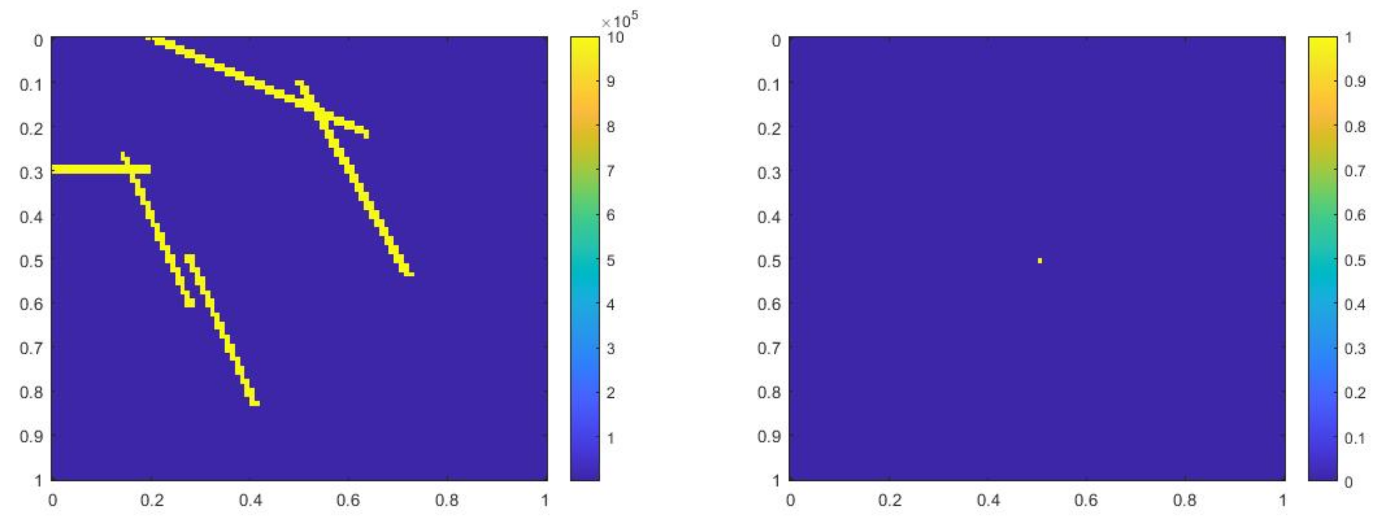
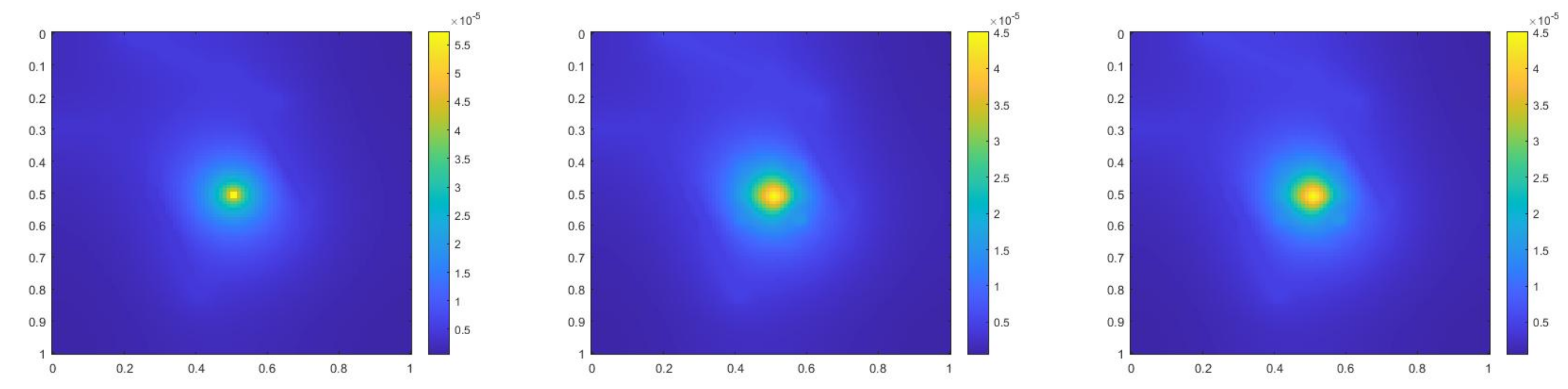
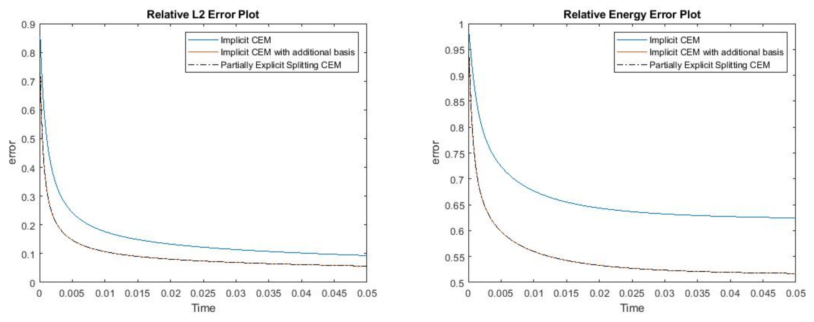
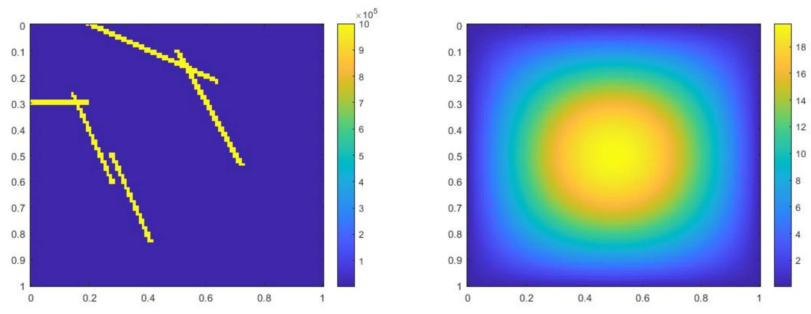
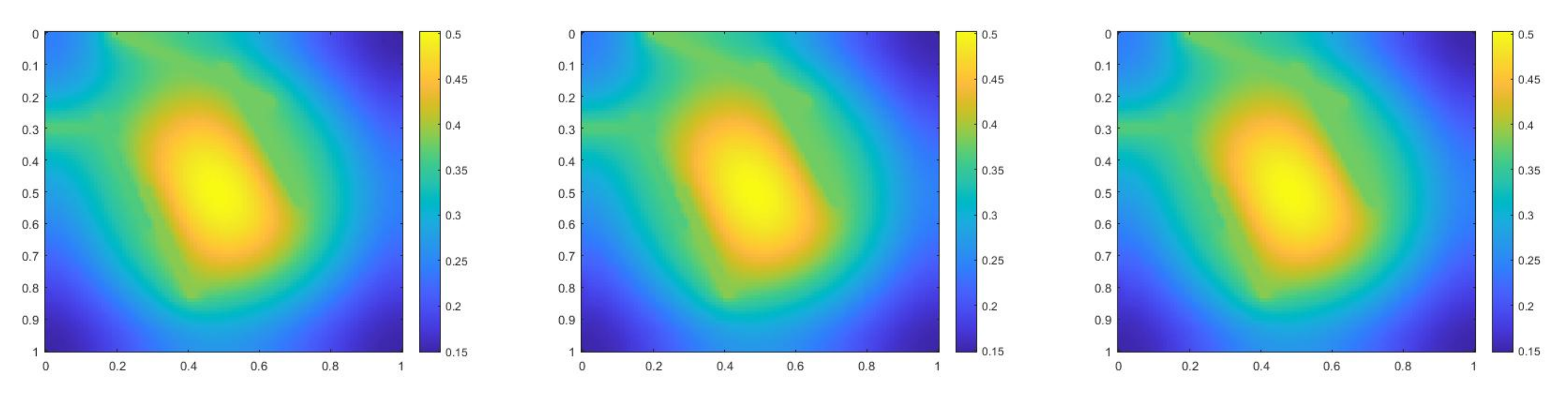
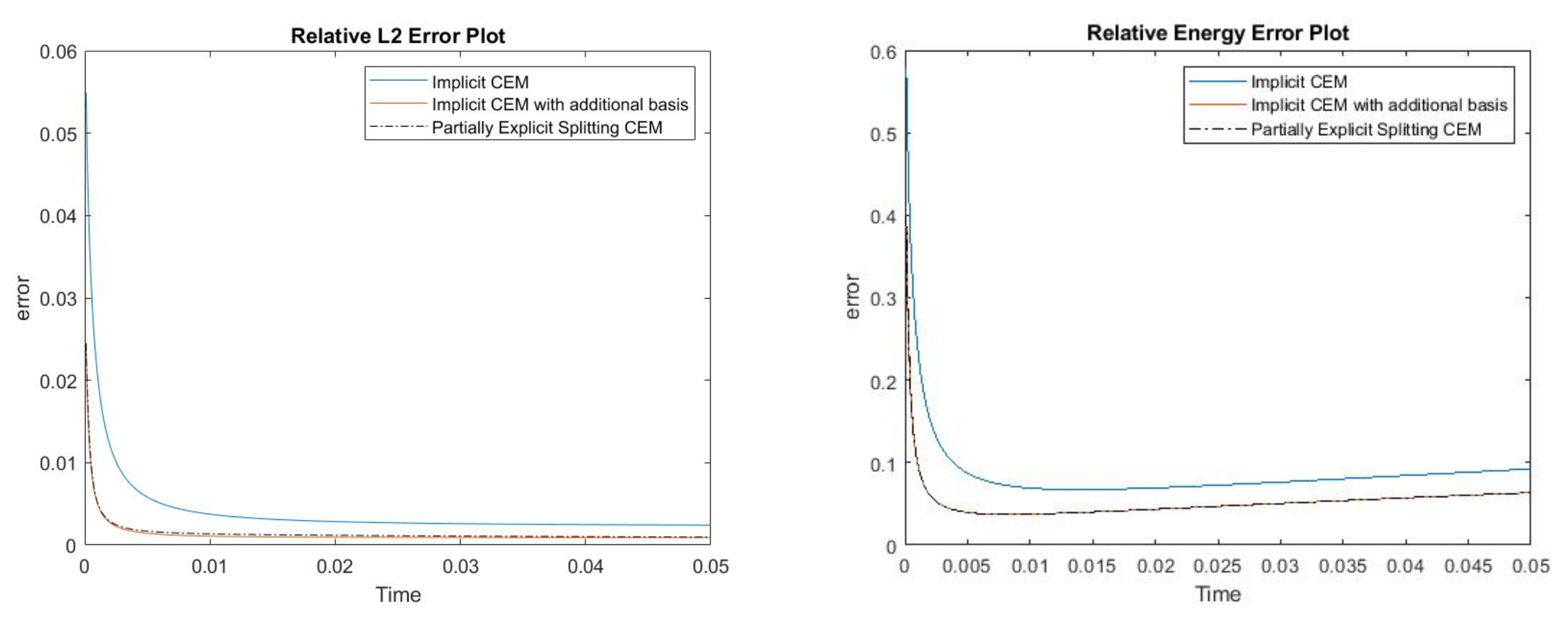
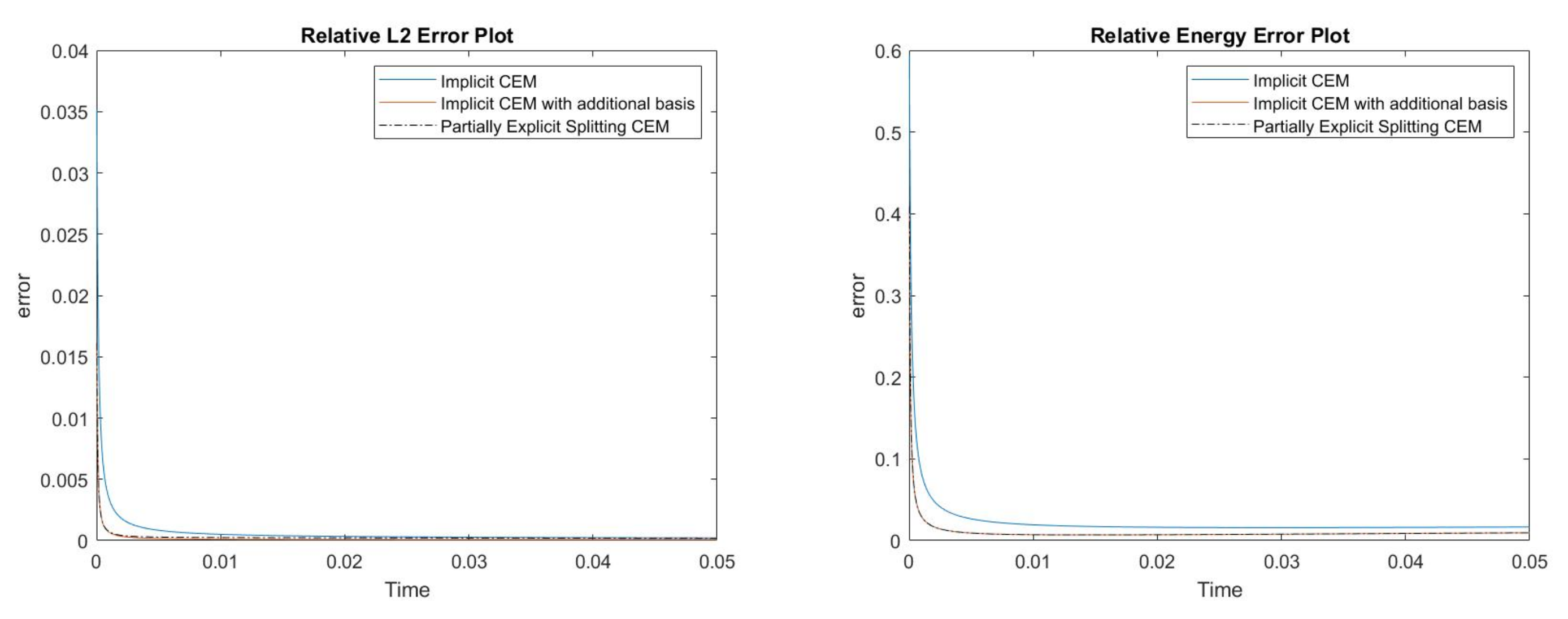
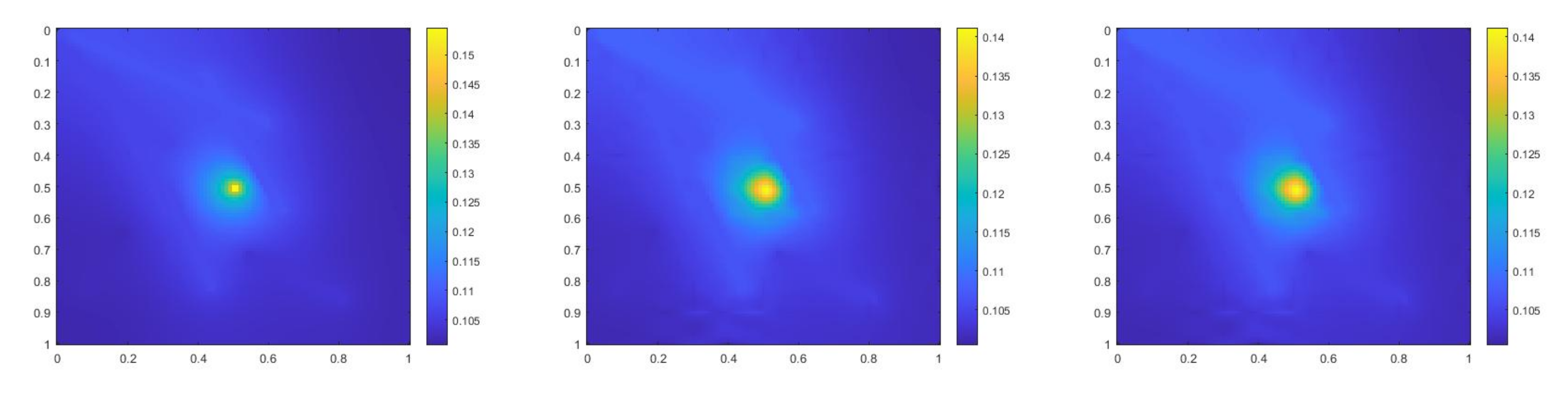
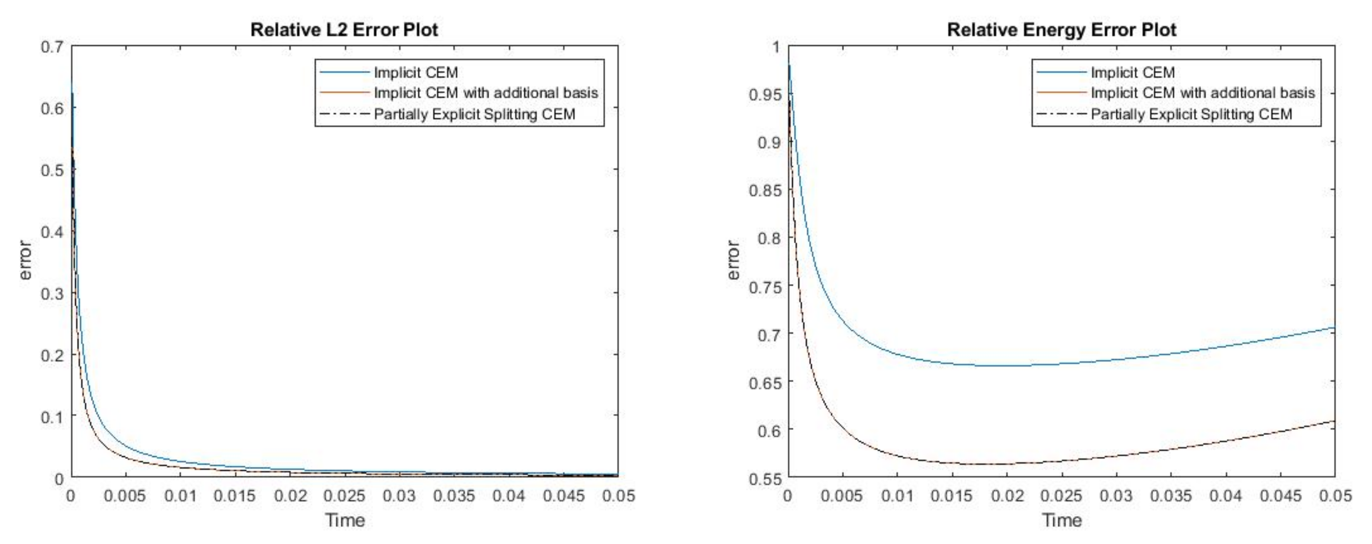
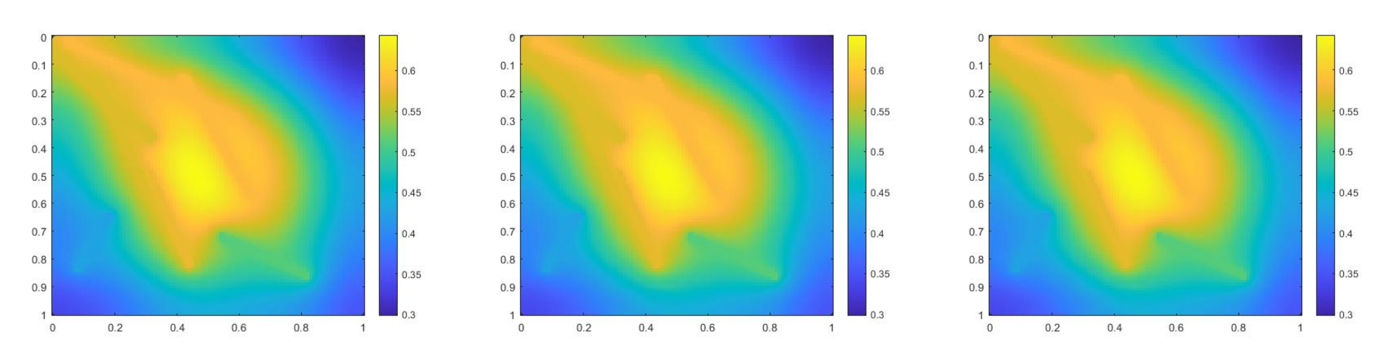
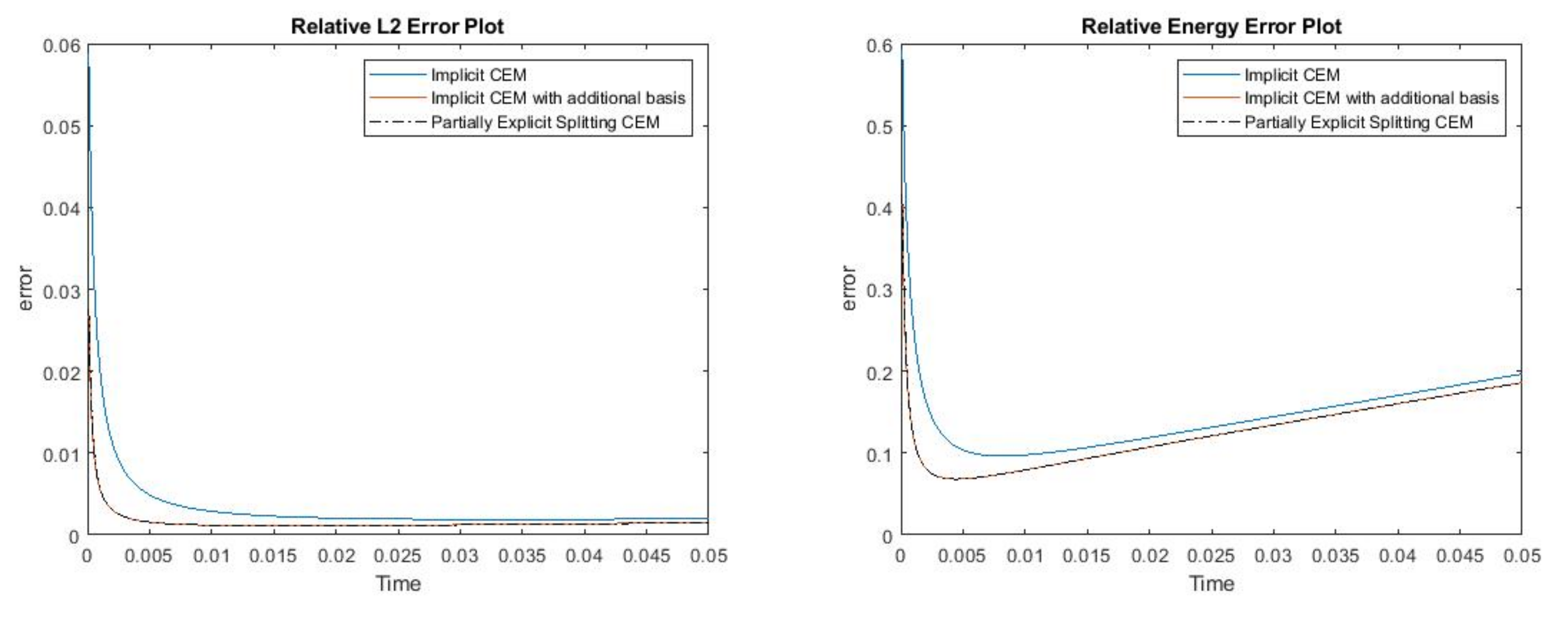
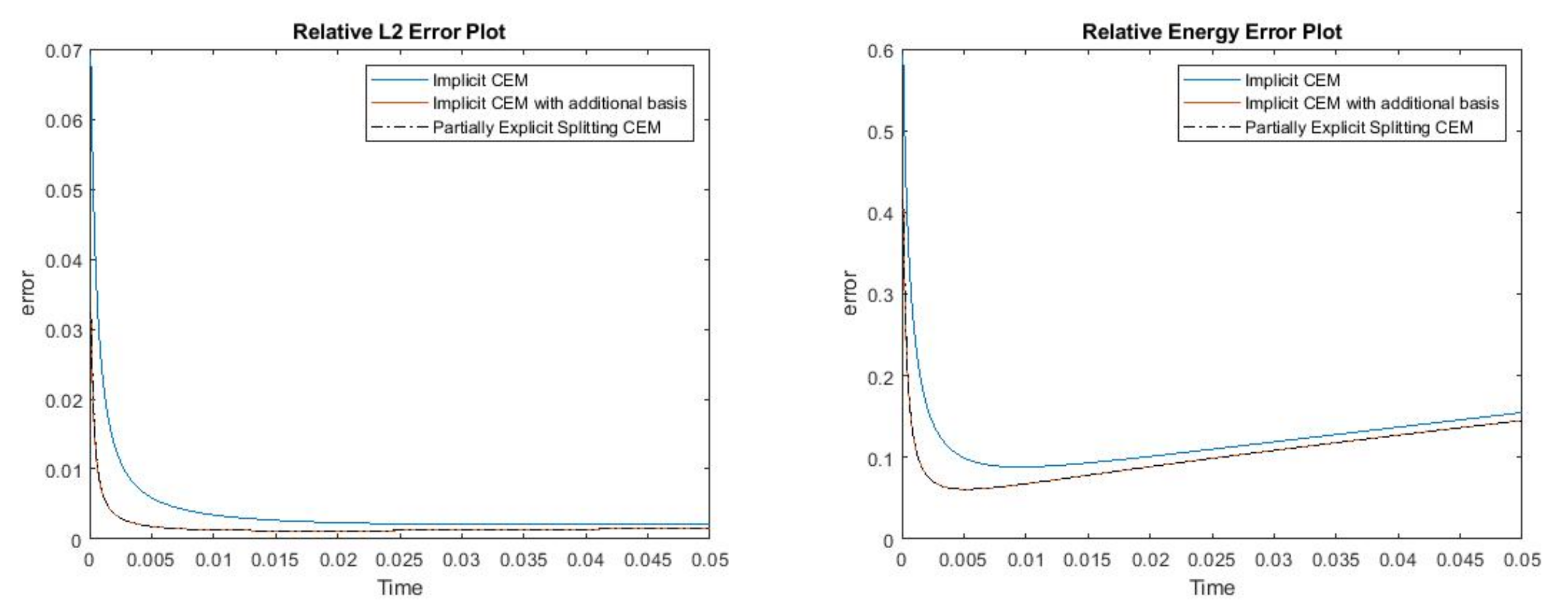
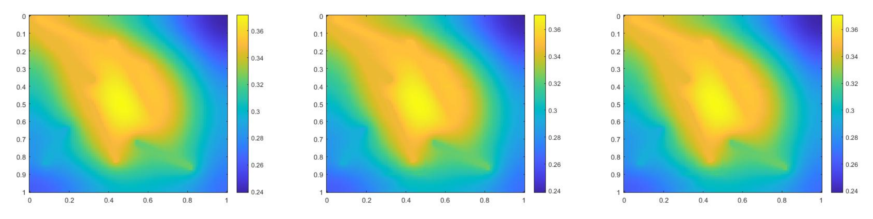
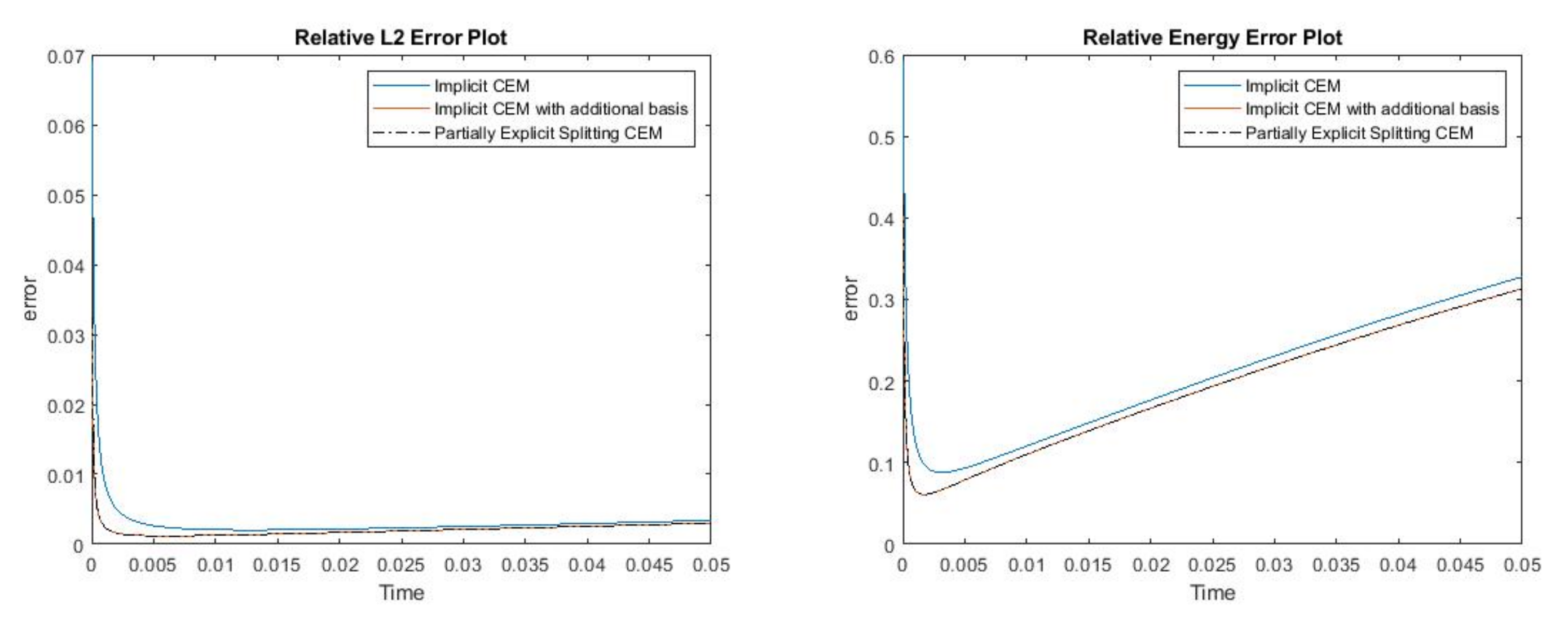
6. Numerical Results

In this section, we present numerical results for various cases. We consider several choices for f ( u ) and g ( u ) . For f ( u ) , we use diffusion operators for the linear case
f ( u ) = · ( κ u ) ,
and the nonlinear case
f ( u ) = · ( κ α ( u ) u ) .
In all examples, we use two heterogeneous high contrast κ ( x ) that represent the media, where one is more complex (more channels). We note that our approach can handle the general case κ = κ i j ( x , u ) . In the paper, we consider simpler cases to demonstrate our main concepts. As for g ( u ) , we consider several choices of nonlinear reaction terms, as discussed below. This term contains a nonlinear reaction and steady state spatial source term. One source term is more regular and the other more singular. The singular source term was chosen so that the CEM solution would require additional basis functions, as the source term contains subgrid features. In all numerical examples, the coarse mesh size was 1 10 and the fine mesh size was 1 100 . For the time discretization, we consider the final time T = 0.05 . In our numerical examples, we compare three methods.
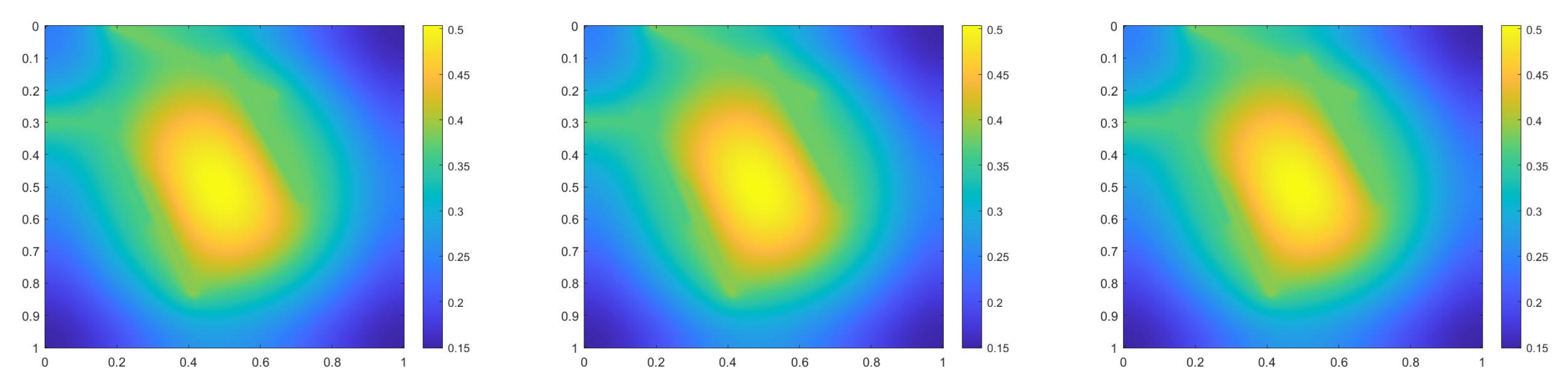
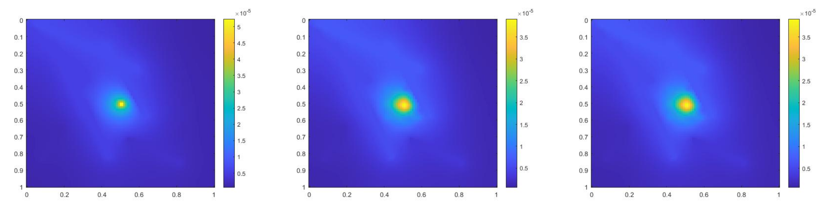
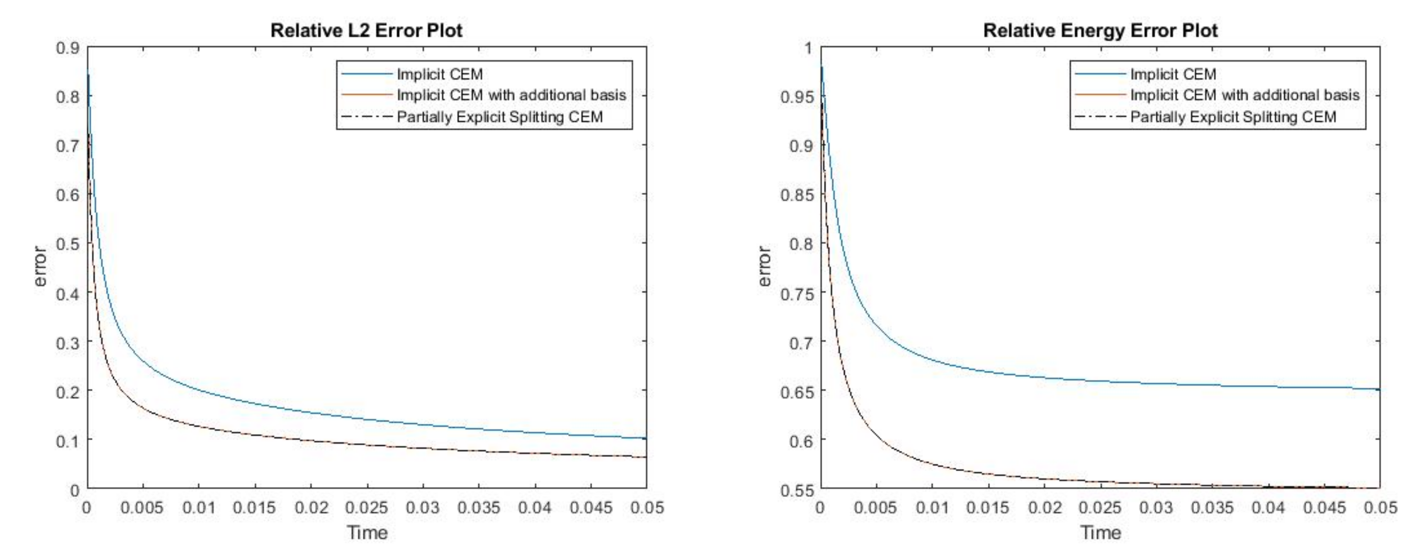
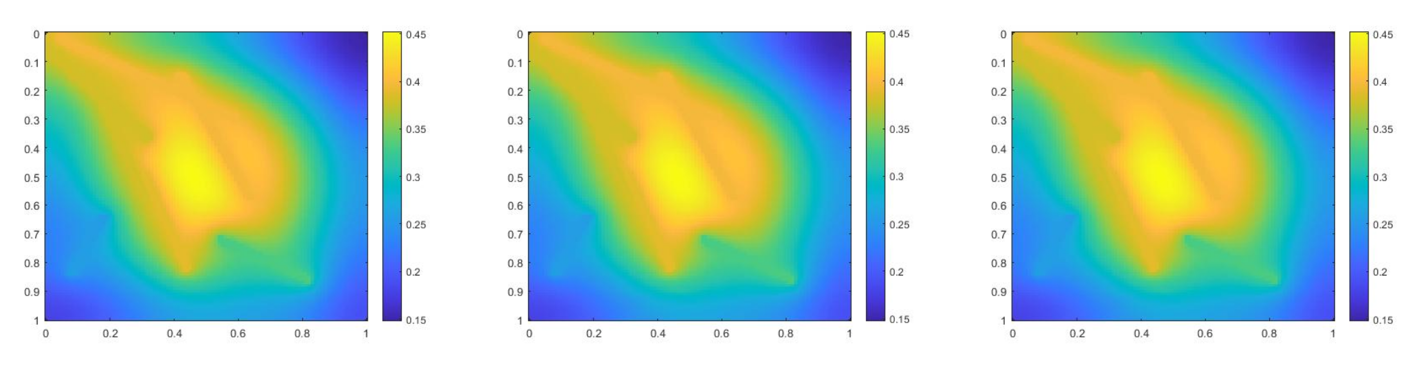
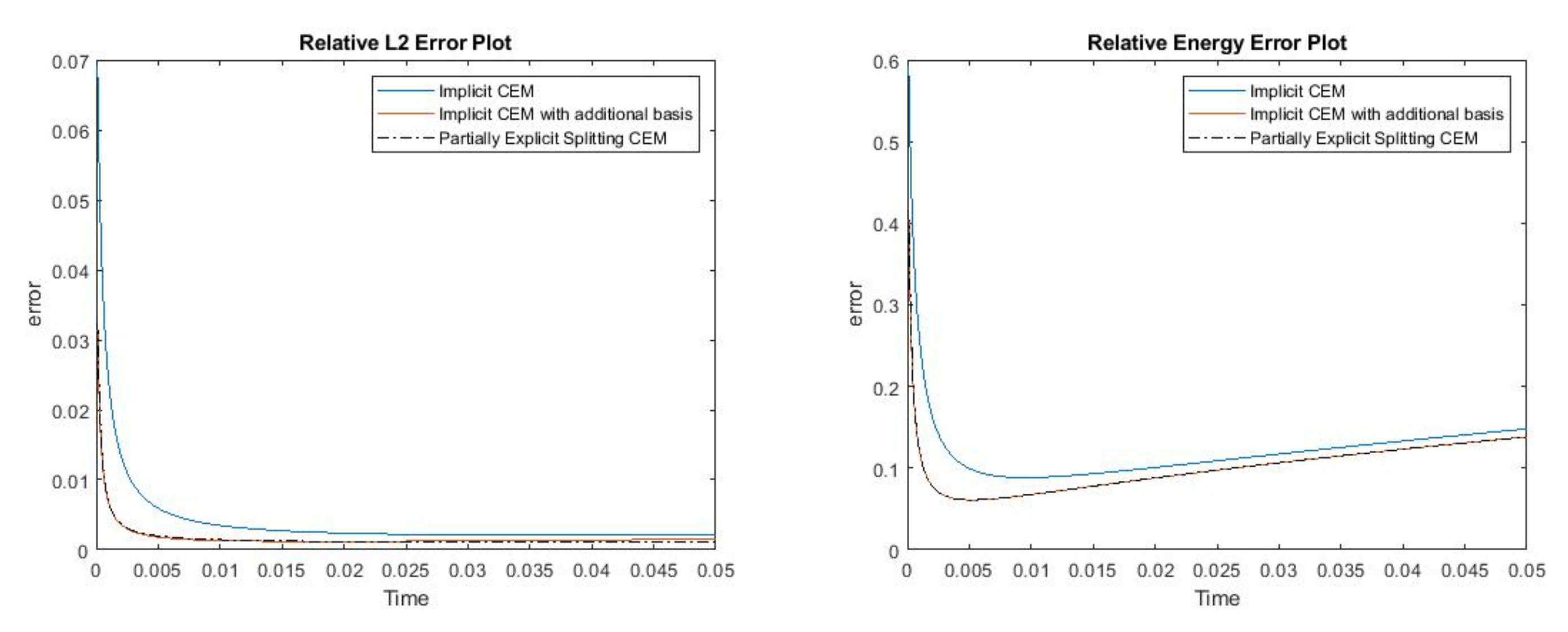
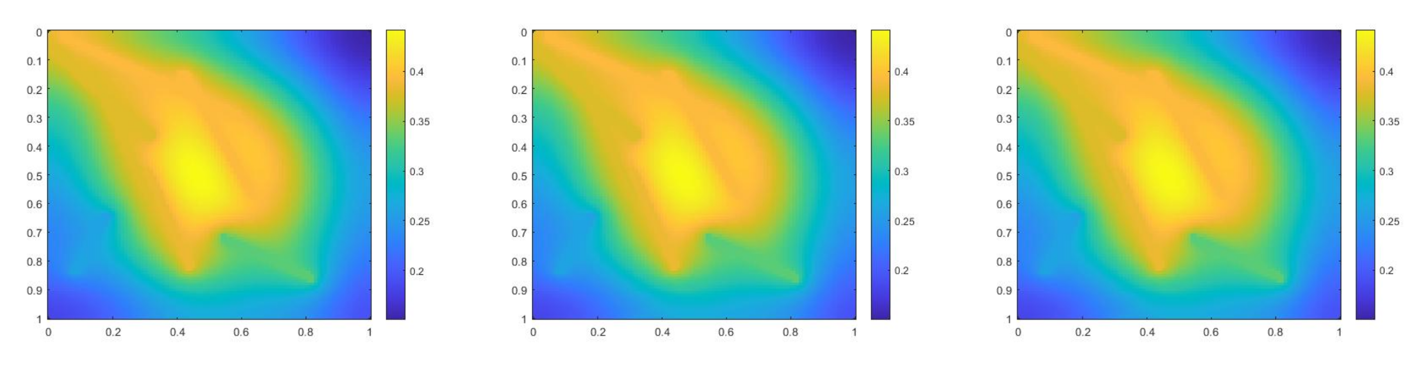
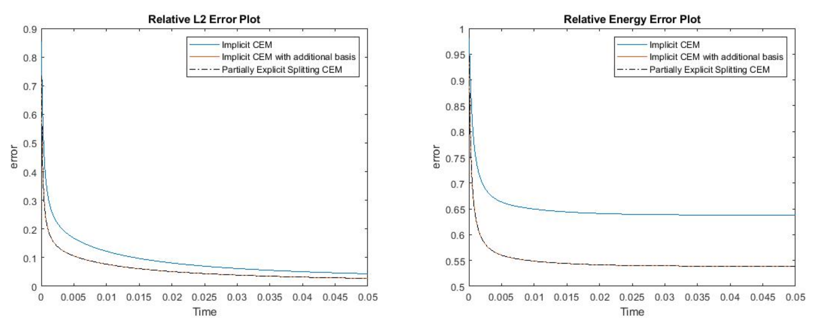
  • First, we used implicit CEM to compute the solution without additional degrees of freedom (called “Implicit CEM” in our graphs).
  • Secondly, we computed the solution with additional degrees of freedom using implicit CEM (called “Implicit CEM with additional basis” in our graphs).
  • Finally, we computed the solution with additional degrees of freedom using our proposed partially explicit approach (called “Partially Explicit Splitting CEM” in our graphs).
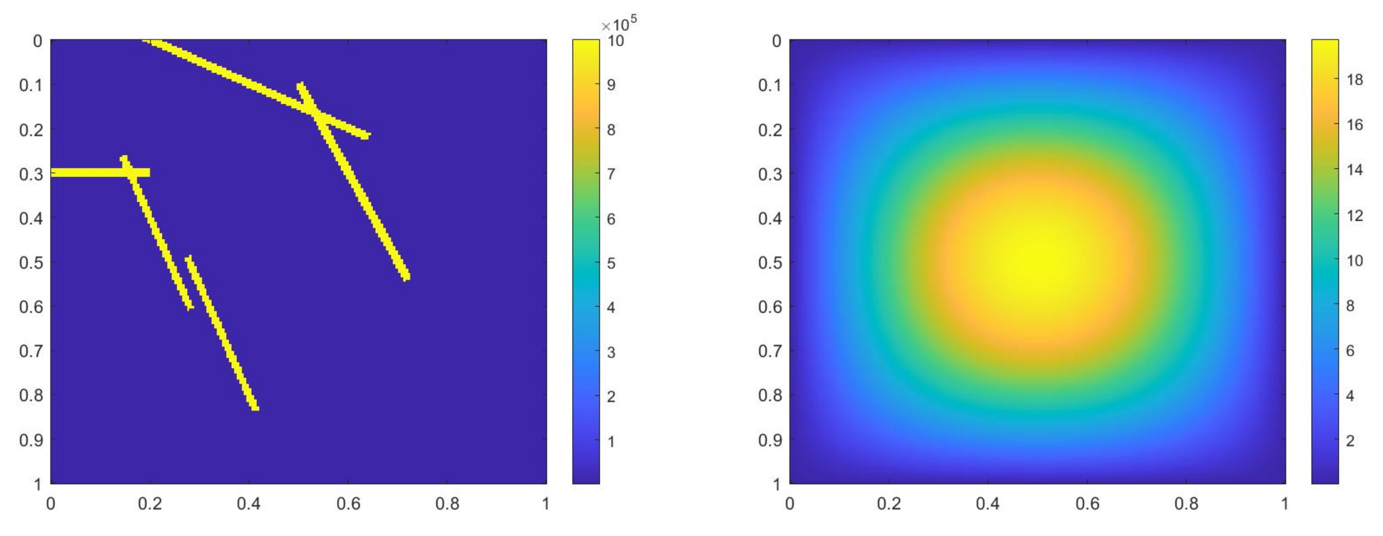
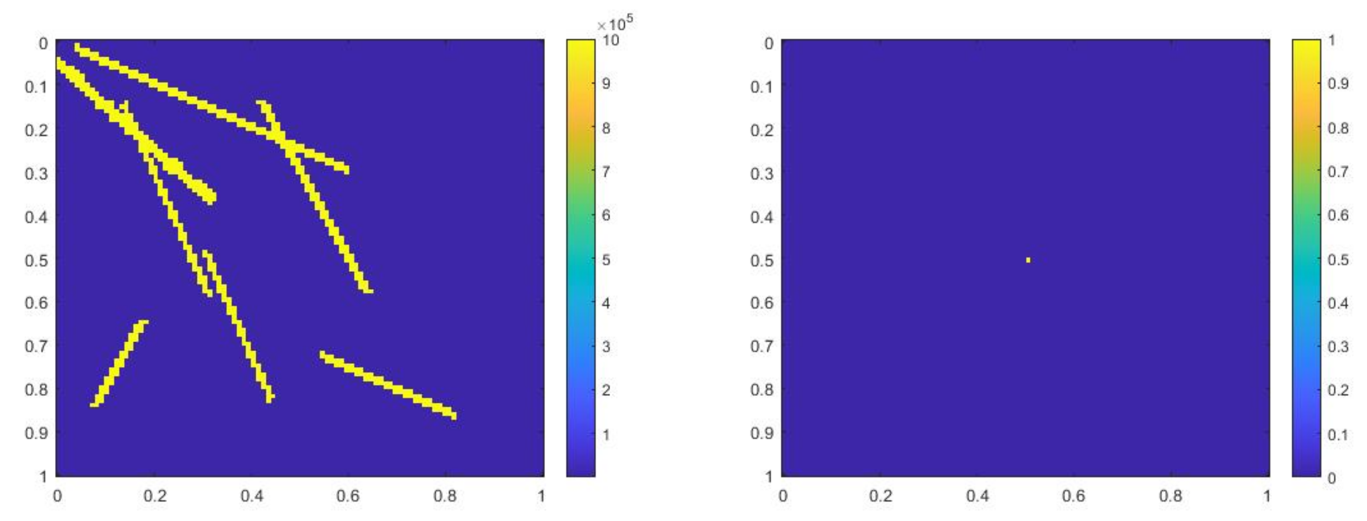
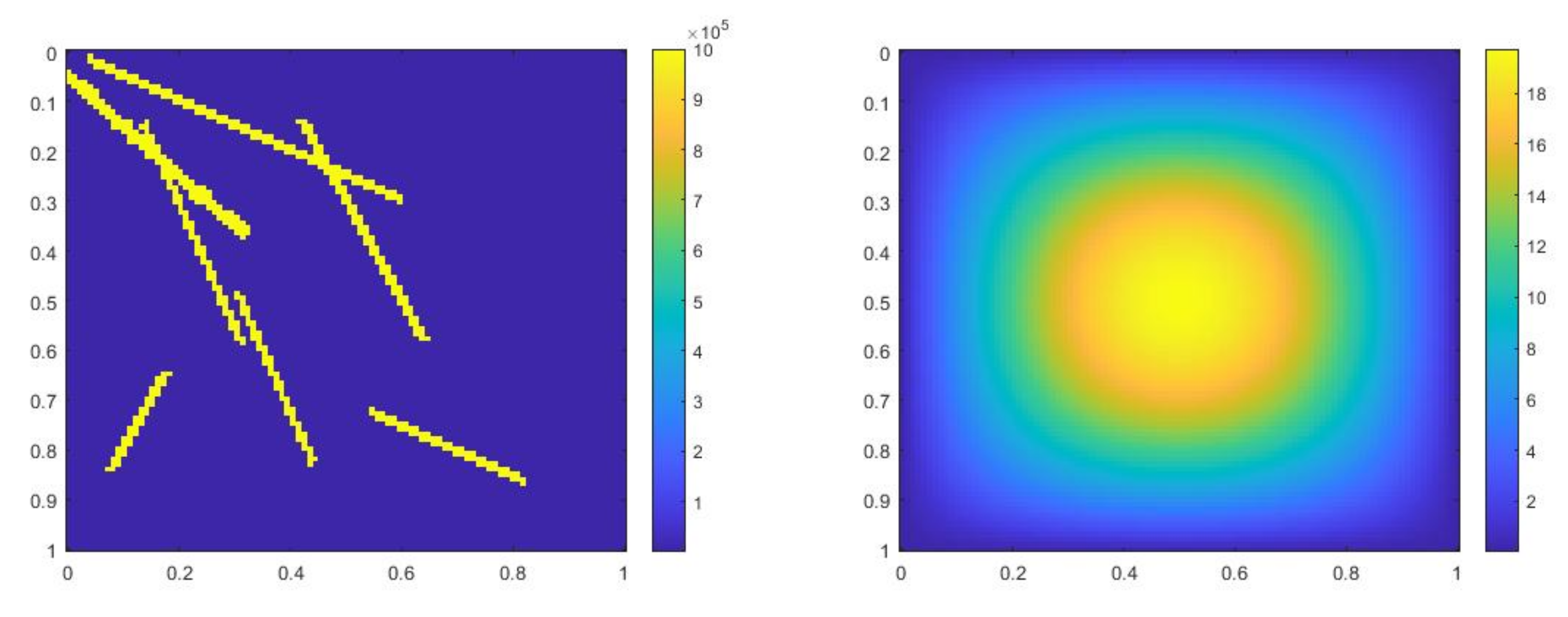
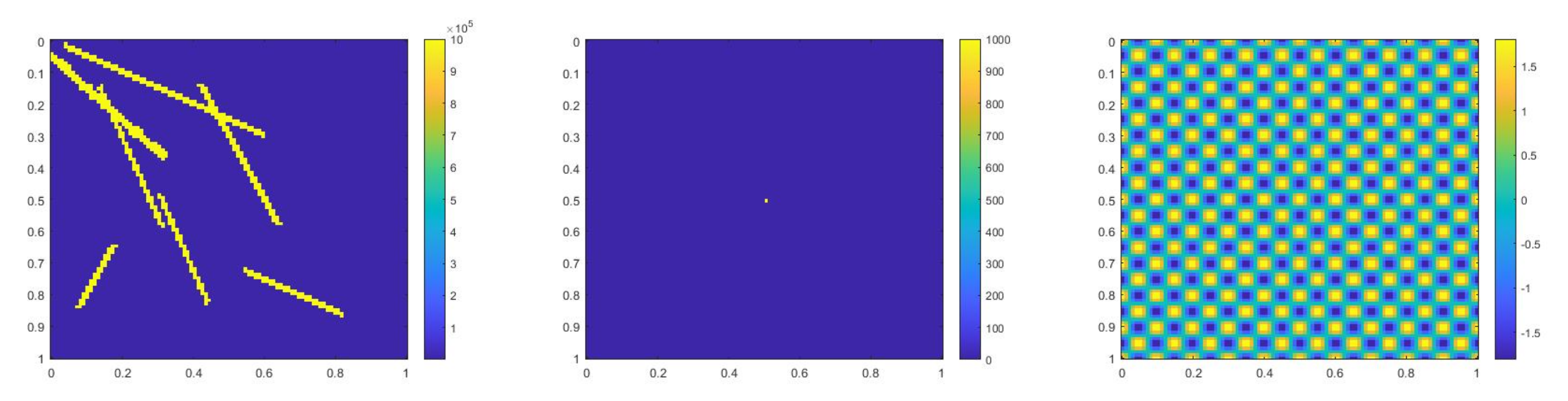
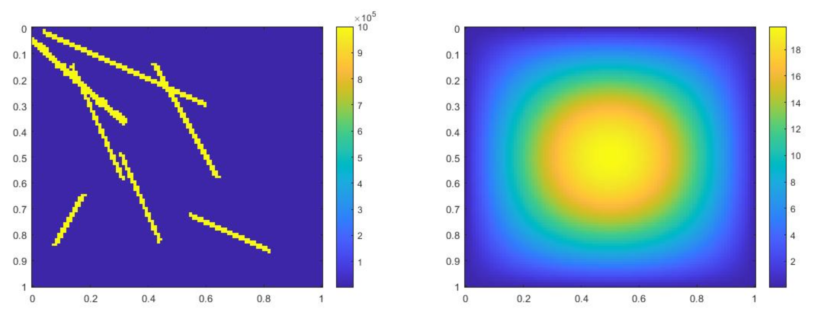
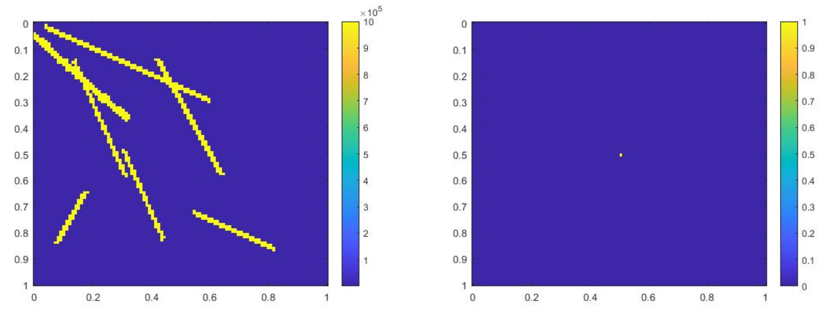
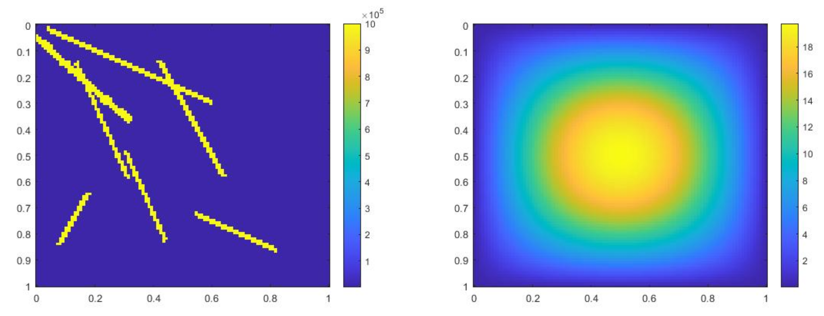
In all examples, we used Newton or Picard iterations to find the solutions of nonlinear equations. In all examples, our proposed partially explicit method provided similar accuracy as the implicit CEM approach that uses additional degrees of freedom.

6.1. V H , 1 and V H , 2 Constructions

In this section, we present a way to construct the spaces [3] satisfying (5).We used the CEM finite element space as V H , 1 . To find a V H , 2 satisfying the condition (5), we can use an eigenvalue problem to construct the local basis functions. We first introduce the CEM finite element space, followed by the discussion of constructing V H , 2 . In the following, we let V ( S ) = H 0 1 ( S ) for a proper subset S Ω .

6.1.1. CEM Method

In this section, we introduce the CEM method for solving the problem (2). We construct the finite element space by solving a constrained energy minimization problem. Let T H be a coarse grid partition of Ω . For K i T H , we first need to define a set of auxiliary basis functions in V ( K i ) . We solve
K i κ ψ j ( i ) · v s . = λ j ( i ) s i ( ψ j ( i ) , v ) v s . V ( K i ) ,
where
s i ( u , v ) = K i κ ˜ u v , κ ˜ = κ H 2 or κ ˜ = κ i χ i 2
with { χ i } being a partition of unity functions corresponding to an overlapping partition of the domain. We then collect the first L i eigenfunctions corresponding to the first L i smallest eigenvalues. We define
V a u x ( i ) : = span { ψ j ( i ) : 1 j L i } .
Next, we define a projection operator Π : L 2 ( Ω ) V a u x L 2 ( Ω )
s ( Π u , v ) = s ( u , v ) v V a u x : = i = 1 N e V a u x ( i ) ,
where s ( u , v ) : = i = 1 N e s i ( u | K i , v | K i ) and N e is the number of coarse elements. We let K i + be an oversampling domain of K i , which is a few coarse blocks larger than K i [11]. For each auxiliary basis functions ψ j ( i ) , we can find a local basis function ϕ j ( i ) V ( K i + ) such that
a ( ϕ j ( i ) , v ) + s ( μ j ( i ) , v ) = 0 v V ( K i + ) , s ( ϕ j ( i ) , ν ) = s ( ψ j ( i ) , ν ) ν V a u x ( K i + )
for some μ j ( i ) V a u x . We then define the space V c e m as
V c e m : = span { ϕ j ( i ) : 1 i N e , 1 j L i } .
The CEM solution u c e m is given by
( u c e m t , v ) + ( f ( u c e m ) + g ( u c e m ) , v s . ) = 0 v V c e m .
Let V ˜ : = { v V : Π ( v ) = 0 } , and we can now construct V H , 2 .

6.1.2. Construction of
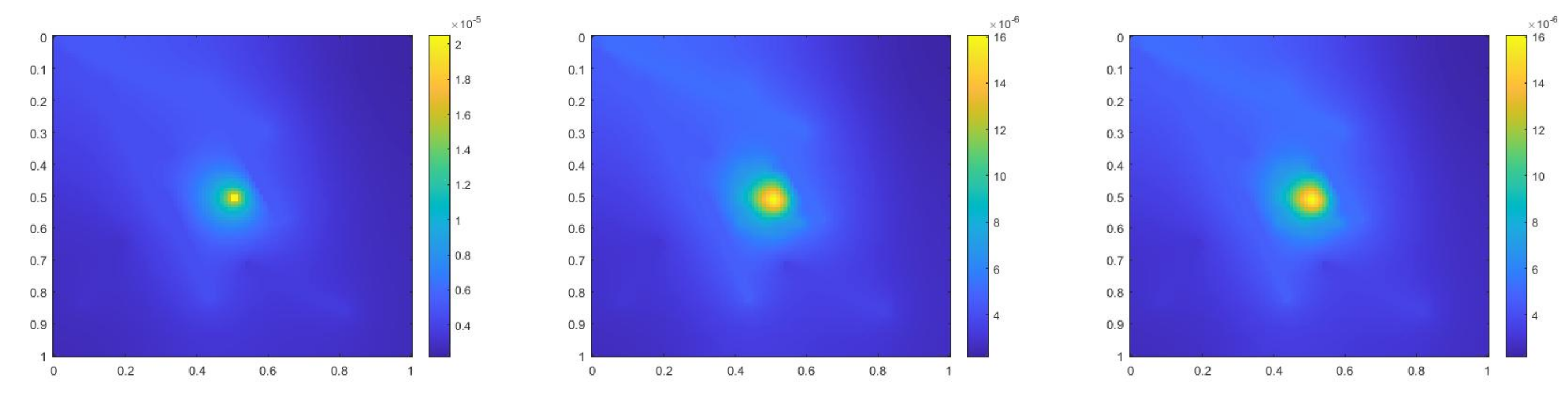
 V H , 2

The construction of V H , 2 is based on the CEM type finite element space. For each coarse element K i , we solve an eigenvalue problem to get the second type of auxiliary basis. We obtain eigenpairs ( ξ j ( i ) , γ j ( i ) ) ( V ( K i ) V ˜ ) × R by solving
K i κ ξ j ( i ) · v s . = γ j ( i ) K i ξ j ( i ) v , v V ( K i ) V ˜
and rearranging the eigenvalues by γ 1 ( i ) γ 2 ( i ) . For each K i , we choose the first few J i eigenfunctions corresponding to the smallest J i eigenvalues. We define V a u x , 2 : = span { ξ j ( i ) : 1 i N e , 1 j J i } . For each auxiliary basis function ξ j ( i ) V a u x , 2 , we define a basis function ζ j ( i ) V ( K i + ) such that μ j ( i ) , 1 V a u x , 1 , μ j ( i ) , 2 V a u x , 2 and
a ( ζ j ( i ) , v ) + s ( μ j ( i ) , 1 , v ) + ( μ j ( i ) , 2 , v ) = 0 , v V ( K i + ) ,
s ( ζ j ( i ) , ν ) = 0 , ν V a u x , 1 ,
( ζ j ( i ) , ν ) = ( ξ j ( i ) , ν ) , ν V a u x , 2 ,
where we use the notation V a u x , 1 to denote the space V a u x defined in Section 6.1.1. We define
V H , 2 = span { ζ j ( i ) | 1 i N e , 1 j J i } .

6.2. Linear F ( U )

In this subsection, we discuss the numerical results for
f ( u ) = · ( κ u ) .
Equation (1) becomes
u t · ( κ u ) + g ( u ) = 0 .
For the time discretization, we consider the time step Δ t = T 500 = 10 4 .
Let u h be the fine mesh solution for Equation (13). We use Newton’s method to solve the following implicit equation.
( u h n + 1 u h n Δ t , v ) + a ( u h n + 1 , v ) + ( g ( u h n + 1 ) , v ) = 0 v s . V h ,
where a ( u h n + 1 , v ) = Ω κ u h n + 1 · v s . and ( · , · ) is the L 2 inner product. In finite element methods, let { φ i } i be fine mesh basis functions. Let m be the step number in Newton’s method. We have u h n + 1 , m + 1 = i U h , i n + 1 , m + 1 φ i , u h n + 1 , m = i U h , i n + 1 , m φ i and u h n = i U h , i n φ i . Let M and A be the mass and stiffness matrices, respectively. Let U h n + 1 , m + 1 = ( U h , i n + 1 , m + 1 ) , U h n + 1 , m = ( U h , i n + 1 , m ) and U h n = ( U h , i n ) . We define
P ( U h n + 1 , m ) = M U h n + 1 , m + Δ t · A U h n + 1 , m + Δ t · G M U h n ,
where G = ( G i )
G i = ( g ( u h n + 1 , m ) , φ i ) .
Then,
( J P ) ( U h n + 1 , m ) = M + Δ t · A + Δ t · ( J G ) ,
where J G = ( ( J G ) i j )
( J G ) i j = ( g ( u h n + 1 , m ) , φ i ) U h , j n + 1 , m .
Then, we have
U h n + 1 , m + 1 = U h n + 1 , m ( J P ) 1 ( U h n + 1 , m ) P ( U h n + 1 , m ) .
Newton’s method for the coarse mesh is similar and we do not show the details. The partially explicit scheme is:
( u H , 1 n + 1 u H , 1 n Δ t + u H , 2 n u H , 2 n 1 Δ t , v 1 ) + a ( ( u H , 1 n + 1 + u H , 2 n ) , v 1 ) + ( g ( u H , 1 n + u H , 2 n ) , v 1 ) = 0 v 1 V H , 1 , ( u H , 2 n + 1 u H , 2 n Δ t + u H , 1 n u H , 1 n 1 Δ t , v 2 ) + a ( ( u H , 1 n + 1 + u H , 2 n ) , v 2 ) + ( g ( u H , 1 n + u H , 2 n ) , v 2 ) = 0 v 2 V H , 2 .
In our first example, we consider
g ( u ) = ( 10 · u · ( u 2 1 ) + g 0 ) ,
where g 0 = g δ ( x ) , g δ ( x ) is 1 at the fine-grid element containing ( 1 / 2 , 1 / 2 ) and 0 otherwise. In Figure 1, the permeability field ( κ ) and g 0 are presented. As is shown, this permeability field has heterogeneous high contrast channels, and g 0 is a singular source term. In Figure 2, we first present the reference solution which is implicitly solved using fine grid basis functions. The middle plot in Figure 2 is an implicit CEM solution obtained with additional basis functions, and the solution in the right plot is obtained using the partially explicit scheme presented above. These three plots all show the solution at t = T . We present two relative error plots in Figure 3. The first one is the relative L 2 error plot and the second one is the relative energy error plot. The blue, red and black curves (in both plots) stand for the relative errors for the implicit CEM solution, the implicit CEM solution (with additional basis) and the partially explicit solution, respectively. In each of these two plots, there is a noticeable improvement for error when we use additional basis functions. We find that the black curve coincides with the red curve, which means that the partially explicit scheme can achieve similar accuracy as the fully implicit scheme.
In this case,
g ( u ) = ( 10 · u · ( u 2 1 ) + g 0 ) ,
where g 0 = 2 π 2 sin ( π x ) sin ( π y ) . The difference is that we use a smooth source term. In Figure 4, the permeability field κ and source term g 0 are shown. The reference solution at the final time, implicit CEM solution (with additional basis) at the final time and partially explicit solution at the final time are presented in Figure 5. We show the relative L 2 error plot and the relative energy error plot in Figure 6. We see that the relative L 2 and energy error curves for implicit CEM (with additional basis) and partially explicit scheme almost coincide, which implies similar accuracy between them.
In the next example, we test our proposed method on the coarse mesh 1 20 and the fine mesh size 1 200 . We decrease the coarse mesh size of our previous example. The reaction term is
g ( u ) = ( 10 · u · ( u 2 1 ) + g 0 ) ,
where g 0 = 2 π 2 sin ( π x ) sin ( π y ) . The permeability field and the source term g 0 are shown in Figure 7. The reference solution, the implicit CEM solution (with additional basis) and the partially explicit solution are presented in Figure 8. We show the relative L 2 error plot and the relative energy error plot in Figure 9. From these two error plots, we see that the proposed partially explicit scheme can achieve accuracy similar to the implicit CEM scheme (with additional basis). If we compare these results to our previous example (see Figure 6), we can observe that the errors are smaller when using finer coarse mesh sizes. In particular, we observe a four-fold error reduction in L 2 norm and a six-fold error reduction in the energy norm at t 0.05 . Moreover, we observe that the energy error does not have a slight increase if we use a smaller coarse mesh size.
In the next numerical example,
g ( u ) = ( 10 · u · ( u 2 1 ) + g 0 ) ,
where g 0 = g δ ( x ) , g δ ( x ) is 1 at the fine-grid element containing ( 1 / 2 , 1 / 2 ) and 0 otherwise. We use a more complicated permeability field with more high contrast channels. Figure 10 shows the permeability field κ and source term g 0 . The reference solution at t = T , implicit CEM solution (with additional basis) at t = T and partially explicit solution at t = T are presented in Figure 11. In Figure 12, we show the relative L 2 error plot and the relative energy error plot. In this case, in both error plots, the curves for implicit CEM (with additional basis) and partially explicit scheme coincide. We note that the energy error is large in this case, as we choose the case where there are not sufficient multiscale degrees of freedom added. Consequently, there is room for improvement. Our objective is to show that our proposed approach performs similarly to a fully implicit approach. Moreover, the L 2 error is small and the solution profile looks similar to the fine grid solution.
In this example,
g ( u ) = ( 10 · u · ( u 2 1 ) + g 0 ) ,
where g 0 = 2 π 2 sin ( π x ) sin ( π y ) . We use the more complicated permeability field and the smooth source term, which are shown in Figure 13. In Figure 14, the reference solution at the final time, implicit CEM solution (with additional basis) at the final time and partially explicit solution at the final time are presented. Relative L 2 error and energy error plots are shown in Figure 15. In this case, the relative error for the implicit CEM scheme is small and comparable to the two schemes with additional basis functions. From Figure 15, we can see that the L 2 and energy error for implicit CEM (with additional basis) and the partially explicit scheme are nearly the same. We note that the relative energy error of our scheme is slightly higher; however, the proposed approach is stable, as it performs similarly to the fully implicit method.
In this case, we use a new reaction term
g = ( 1 + cos ( a 1 · u ) + g 0 ) , a 1 ( x , y ) = 2 cos ( 20 π x ) cos ( 20 π y )
and g 0 = g δ ( x ) , g δ ( x ) is 1 at the fine-grid element containing ( 1 / 2 , 1 / 2 ) and 0 otherwise. In numerical experiments, we set a 1 to be constant inside every fine element. Figure 16 shows the permeability field κ , the source term g 0 and the function a 1 . The reference solution, implicit CEM solution (with additional basis) and partially explicit solution at the final time are shown in Figure 17. The relative L 2 error plot and relative energy error plot are presented in Figure 18. From the relative L 2 error plot, we can see that the relative L 2 errors for the three schemes are comparable. For the relative energy error, we find a large improvement when we introduce an additional basis function. The relative energy errors for the implicit CEM solution (with additional basis) and partially explicit solution are nearly the same.
In this case, we take
g = ( 1 + cos ( a 1 · u ) + g 0 ) , a 1 ( x , y ) = 2 cos ( 20 π x ) cos ( 20 π y )
and g 0 = 2 π 2 sin ( π x ) sin ( π y ) . The permeability field κ , the source term g 0 and the function a 1 are presented in Figure 19. The reference solution, implicit CEM solution (with additional basis) and partially explicit solution at the final time are shown in Figure 20. We present the relative L 2 error plot and the relative energy error plot in Figure 21. We can observe that the L 2 and energy error curves for implicit CEM (with additional basis) and partially explicit scheme coincide.

6.3. Nonlinear F ( U )

We would like to explore the case in which the diffusion operator is nonlinear. This, in Equation (1), we set
f ( u ) = · ( κ α ( u ) u ) .
Equation (1) becomes
u t · ( κ α ( u ) u ) + g ( u ) = 0 .
Let u h be the fine mesh solution for Equation (14). We use the Picard–Newton iteration to solve the implicit equation.
u h n + 1 , m + 1 u h n Δ t , v + Ω κ α ( u h n + 1 , m ) u h n + 1 , m + 1 · v s . + ( g ( u h n + 1 , m + 1 ) , v ) = 0 v V h ,
where m is the Picard–Newton step number and ( · , · ) is the L 2 inner product. In finite element methods, let { φ i } i be fine mesh basis functions. We have u h n + 1 , m + 1 = i U h , i n + 1 , m + 1 φ i , u h n + 1 , m = i U h , i n + 1 , m φ i and u h n = i U h , i n φ i . Let M be the mass matrix. Let U h n + 1 , m + 1 = ( U h , i n + 1 , m + 1 ) , U h n + 1 , m = ( U h , i n + 1 , m ) and U h n = ( U h , i n ) . We define
Q ( U h n + 1 , m ) = M U h n + 1 , m + Δ t · A U h n + 1 , m M U h n + Δ t · G ,
where A = ( A i j )
A i j = Ω κ α ( u h n + 1 , m ) φ j φ i
and G = ( G i )
G i = ( g ( u h n + 1 , m ) , φ i ) .
Then,
( J Q ) ( U h n + 1 , m ) = M + Δ t A + Δ t · ( J G ) ,
where J G = ( ( J G ) i j )
( J G ) i j = ( g ( u h n + 1 , m ) , φ i ) U h , j n + 1 , m .
Thus,
U h n + 1 , m + 1 = U h n + 1 , m ( J Q ) 1 ( U h n + 1 , m ) Q ( U h n + 1 , m ) .
Newton’s method for a coarse mesh is similar. For the partially explicit scheme, we use the following Picard–Newton iteration which can be solved similarly using the method introduced above. Note that we change the reaction term to be partially explicit.
( u H , 1 n + 1 , m + 1 u H , 1 n Δ t + u H , 2 n u H , 2 n 1 Δ t , v 1 ) + Ω κ α ( u H , 1 n + 1 , m + u H , 2 n ) ( u H , 1 n + 1 , m + 1 + u H , 2 n ) · v 1 = ( g ( u H , 1 n + 1 , m + 1 + u H , 2 n ) , v 1 ) v 1 V H , 1 , ( u H , 2 n + 1 u H , 2 n Δ t + u H , 1 n u H , 1 n 1 Δ t , v 2 ) + Ω κ α ( u H , 1 n + 1 + u H , 2 n ) ( u H , 1 n + 1 + u H , 2 n ) · v 2 = ( g ( u H , 1 n + 1 + u H , 2 n ) , v 2 ) v 2 V H , 2 .
In the following three examples, we use g ( u H , 1 n + 1 + u H , 2 n ) in the partially explicit algorithm. One can prove its stability as in Lemma 1 and Lemma 2. The proof is similar, and we omit it here.
In the following three cases,
g ( u ) = ( 10 u ( u 2 1 ) + g 0 ) .
In the first example, we consider α ( u ) = 1 + u 2 , g 0 = 2 π 2 sin ( π x ) sin ( π y ) and the time step Δ t = T 500 = 10 4 . The permeability field κ and the source term g 0 are presented in Figure 22. The reference solution, implicit CEM solution (with additional basis) and partially explicit solution at the final time are shown in Figure 23. We present the relative L 2 error plot and relative energy error plot in Figure 24. We observe that the curves for implicit CEM solution (with additional basis) and partially explicit solution coincide, which implies that our new partially explicit scheme is also effective and has similar accuracy to the implicit CEM (with additional basis) scheme.
In the second example, we consider α ( u ) = 2 + cos ( u ) , g 0 = g δ ( x ) , and g δ ( x ) is 1 at the fine-grid element containing ( 1 / 2 , 1 / 2 ) and 0 otherwise. Figure 25 shows the permeability field κ and the source term g 0 . The reference solution, implicit CEM solution (with additional basis) and partially explicit solution at t = T are presented in Figure 26. The relative L 2 error plot and relative energy error plot are shown in Figure 27. The partially explicit scheme also works in this case, and gives similar accuracy as the implicit CEM (with additional basis) scheme.
In this case, we use α ( u ) = 2 + cos ( u ) , g 0 = 2 π 2 sin ( π x ) sin ( π y ) and the time step Δ t = 0.05 1500 . The permeability field κ and the source term g 0 are presented in Figure 28. We show the reference solution, implicit CEM solution (with additional basis) and partially explicit solution at t = T in Figure 29. The relative L 2 error plot and the relative energy error plot are presented in Figure 30. From Figure 30, we see that the curves for implicit CEM (with additional basis) and partially explicit scheme coincide, which implies that they have similar accuracy.

7. Conclusions

In this work, we design and analyze contrast-independent time discretization for nonlinear problems. The work continues our earlier work on linear problems, where we proposed temporal splitting and associated spatial decomposition that guarantees stability. We introduce two spatial spaces, the first accounting for spatial features related to fast time scales and the second for spatial features related to “slow” time scales. We propose time splitting, wherein the first equation solves for fast components implicitly and the second equation solves for slow components explicitly. We introduce a condition for multiscale spaces that guarantees the stability of the proposed splitting algorithm. Our proposed method is still implicit via mass matrix; however, it is explicit in terms of stiffness matrix for the slow component. We present numerical results, which show that the proposed methods provide very similar results to fully implicit methods.

Author Contributions

All authors (E.T.C., Y.E., W.T.L., W.L.) contributed to conceptualization, methodology, and writing the manuscript. All authors have read and agreed to the published version of the manuscript.

Funding

This research received no external funding.

Acknowledgments

The research of Eric Chung is partially supported by the Hong Kong RGC General Research Fund (project numbers 14304719 and 14302018), and the CUHK Faculty of Science, Direct Grant 2020-21. YE would like to thank the partial support from NSF 1620318 and 1934904. YE would also like to acknowledge the support of Mega-grant of the Russian Federation Government (N 14.Y26.31.0013).

Conflicts of Interest

The authors declare no conflict of interest.

References

  1. Ehlers, W. Darcy, Forchheimer, Brinkman and Richards: Classical hydromechanical equations and their significance in the light of the TPM. Arch. Appl. Mech. 2020, 1–21. [Google Scholar] [CrossRef]
  2. Bear, J. Dynamics of Fluids in Porous Media; Courier Corporation: North Chelmsford, MA, USA, 2013. [Google Scholar]
  3. Chung, E.T.; Efendiev, Y.; Leung, W.T.; Vabishchevich, P.N. Contrast-independent partially explicit time discretizations for multiscale flow problems. arXiv 2021, arXiv:2101.04863. [Google Scholar] [CrossRef]
  4. Chung, E.T.; Efendiev, Y.; Leung, W.T.; Vabishchevich, P.N. Contrast-independent partially explicit time discretizations for multiscale wave problems. arXiv 2021, arXiv:2102.13198. [Google Scholar]
  5. Efendiev, Y.; Hou, T. Multiscale Finite Element Methods: Theory and Applications; Surveys and Tutorials in the Applied Mathematical Sciences; Springer: New York, NY, USA, 2009; Volume 4. [Google Scholar]
  6. Le Bris, C.; Legoll, F.; Lozinski, A. An MsFEM type approach for perforated domains. Multiscale Model. Simul. 2014, 12, 1046–1077. [Google Scholar] [CrossRef] [Green Version]
  7. Hou, T.; Wu, X. A multiscale finite element method for elliptic problems in composite materials and porous media. J. Comput. Phys. 1997, 134, 169–189. [Google Scholar] [CrossRef] [Green Version]
  8. Jenny, P.; Lee, S.; Tchelepi, H. Multi-scale finite volume method for elliptic problems in subsurface flow simulation. J. Comput. Phys. 2003, 187, 47–67. [Google Scholar] [CrossRef]
  9. Chung, E.T.; Efendiev, Y.; Hou, T. Adaptive multiscale model reduction with generalized multiscale finite element methods. J. Comput. Phys. 2016, 320, 69–95. [Google Scholar] [CrossRef] [Green Version]
  10. Efendiev, Y.; Galvis, J.; Hou, T. Generalized multiscale finite element methods (GMsFEM). J. Comput. Phys. 2013, 251, 116–135. [Google Scholar] [CrossRef] [Green Version]
  11. Chung, E.T.; Efendiev, Y.; Leung, W.T. Constraint energy minimizing generalized multiscale finite element method. Comput. Methods Appl. Mech. Eng. 2018, 339, 298–319. [Google Scholar] [CrossRef] [Green Version]
  12. Chung, E.T.; Efendiev, Y.; Leung, W.T. Constraint energy minimizing generalized multiscale finite element method in the mixed formulation. Comput. Geosci. 2018, 22, 677–693. [Google Scholar] [CrossRef] [Green Version]
  13. Chung, E.T.; Efendiev, Y.; Leung, W.T.; Vasilyeva, M.; Wang, Y. Non-local multi-continua upscaling for flows in heterogeneous fractured media. J. Comput. Phys. 2018, 372, 22–34. [Google Scholar] [CrossRef] [Green Version]
  14. Owhadi, H.; Zhang, L. Metric-based upscaling. Comm. Pure. Appl. Math. 2007, 60, 675–723. [Google Scholar] [CrossRef]
  15. E, W.; Engquist, B. Heterogeneous multiscale methods. Comm. Math. Sci. 2003, 1, 87–132. [Google Scholar] [CrossRef] [Green Version]
  16. Henning, P.; Målqvist, A.; Peterseim, D. A localized orthogonal decomposition method for semi-linear elliptic problems. ESAIM Math. Model. Numer. Anal. 2014, 48, 1331–1349. [Google Scholar] [CrossRef] [Green Version]
  17. Roberts, A.; Kevrekidis, I. General tooth boundary conditions for equation free modeling. SIAM J. Sci. Comput. 2007, 29, 1495–1510. [Google Scholar] [CrossRef]
  18. Samaey, G.; Kevrekidis, I.; Roose, D. Patch dynamics with buffers for homogenization problems. J. Comput. Phys. 2006, 213, 264–287. [Google Scholar] [CrossRef] [Green Version]
  19. Hou, T.Y.; Li, Q.; Zhang, P. Exploring the locally low dimensional structure in solving random elliptic PDEs. Multiscale Model. Simul. 2017, 15, 661–695. [Google Scholar] [CrossRef] [Green Version]
  20. Hou, T.Y.; Ma, D.; Zhang, Z. A model reduction method for multiscale elliptic PDEs with random coefficients using an optimization approach. Multiscale Model. Simul. 2019, 17, 826–853. [Google Scholar] [CrossRef] [Green Version]
  21. Hou, T.Y.; Huang, D.; Lam, K.C.; Zhang, P. An adaptive fast solver for a general class of positive definite matrices via energy decomposition. Multiscale Model. Simul. 2018, 16, 615–678. [Google Scholar] [CrossRef] [Green Version]
  22. Brown, D.L.; Efendiev, Y.; Hoang, V.H. An efficient hierarchical multiscale finite element method for Stokes equations in slowly varying media. Multiscale Model. Simul. 2013, 11, 30–58. [Google Scholar] [CrossRef]
  23. Efendiev, Y.; Pankov, A. Numerical homogenization of monotone elliptic operators. SIAM J. Multiscale Model. Simul. 2003, 2, 62–79. [Google Scholar] [CrossRef] [Green Version]
  24. Efendiev, Y.; Pankov, A. Homogenization of nonlinear random parabolic operators. Adv. Differ. Equ. 2005, 10, 1235–1260. [Google Scholar] [CrossRef] [Green Version]
  25. Efendiev, Y.; Galvis, J.; Li, G.; Presho, M. Generalized multiscale finite element methods. Nonlinear elliptic equations. Commun. Comput. Phys. 2014, 15, 733–755. [Google Scholar] [CrossRef]
  26. Marchuk, G.I. Splitting and alternating direction methods. Handb. Numer. Anal. 1990, 1, 197–462. [Google Scholar]
  27. Vabishchevich, P.N. Additive Operator-Difference Schemes: Splitting Schemes; Walter de Gruyter GmbH: Berlin, Germany; Boston, MA, USA, 2013. [Google Scholar]
  28. Ascher, U.M.; Ruuth, S.J.; Spiteri, R.J. Implicit-explicit Runge-Kutta methods for time-dependent partial differential equations. Appl. Numer. Math. 1997, 25, 151–167. [Google Scholar] [CrossRef]
  29. Li, T.; Abdulle, A.; Ee, W. Effectiveness of implicit methods for stiff stochastic differential equations. Commun. Comput. Phys. Citeseer 2008, 3, 295–307. [Google Scholar]
  30. Abdulle, A. Explicit methods for stiff stochastic differential equations. In Numerical Analysis of Multiscale Computations; Springer: Berlin, Germany, 2012; pp. 1–22. [Google Scholar]
  31. Engquist, B.; Tsai, Y.H. Heterogeneous multiscale methods for stiff ordinary differential equations. Math. Comput. 2005, 74, 1707–1742. [Google Scholar] [CrossRef]
  32. Ariel, G.; Engquist, B.; Tsai, R. A multiscale method for highly oscillatory ordinary differential equations with resonance. Math. Comput. 2009, 78, 929–956. [Google Scholar] [CrossRef]
  33. Narayanamurthi, M.; Tranquilli, P.; Sandu, A.; Tokman, M. EPIRK-W and EPIRK-K time discretization methods. J. Sci. Comput. 2019, 78, 167–201. [Google Scholar] [CrossRef] [Green Version]
  34. Shi, H.; Li, Y. Local discontinuous Galerkin methods with implicit-explicit multistep time-marching for solving the nonlinear Cahn-Hilliard equation. J. Comput. Phys. 2019, 394, 719–731. [Google Scholar] [CrossRef]
  35. Duchemin, L.; Eggers, J. The explicit–implicit–null method: Removing the numerical instability of PDEs. J. Comput. Phys. 2014, 263, 37–52. [Google Scholar] [CrossRef] [Green Version]
  36. Frank, J.; Hundsdorfer, W.; Verwer, J. On the stability of implicit-explicit linear multistep methods. Appl. Numer. Math. 1997, 25, 193–205. [Google Scholar] [CrossRef] [Green Version]
  37. Izzo, G.; Jackiewicz, Z. Highly stable implicit–explicit Runge–Kutta methods. Appl. Numer. Math. 2017, 113, 71–92. [Google Scholar] [CrossRef]
  38. Ruuth, S.J. Implicit-explicit methods for reaction-diffusion problems in pattern formation. J. Math. Biol. 1995, 34, 148–176. [Google Scholar] [CrossRef]
  39. Hundsdorfer, W.; Ruuth, S.J. IMEX extensions of linear multistep methods with general monotonicity and boundedness properties. J. Comput. Phys. 2007, 225, 2016–2042. [Google Scholar] [CrossRef] [Green Version]
  40. Du, J.; Yang, Y. Third-order conservative sign-preserving and steady-state-preserving time integrations and applications in stiff multispecies and multireaction detonations. J. Comput. Phys. 2019, 395, 489–510. [Google Scholar] [CrossRef]
  41. Brezzi, F.; Franca, L.P.; Hughes, T.J.R.; Russo, A. b = ∫g. Comput. Methods Appl. Mech. Engrg. 1997, 145, 329–339. [Google Scholar] [CrossRef]
  42. Bensoussan, A.; Lions, J.L.; Papanicolaou, G. Asymptotic Analysis for Periodic Structures; Studies in Mathematics and Its Applications; North-Holland: Amsterdam, The Netherlands, 1978; Volume 5. [Google Scholar]
  43. Aldaz, J. Strengthened Cauchy-Schwarz and Hölder inequalities. arXiv 2013, arXiv:1302.2254. [Google Scholar]
Figure 1. (Left) κ . (Right) g 0 .
Mathematics 09 03000 g001
Figure 2. (Left) Reference solution at t = T . (Middle) Implicit CEM solution (with additional basis) at t = T . (Right) Partially explicit solution at t = T .
Mathematics 09 03000 g002
Figure 3. (Left) Relative L 2 error. (Right) Relative energy error.
Mathematics 09 03000 g003
Figure 4. (Left) κ . (Right) g 0 .
Mathematics 09 03000 g004
Figure 5. (Left) Reference solution at t = T . (Middle) Implicit CEM solution (with additional basis) at t = T . (Right) Partially explicit solution at t = T .
Mathematics 09 03000 g005
Figure 6. (Left) Relative L 2 error. (Right) Relative energy error.
Mathematics 09 03000 g006
Figure 7. (Left) κ . (Right) g 0 .
Mathematics 09 03000 g007
Figure 8. (Left) Reference solution at t = T . (Middle) Implicit CEM solution (with additional basis) at t = T . (Right) Partially explicit solution at t = T .
Mathematics 09 03000 g008
Figure 9. (Left) Relative L 2 error. (Right) Relative energy error.
Mathematics 09 03000 g009
Figure 10. (Left) κ . (Right) g 0 .
Mathematics 09 03000 g010
Figure 11. (Left) Reference solution at t = T . (Middle) Implicit CEM solution (with additional basis) at t = T . (Right) Partially explicit solution at t = T .
Mathematics 09 03000 g011
Figure 12. (Left) Relative L 2 error. (Right) Relative energy error.
Mathematics 09 03000 g012
Figure 13. (Left) κ . (Right) g 0 .
Mathematics 09 03000 g013
Figure 14. (Left) Reference solution at t = T . (Middle) Implicit CEM solution (with additional basis) at t = T . (Right) Partially explicit solution at t = T .
Mathematics 09 03000 g014
Figure 15. (Left) Relative L 2 error. (Right) Relative energy error.
Mathematics 09 03000 g015
Figure 16. (Left) κ . (Middle) g 0 . (Right) a 1 .
Mathematics 09 03000 g016
Figure 17. (Left) Reference solution at t = T . (Middle) Implicit CEM solution (with additional basis) at t = T . (Right) Partially explicit solution at t = T .
Mathematics 09 03000 g017
Figure 18. (Left) Relative L 2 error. (Right) Relative energy error.
Mathematics 09 03000 g018
Figure 19. (Left) κ . (Middle) g 0 . (Right) a 1 .
Mathematics 09 03000 g019
Figure 20. (Left) Reference solution at t = T . (Middle) Implicit CEM solution (with additional basis) at t = T . (Right) Partially explicit solution at t = T .
Mathematics 09 03000 g020
Figure 21. (Left) Relative L 2 error. (Right) Relative energy error.
Mathematics 09 03000 g021
Figure 22. (Left) κ . (Right) g 0 .
Mathematics 09 03000 g022
Figure 23. (Left) Reference solution at t = T . (Middle) Implicit CEM solution (with additional basis) at t = T . (Right) Partially explicit solution at t = T .
Mathematics 09 03000 g023
Figure 24. (Left) Relative L 2 error. (Right) Relative energy error.
Mathematics 09 03000 g024
Figure 25. (Left) κ . (Right) g 0 .
Mathematics 09 03000 g025
Figure 26. (Left) Reference solution at t = T . (Middle) Implicit CEM solution (with additional basis) at t = T . (Right) Partially explicit solution at t = T .
Mathematics 09 03000 g026
Figure 27. (Left) Relative L 2 error. (Right) Relative energy error.
Mathematics 09 03000 g027
Figure 28. (Left) κ . (Right) g 0 .
Mathematics 09 03000 g028
Figure 29. (Left) Reference solution at t = T . (Middle) Implicit CEM solution (with additional basis) at t = T . (Right) Partially explicit solution at t = T .
Mathematics 09 03000 g029
Figure 30. (Left) Relative L 2 error. (Right) Relative energy error.
Mathematics 09 03000 g030
Publisher’s Note: MDPI stays neutral with regard to jurisdictional claims in published maps and institutional affiliations.

