Learning Algorithms for Coarsening Uncertainty Space and Applications to Multiscale Simulations

Abstract
:1. Introduction
2. Problem Settings
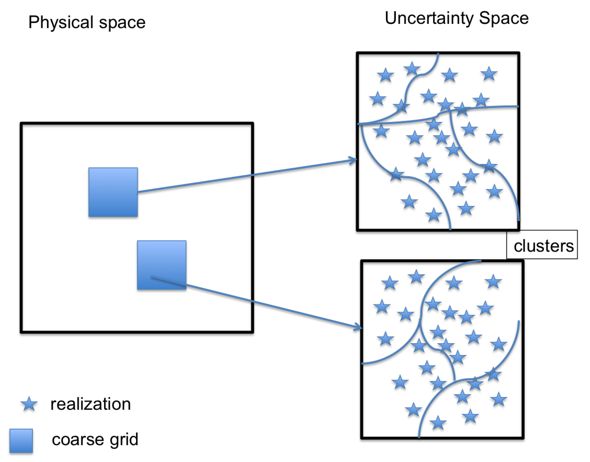
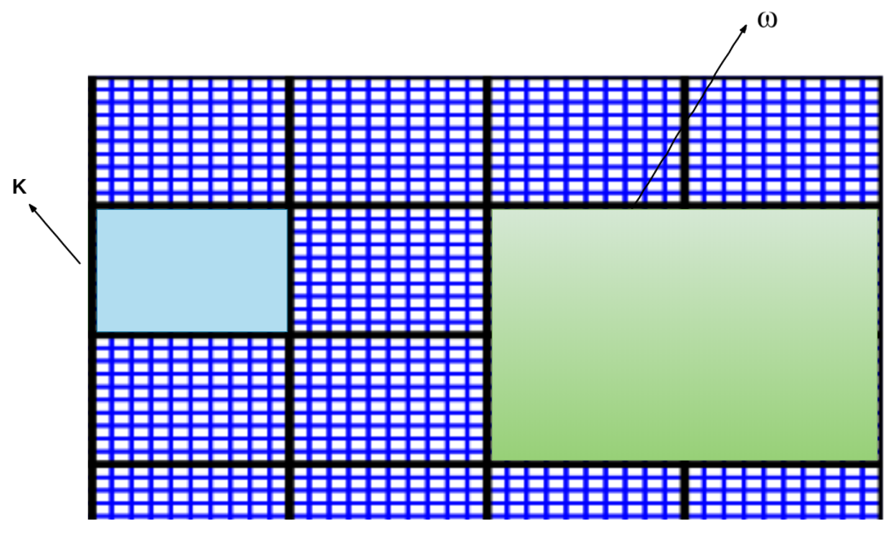
2.1. The Coarsening of the Parameter Space. The Main Idea
2.2. Space Coarsening—Generalized Multiscale Finite Element Method
2.2.1. Snapshot Space
2.2.2. Offline Spaces
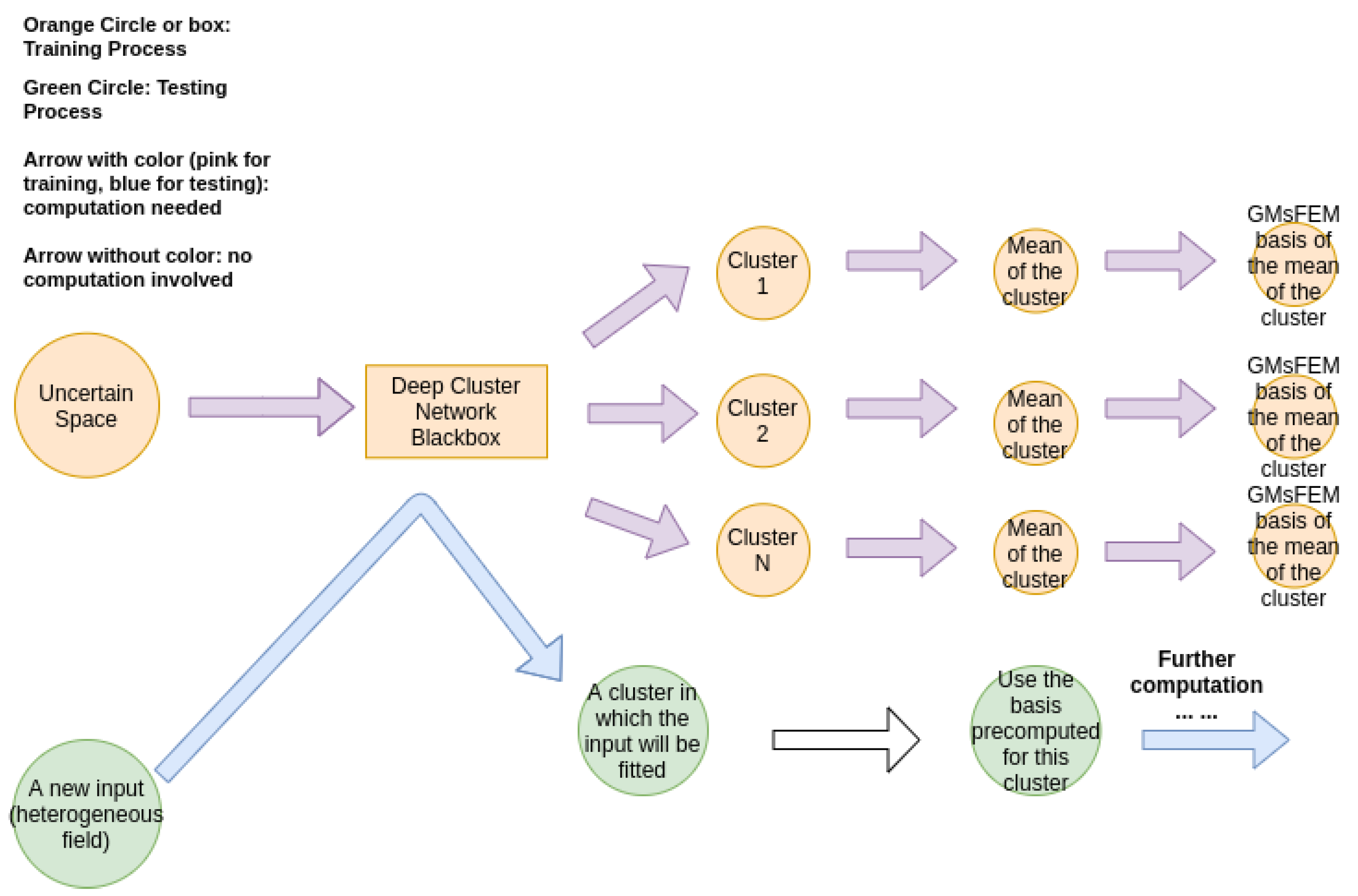
2.3. The Idea of the Proposed Method
- (Training) For a given input local neighborhood , we train the cluster (which will be detailed in next section) of the parameter space and get the clusters , where n is the number of clusters and is uniform for all j. Please note that we may have different cluster assignments in different local neighborhoods.
- (Training) For each local neighborhood and cluster , define the average and compute generalized multiscale basis for .
- (Testing) Given a new and for each local neighborhood , fit into a by the trained network (step 1) and use the pre-computed GMsFEM basis (step 2) to find the solution.
3. Deep Learning
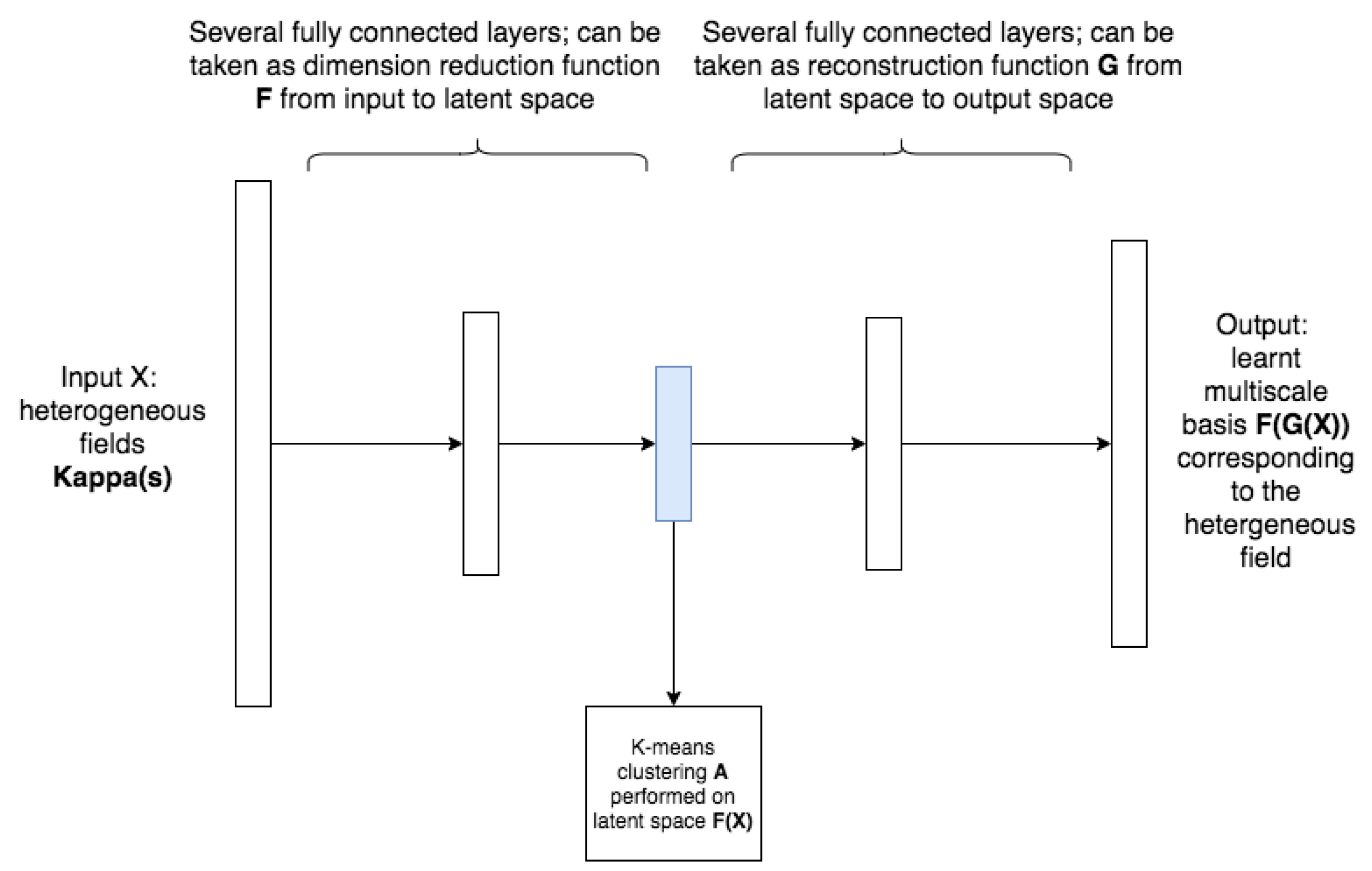
3.1. Clustering Net
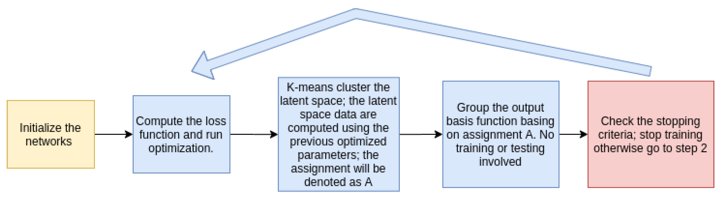
- Initialize the networks and clustering the output basis function.
- Compute the loss function L (defined later) and run optimization.
- Cluster the latent space by K-means algorithm (reduced dimension space, which is a middle layer of the cluster network); the latent space data are computed using the previous optimized parameters; the assignment will be denoted as A.
- Basis functions whose corresponding inputs are in the same cluster (basing on assignment A) will be grouped together. No training or fitting-in involved in this step.
- Repeat step 2 to step 4 until the stopping criteria is met.
3.2. Loss Functions
- Clustering loss : this is the mean standard deviation of all clusters of the learned basis and is the parameters we need to optimize. It should be noted that the loss here is computed using the learned basis instead of the input of the network. This loss controls the clustering process, i.e., the smaller the loss, the better the clustering in the sense of clustering the multiscale basis. Let us denote as jth realization in ith cluster; will then be jth learned basis in cluster i and let and be the parameters associated with G and F, the loss is then defined as follow,where is the number of clusters which is a hyper parameter and denotes the number of elements in cluster i; is the mean of cluster i. This loss clearly serves the purpose of clustering the solution instead of the input heterogeneous fields; however, in order to guarantee the learned basis are closed to the pre-computed multiscale basis, we need to define the reconstruction loss which measures the difference between the learned basis and the pre-computed basis.
- Reconstruction loss : this is the mean square error of multiscale basis , where m is the number of samples. This loss controls the construction process, i.e., if the loss is small, the learned basis are close to the real multiscale basis. This loss will supervise the learning of the cluster. It is defined as follow:where and are learned and pre-computed multiscale basis of ith sample separately.
3.3. Adversary Network Severing as an Additional Loss
4. Numerical Experiments
4.1. High Contrast Heterogeneous Fields with Moving Channels
4.2. Results
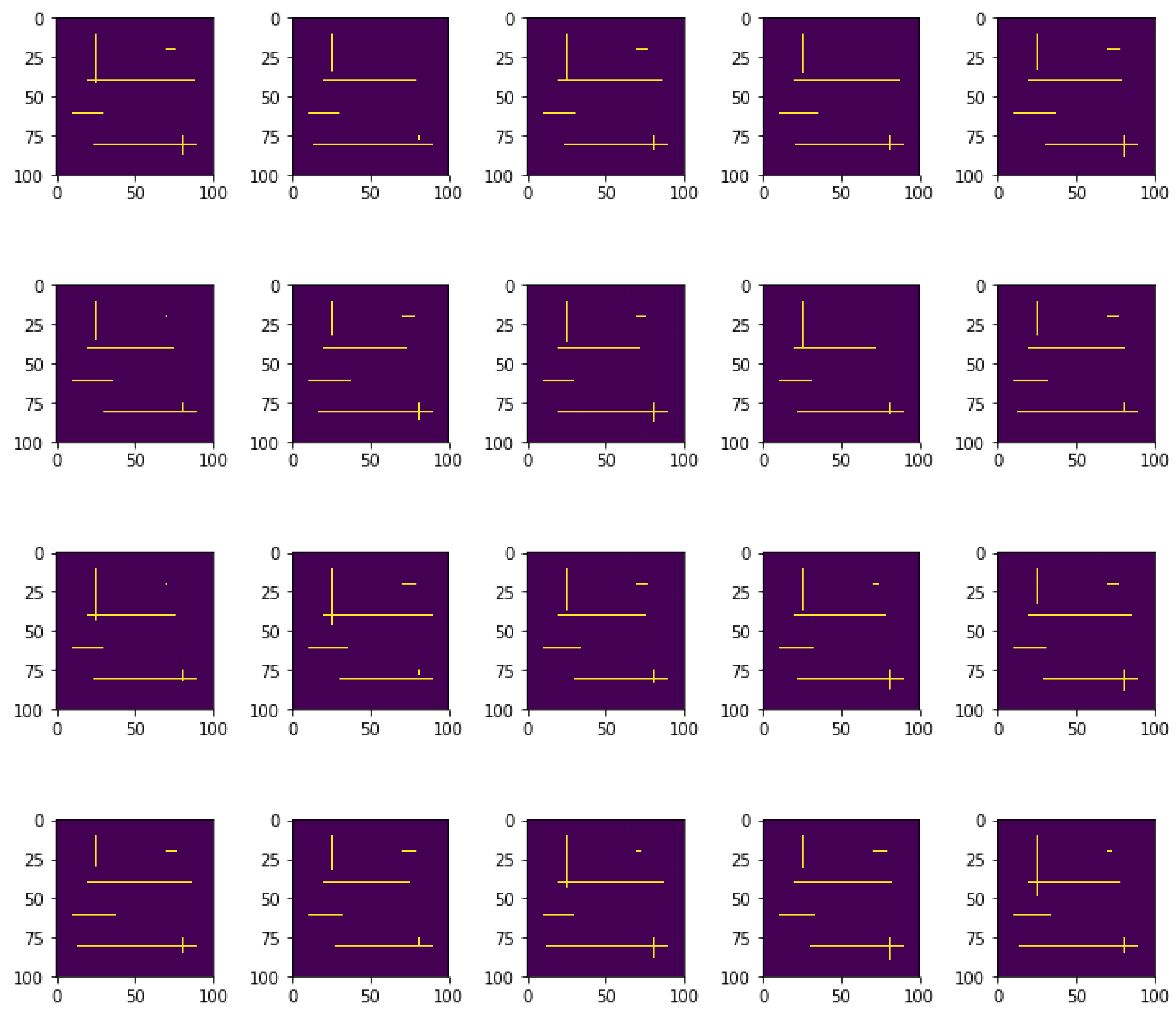
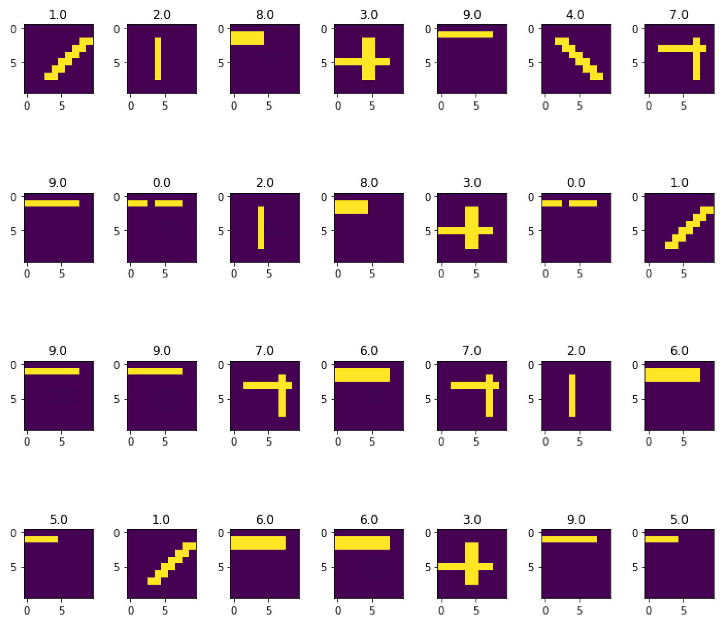
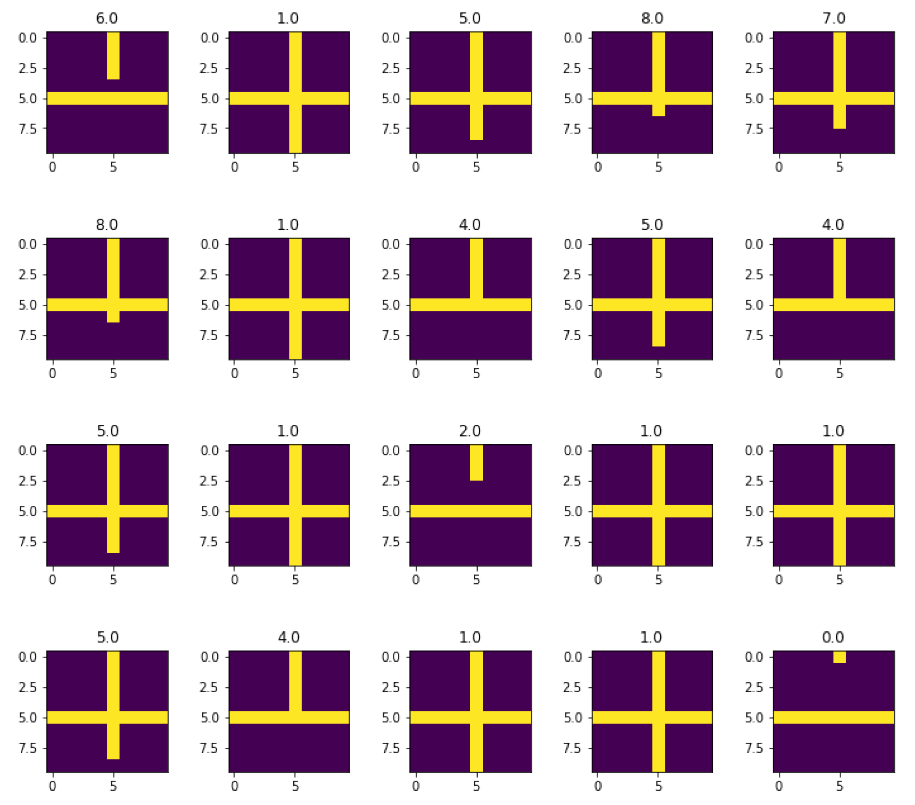
4.2.1. Cluster Assignment in a Local Coarse Element
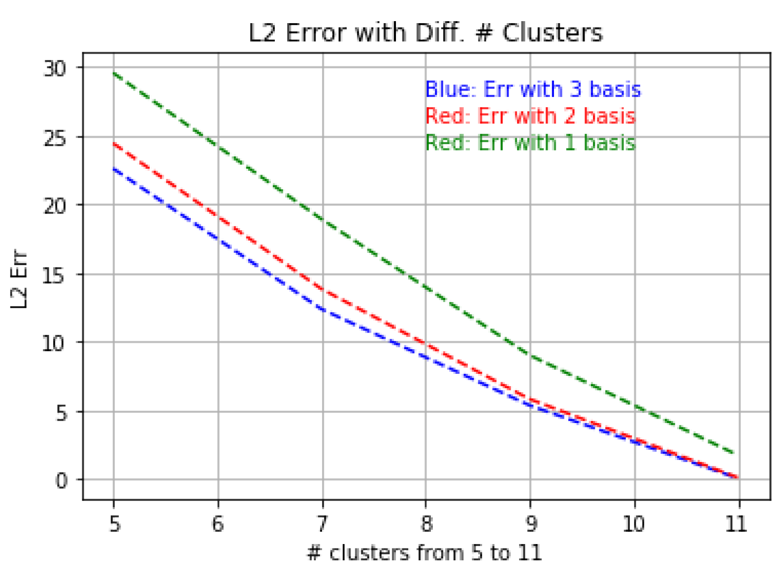
4.2.2. Relation of Error and the Number of Clusters
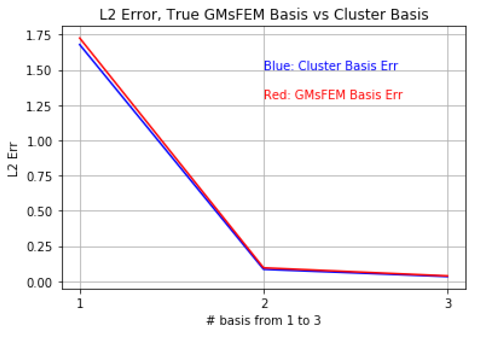
4.2.3. Comparison of Cluster-Based Method with Tradition Method
4.3. Effect of the Adversary Net
5. Conclusions
Author Contributions
Funding
Conflicts of Interest
References
- Tsiropoulou, E.; Koukas, K.; Papavassiliou, S. A socio-physical and mobility-aware coalition formation mechanism in public safety networks. EAI Endorsed Trans. Future Internet 2018, 4, 154176. [Google Scholar] [CrossRef]
- Thai, M.T.; Wu, W.; Xiong, H. Big Data in Complex and Social Networks; CRC Press: Boca Raton, FL, USA, 2016. [Google Scholar]
- Calo, V.M.; Efendiev, Y.; Galvis, J.; Ghommem, M. Multiscale empirical interpolation for solving nonlinear PDEs. J. Comput. Phys. 2014, 278, 204–220. [Google Scholar] [CrossRef] [Green Version]
- Chung, E.T.; Efendiev, Y.; Leung, W.T. Residual-driven online generalized multiscale finite element methods. J. Comput. Phys. 2015, 302, 176–190. [Google Scholar] [CrossRef] [Green Version]
- Chung, E.T.; Efendiev, Y.; Leung, W.T. An online generalized multiscale discontinuous Galerkin method (GMsDGM) for flows in heterogeneous media. Commun. Comput. Phys. 2017, 21, 401–422. [Google Scholar] [CrossRef]
- Chung, E.T.; Efendiev, Y.; Li, G. An adaptive GMsFEM for high-contrast flow problems. J. Comput. Phys. 2014, 273, 54–76. [Google Scholar] [CrossRef] [Green Version]
- Chung, E.T.; Efendiev, Y.; Li, G.; Vasilyeva, M. Generalized multiscale finite element methods for problems in perforated heterogeneous domains. Appl. Anal. 2016, 95, 2254–2279. [Google Scholar] [CrossRef] [Green Version]
- Efendiev, Y.; Galvis, J.; Lazarov, R.; Moon, M.; Sarkis, M. Generalized multiscale finite element method. Symmetric interior penalty coupling. J. Comput. Phys. 2013, 255, 1–15. [Google Scholar] [CrossRef] [Green Version]
- Efendiev, Y.; Galvis, J.; Li, G.; Presho, M. Generalized multiscale finite element methods: Oversampling strategies. Int. J. Multiscale Comput. Eng. 2014, 12, 465–484. [Google Scholar] [CrossRef]
- Chung, E.; Efendiev, Y.; Hou, T.Y. Adaptive multiscale model reduction with generalized multiscale finite element methods. J. Comput. Phys. 2016, 320, 69–95. [Google Scholar] [CrossRef] [Green Version]
- Chung, E.; Efendiev, Y.; Fu, S. Generalized multiscale finite element method for elasticity equations. Int. J. Geomath. 2014, 5, 225–254. [Google Scholar] [CrossRef] [Green Version]
- Chung, E.; Vasilyeva, M.; Wang, Y. A conservative local multiscale model reduction technique for Stokes flows in heterogeneous perforated domains. J. Comput. Appl. Math. 2017, 321, 389–405. [Google Scholar] [CrossRef] [Green Version]
- Chung, E.T.; Efendiev, Y.; Leung, W.T.; Zhang, Z. Cluster-based generalized multiscale finite element method for elliptic PDEs with random coefficients. J. Comput. Phys. 2018, 371, 606–617. [Google Scholar] [CrossRef] [Green Version]
- Karhunen, K. Über Lineare Methoden in der Wahrscheinlichkeitsrechnung; Suomalainen Tiedeakatemia: Helsinki, Finland, 1947; Volume 37. [Google Scholar]
- Lloyd, S. Least squares quantization in PCM. IEEE Trans. Inf. Theory 1982, 28, 129–137. [Google Scholar] [CrossRef]
- Wang, Y.; Cheung, S.W.; Chung, E.T.; Efendiev, Y.; Wang, M. Deep multiscale model learning. J. Comput. Phys. 2020, 406, 109071. [Google Scholar] [CrossRef] [Green Version]
- Wang, M.; Cheung, S.W.; Leung, W.T.; Chung, E.T.; Efendiev, Y.; Wheeler, M. Reduced-order deep learning for flow dynamics. The interplay between deep learning and model reduction. J. Comput. Phys. 2020, 401, 108939. [Google Scholar] [CrossRef]
- Vasilyeva, M.; Leung, W.T.; Chung, E.T.; Efendiev, Y.; Wheeler, M. Learning macroscopic parameters in nonlinear multiscale simulations using nonlocal multicontinua upscaling techniques. arXiv 2019, arXiv:1907.02921. [Google Scholar] [CrossRef] [Green Version]
- Cheung, S.W.; Chung, E.T.; Efendiev, Y.; Gildin, E.; Wang, Y.; Zhang, J. Deep global model reduction learning in porous media flow simulation. Comput. Geosci. 2020, 24, 261–274. [Google Scholar] [CrossRef]
- Wang, M.; Cheung, S.W.; Chung, E.T.; Efendiev, Y.; Leung, W.T.; Wang, Y. Prediction of discretization of gmsfem using deep learning. Mathematics 2019, 7, 412. [Google Scholar] [CrossRef] [Green Version]
- Goodfellow, I.; Bengio, Y.; Courville, A. Deep Learning; MIT Press: Cambridge, MA, USA, 2016. [Google Scholar]
- Caron, M.; Bojanowski, P.; Joulin, A.; Douze, M. Deep clustering for unsupervised learning of visual features. In Proceedings of the European Conference on Computer Vision (ECCV), Munich, Germany, 8–14 September 2018; pp. 132–149. [Google Scholar]
- Xie, J.; Girshick, R.; Farhadi, A. Unsupervised deep embedding for clustering analysis. In Proceedings of the International Conference on Machine Learning, New York, NY, USA, 19–24 June 2016; pp. 478–487. [Google Scholar]
- Yang, B.; Fu, X.; Sidiropoulos, N.D.; Hong, M. Towards k-means-friendly spaces: Simultaneous deep learning and clustering. In Proceedings of the 34th International Conference on Machine Learning-Volume 70. JMLR.org, Sydney, Australia, 6–11 August 2017; pp. 3861–3870. [Google Scholar]
- Bishop, C.M. Pattern Recognition and Machine Learning; Springer: Berlin, Germany, 2006. [Google Scholar]
- Isola, P.; Zhu, J.Y.; Zhou, T.; Efros, A.A. Image-to-image translation with conditional adversarial networks. In Proceedings of the IEEE Conference on Computer Vision and Pattern Recognition, Honolulu, HI, USA, 21–26 July 2017; pp. 1125–1134. [Google Scholar]
- Ledig, C.; Theis, L.; Huszár, F.; Caballero, J.; Cunningham, A.; Acosta, A.; Aitken, A.; Tejani, A.; Totz, J.; Wang, Z.; et al. Photo-realistic single image super-resolution using a generative adversarial network. In Proceedings of the IEEE Conference on Computer Vision and Pattern Recognition, Honolulu, HI, USA, 21–26 July 2017; pp. 4681–4690. [Google Scholar]
- Lai, W.S.; Huang, J.B.; Ahuja, N.; Yang, M.H. Deep laplacian pyramid networks for fast and accurate super-resolution. In Proceedings of the IEEE Conference on Computer Vision and Pattern Recognition, Honolulu, HI, USA, 21–26 July 2017; pp. 624–632. [Google Scholar]
- Johnson, J.; Alahi, A.; Fei-Fei, L. Perceptual losses for real-time style transfer and super-resolution. In Proceedings of the European Conference on Computer Vision, Amsterdam, The Netherlands, 11–14 October 2016; Springer: Berlin, Germany, 2016; pp. 694–711. [Google Scholar]
- Dong, C.; Loy, C.C.; He, K.; Tang, X. Image super-resolution using deep convolutional networks. IEEE Trans. Pattern Anal. Mach. Intell. 2015, 38, 295–307. [Google Scholar] [CrossRef] [Green Version]
- Kim, J.; Kwon Lee, J.; Mu Lee, K. Accurate image super-resolution using very deep convolutional networks. In Proceedings of the IEEE Conference on Computer Vision and Pattern Recognition, Las Vegas, NV, USA, 26 June–1 July 2016; pp. 1646–1654. [Google Scholar]
- Zhang, Y.; Li, K.; Li, K.; Wang, L.; Zhong, B.; Fu, Y. Image super-resolution using very deep residual channel attention networks. In Proceedings of the European Conference on Computer Vision (ECCV), Munich, Germany, 8–14 September 2018; pp. 286–301. [Google Scholar]
- Zhang, Y.; Tian, Y.; Kong, Y.; Zhong, B.; Fu, Y. Residual dense network for image super-resolution. In Proceedings of the IEEE Conference on Computer Vision and Pattern Recognition, Salt Lake City, UT, USA, 18–22 June 2018; pp. 2472–2481. [Google Scholar]
- Tai, Y.; Yang, J.; Liu, X. Image super-resolution via deep recursive residual network. In Proceedings of the IEEE Conference on Computer Vision and Pattern Recognition, Honolulu, HI, USA, 21–26 July 2017; pp. 3147–3155. [Google Scholar]
- Lim, B.; Son, S.; Kim, H.; Nah, S.; Mu Lee, K. Enhanced deep residual networks for single image super-resolution. In Proceedings of the IEEE Conference on Computer Vision and Pattern Recognition Workshops, Honolulu, HI, USA, 21–26 July 2017; pp. 136–144. [Google Scholar]
- Tai, Y.; Yang, J.; Liu, X.; Xu, C. Memnet: A persistent memory network for image restoration. In Proceedings of the IEEE International Conference on Computer Vision, Venice, Italy, 22–29 October 2017; pp. 4539–4547. [Google Scholar]
- Goodfellow, I.; Pouget-Abadie, J.; Mirza, M.; Xu, B.; Warde-Farley, D.; Ozair, S.; Courville, A.; Bengio, Y. Generative adversarial nets. In Proceedings of the Advances in Neural Information Processing Systems, Montreal, QC, Canada, 8–13 December 2014; pp. 2672–2680. [Google Scholar]
- Hu, J.; Shen, L.; Sun, G. Squeeze-and-excitation networks. In Proceedings of the IEEE Conference on Computer Vision and Pattern Recognition, Salt Lake City, UT, USA, 18–22 June 2018; pp. 7132–7141. [Google Scholar]
- Zhang, H.; Goodfellow, I.; Metaxas, D.; Odena, A. Self-attention generative adversarial networks. arXiv 2018, arXiv:1805.08318. [Google Scholar]
- Long, J.; Shelhamer, E.; Darrell, T. Fully convolutional networks for semantic segmentation. In Proceedings of the IEEE Conference on Computer Vision and Pattern Recognition, Boston, MA, USA, 7–12 June 2015; pp. 3431–3440. [Google Scholar]
- Szegedy, C.; Ioffe, S.; Vanhoucke, V.; Alemi, A.A. Inception-v4, inception-resnet and the impact of residual connections on learning. In Proceedings of the Thirty-First AAAI Conference on Artificial Intelligence, San Francisco, CA, USA, 4–9 February 2017. [Google Scholar]
- Szegedy, C.; Vanhoucke, V.; Ioffe, S.; Shlens, J.; Wojna, Z. Rethinking the inception architecture for computer vision. In Proceedings of the IEEE Conference on Computer Vision and Pattern Recognition, Las Vegas, NV, USA, 26 June–1 July 2016; pp. 2818–2826. [Google Scholar]
- Badrinarayanan, V.; Kendall, A.; Cipolla, R. Segnet: A deep convolutional encoder-decoder architecture for image segmentation. IEEE Trans. Pattern Anal. Mach. Intell. 2017, 39, 2481–2495. [Google Scholar] [CrossRef] [PubMed]
- Noh, H.; Hong, S.; Han, B. Learning deconvolution network for semantic segmentation. In Proceedings of the IEEE International Conference on Computer Vision, Santiago, Chile, 11–18 December 2015; pp. 1520–1528. [Google Scholar]
- Huang, G.; Liu, Z.; Van Der Maaten, L.; Weinberger, K.Q. Densely connected convolutional networks. In Proceedings of the IEEE Conference on Computer Vision and Pattern Recognition, Honolulu, HI, USA, 21–26 July 2017; pp. 4700–4708. [Google Scholar]
- Efendiev, Y.; Galvis, J.; Hou, T.Y. Generalized multiscale finite element methods (GMsFEM). J. Comput. Phys. 2013, 251, 116–135. [Google Scholar] [CrossRef] [Green Version]
- Hou, T.Y.; Wu, X.H. A multiscale finite element method for elliptic problems in composite materials and porous media. J. Comput. Phys. 1997, 134, 169–189. [Google Scholar] [CrossRef] [Green Version]
- Jenny, P.; Lee, S.; Tchelepi, H.A. Multi-scale finite-volume method for elliptic problems in subsurface flow simulation. J. Comput. Phys. 2003, 187, 47–67. [Google Scholar] [CrossRef]
- Calo, V.M.; Efendiev, Y.; Galvis, J.; Li, G. Randomized oversampling for generalized multiscale finite element methods. Multiscale Model. Simul. 2016, 14, 482–501. [Google Scholar] [CrossRef] [Green Version]
- Vidal-Jordana, A.; Montalban, X. Multiple sclerosis: Epidemiologic, clinical, and therapeutic aspects. Neuroimaging Clin. 2017, 27, 195–204. [Google Scholar] [CrossRef]
- Simonyan, K.; Zisserman, A. Very deep convolutional networks for large-scale image recognition. arXiv 2014, arXiv:1409.1556. [Google Scholar]
- Odena, A.; Dumoulin, V.; Olah, C. Deconvolution and checkerboard artifacts. Distill 2016, 1, e3. [Google Scholar] [CrossRef]


© 2020 by the authors. Licensee MDPI, Basel, Switzerland. This article is an open access article distributed under the terms and conditions of the Creative Commons Attribution (CC BY) license (http://creativecommons.org/licenses/by/4.0/).
Share and Cite
Zhang, Z.; Chung, E.T.; Efendiev, Y.; Leung, W.T. Learning Algorithms for Coarsening Uncertainty Space and Applications to Multiscale Simulations. Mathematics 2020, 8, 720. https://doi.org/10.3390/math8050720
Zhang Z, Chung ET, Efendiev Y, Leung WT. Learning Algorithms for Coarsening Uncertainty Space and Applications to Multiscale Simulations. Mathematics. 2020; 8(5):720. https://doi.org/10.3390/math8050720
Chicago/Turabian StyleZhang, Zecheng, Eric T. Chung, Yalchin Efendiev, and Wing Tat Leung. 2020. "Learning Algorithms for Coarsening Uncertainty Space and Applications to Multiscale Simulations" Mathematics 8, no. 5: 720. https://doi.org/10.3390/math8050720