Angular Correlation Using Rogers-Szegő-Chaos

Abstract

Polynomial chaos expresses a probability density function (pdf) as a linear combination of basis polynomials. If the density and basis polynomials are over the same field, any set of basis polynomials can describe the pdf; however, the most logical choice of polynomials is the family that is orthogonal with respect to the pdf. This problem is well-studied over the field of real numbers and has been shown to be valid for the complex unit circle in one dimension. The current framework for circular polynomial chaos is extended to multiple angular dimensions with the inclusion of correlation terms. Uncertainty propagation of heading angle and angular velocity is investigated using polynomial chaos and compared against Monte Carlo simulation.

1. Introduction

Engineering is an imperfect science. Noisy measurements from sensors in state estimation [1,2], a constantly changing environment in guidance [3,4,5], and improperly actuated controls [6] are all major sources of error. The more these sources of error are understood, the better the final product will be. Ideally, every variable with some sort of uncertainty associated with it would be completely and analytically described with its probability density function (pdf). Unfortunately, even if this is feasible for the initialization of a random variable, its evolution through time rarely yields a pdf with an analytic form. If the pdf cannot be given in analytic form, then approximations and assumptions must be made.

In many cases, a random variable is quantified using only its first two moments—as with the unscented transform [7]—and a further assumption is that the distribution is Gaussian. In cases where the variable’s uncertainty is relatively small and the dynamics governing its evolution are not highly nonlinear, this is not necessarily a poor assumption. In these cases, the higher order moments are highly dependent on the first two moments; i.e., there is a minimal amount of unique information in the higher order moments. In contrast, if either the uncertainty is large or the dynamics become highly nonlinear, the higher order moments become less dependent on the first two moments and contain larger amounts of unique information. In this case, the error associated with using only the first two moments becomes significant [8,9].

One method of quantifying uncertainty that does not require an assumption of the random variable’s pdf is polynomial chaos expansion (PCE) [10,11,12,13,14]. PCE characterizes a random variable as a coordinate in a polynomial vector space. Useful deterministic information about the random variable lies in this coordinate, including the moments of the random variable [15]. The expression of the coordinate depends on the basis in which it is expressed. In the case of PCE, the bases are made up of polynomials that are chosen based on the assumed density of the random variable; however, any random variable can be represented using any basis [16]. It is strongly noted that assuming the density of the random variable simply eases computation; with enough computing power, any random variable can be quantified with any basis [17]. The most common basis polynomials are those that are orthogonal with respect to common pdfs, such as the Hermite-Gaussian and Jacobi-beta polynomial-pdf pairs.

Polynomial chaos has been used to quantify and propagate the uncertainty in nonlinear systems including fluid dynamics [18,19,20,21], orbital mechanics in multiple element spaces [22], and has been expanded to facilitate Gaussian mixture models [23]. While polynomial chaos has been well-studied for variables that exist in the n-dimensional space of real numbers (${\mathbb{R}}^n$), many variables do not lie in this field. The variables that are of concern in this paper are angular variables. When estimating an angular random variable, such as the true anomaly of a body in orbit or vehicle attitude, a common approach is to assume that the variable is approximately equal to its projection on ${\mathbb{R}}^n$ and use methods designed for variables on that space. When the uncertainty is very small, this approximation is relatively effective; however, as the uncertainty increases, this approximation becomes invalid. Recently, work on directional statistics has been incorporated into state estimation, providing a method for estimating angular random variables directly on the n-dimensional special orthogonal group (${\mathbb{S}}^n$) [24,25,26]. Recent work [27] has shown that polynomial chaos can be used to estimate the mean and variance of one-dimensional angular random variables and the set of equinoctial orbital elements elements [28]. In neither case was a correlation estimated that included an angular state.

The sections of this paper include a detailed discussion of orthogonal polynomials in Section 2, including those that are orthogonal on the unit circle and two of the more common circular pdfs. In Section 3 an overview of polynomial chaos is given as well as the extension that has been made to include angular random variables, including the correlation between two angles. Finally, in Section 4, numerical results are presented comparing the correlation between two angular random variables calculated using Monte Carlo and PCE.

2. Orthogonal Polynomials

Let ${\mathbb{V}}^n$ be an n-dimensional vector space. A basis of this vector space is the minimal set of vectors that spans the vector space. An orthogonal basis is a subset of bases consisting of exactly n basis vectors such that the inner product between any two basis vectors, ${\beta }_m$ and ${\beta }_n$, is proportional to the Kronecker delta (${\delta }_{mn}$). Given mathematically with angle brackets, this orthogonal inner product takes the following form:

$$\begin{array}{cc}\hfill \langle {\beta }_m,{\beta }_n\rangle & =c{\delta }_{mn},\hfill \end{array}$$

where m and n are part of the set of positive integers, including zero. In the event $c=1$, the set is termed orthonormal. The $i^{\mathrm{th}}$ standard basis vector of ${\mathbb{V}}^n$ is generally the $i^{\mathrm{th}}$ vector of the n-dimensional identity; however, there are infinitely many bases for each vector space. It should be noted that it is not a requirement that a basis be orthogonal, merely linearly independent; however, the use of non-orthogonal bases is practically unheard-of.

An element $\alpha \in \mathbb{V}$ can be expressed in terms of an ordered basis $\mathcal{B}=\{{\beta }_1,{\beta }_2,\cdots ,{\beta }_n\}$, as the linear combination

$$\begin{array}{cc}\hfill \alpha & =a_1{\beta }_1+a_2{\beta }_2+\cdots +a_n{\beta }_n,\hfill \end{array}$$

(1)

where $[a_1,a_2,\cdots ,a_n]$ is the coordinate of $\alpha$. While any set of independent vectors can be used as a basis, different bases can prove beneficial—possibly by making the system more intuitive or more mathematically straightforward. When expressing the state of a physical system, the selection of a coordinate frame is effectively choosing a basis for the inhabited vector space. Consider a satellite in orbit. If the satellite’s ground track is of high importance (such as weather or telecommunications satellites), an Earth-fixed frame would be ideal. However, in cases where a satellite’s actions are dictated by other space-based objects (such as proximity operations), a body-fixed frame would be ideal.

It is common to constrict the term vector space to the spaces that are easiest to visualize, most notably a Cartesian space, where the bases are vectors radiating from the origin at right angles. The term vector space is much more broad than this though. A vector space need only contain the zero element and be closed under both scalar addition and multiplication, which applies to much more than vectors.

Most notable in this work is the idea of a polynomial vector space. Let ${\mathbb{P}}^{n+1}$ be an $(n+1)$-dimensional vector space made up of all polynomials of positive degree n or less with standard basis $\mathcal{B}=\{1,x,\cdots ,x^n\}$. The inner product with respect to the function $\omega$ on the real-valued polynomial space is given by

$$\begin{array}{cc}\hfill {\langle f\left(x\right),g\left(x\right)\rangle }_{\omega \left(x\right)}& ={\int }_{\mathbb{S}}f\left(x\right)g\left(x\right)d\omega \left(x\right),\hfill \end{array}$$

where $\omega \left(x\right)$ is a non-decreasing function with support $\mathbb{S}$ and f and g are any two polynomials of degree n or less. A polynomial family $\mathrm{\Phi }\left(x\right)$ is a set of polynomials with monotonically increasing order that are orthogonal. The orthogonality condition is given mathematically as

$$\begin{array}{cc}\hfill {\langle {\varphi }_m\left(x\right),{\varphi }_n\left(x\right)\rangle }_{\omega \left(x\right)}& ={\int }_{\mathbb{S}}{\varphi }_m\left(x\right){\varphi }_n\left(x\right)d\omega \left(x\right)=0\hfill \end{array}$$

(2a)

$$\begin{array}{cc}\hfill {\langle {\varphi }_m^2\left(x\right)\rangle }_{\omega \left(x\right)}& ={\int }_{\mathbb{S}}{\varphi }_m\left(x\right){\varphi }_m\left(x\right)d\omega \left(x\right)=c,\hfill \end{array}$$

(2b)

where ${\varphi }_k\left(x\right)$ is the polynomial of order k, c is a constant, and $\mathbb{S}$ is the support of the non-decreasing function $\omega \left(x\right)$. Note that while polynomials of negative orders ($k<0$), referred to as Laurent polynomials, exist, they are not covered in this work.

The most commonly used polynomial families are categorized in the Askey scheme, which groups the polynomials based on the generalized hypergeometric function (${}_p{F}_q$) from which they are generated [29,30,31].

Table 1. Common Orthogonal Polynomials.

Type	Polynomial	Hypergeometric Series	Support	Weight Function/Distribution
Continuous	Legendre	${}_2{F}_1$	$[-1,1]$	Uniform
	Jacobi	${}_2{F}_1$	$[-1,1]$	Beta
	Laguerre	${}_1{F}_1$	$[0,\infty )$	Exponential
	Probabilists’ Hermite	${}_2{F}_0$	$(-\infty ,\infty )$	Normal
Discrete	Charlier	${}_2{F}_0$	$\{0,1,2,\cdots \}$	Poisson
	Meixner	${}_2{F}_1$	$\{0,1,2,\cdots \}$	Negative Binomial
	Krawtchouk	${}_2{F}_1$	$\{0,1,\cdots ,N\}$	Binomial
	Hahn	${}_3{F}_2$	$\{0,1,\cdots ,N\}$	Hypergeometric

lists some of the polynomial families, their support, the non-decreasing function they are orthogonal with respect to (commonly referred to as a weight function), and the hypergeometric function they can be written in terms of. For completeness, Table 1 lists both continuous and discrete polynomial groups; however, the remainder of this work only considers continuous polynomials.

2.1. Polynomials Orthogonal on the Unit Circle

While the Askey polynomials are useful in many applications, their standard forms place them in the polynomial ring $\mathbb{R}\left[x\right]$, or all polynomials with real-valued coefficients that are closed under polynomial addition and multiplication. These polynomials are orthogonal with respect to measures on the real line. In the event that a set of polynomials orthogonal with respect a measure on a curved interval (e.g., the unit circle) is desired, the Askey polynomials would be insufficient.

In [32], Szegő uses the connection between points on the unit circle and points on a finite real interval to develop polynomials that are orthogonal on the unit circle. Polynomials of this type are now known as Szegő polynomials. Since the unit circle is defined to have unit radius, every point can be described on a real interval of length $2\pi$ and mapped to the complex variable $\vartheta =e^{i\theta }$, where i is the imaginary unit. All use of the variable $\vartheta$ in the following corresponds to this definition. The orthogonality expression for the Szegő polynomials, ${\varphi }_k\left(\vartheta \right)$, is

$$\begin{array}{cc}\hfill {\langle {\varphi }_m\left(\vartheta \right),{\varphi }_n\left(\vartheta \right)\rangle }_{\omega \left(\theta \right)}=\frac{1}{2\pi }{\int }_{-\pi }^{\pi }{\varphi }_m\left(\vartheta \right)\overline{{\varphi }_n\left(\vartheta \right)}\omega \left(\theta \right)d\theta & ={\delta }_{mn},\hfill \end{array}$$

where $\overline{{\varphi }_n\left(\vartheta \right)}$ is the complex conjugate of ${\varphi }_n\left(\vartheta \right)$ and $\omega \left(\theta \right)$ is the monotonically increasing weight function over the support. Note that, as opposed to Equation (2a), the Kronecker delta is not scaled, implying all polynomials using Szegő’s formulation are orthonormal.

While the general formulation outlined by Szegő is cumbersome—requiring the calculation of Fourier coefficients corresponding to the weight function and large matrix determinants—it does provide a framework for developing a set of polynomials orthogonal with respect to any conceivable continuous weight function. In addition to the initial research done by Szegő, further studies have investigated polynomials orthogonal on the unit circle [33,34,35,36,37,38].

Fortunately, there exist some polynomial families that are given explicitly, such as the Rogers-Szegő polynomials. The Rogers-Szegő polynomials have been well-studied [39,40,41] and were developed by Szegő based on work done by Rogers over the q-Hermite polynomials. For a more detailed description of the relationship between the Askey scheme of polynomials and their q-analog, the reader is encouraged to reference [31,42].

The generating function for the Rogers-Szegő polynomials is given as

$$\begin{array}{cc}\hfill {\varphi }_n(\vartheta ;q)& =\sum _{k=0}^n{\left(\genfrac{}{}{0pt}{}{n}{k}\right)}_q{\vartheta }^k,\hfill \end{array}$$

(3)

where ${\left(\genfrac{}{}{0pt}{}{n}{k}\right)}_q$ is the q-binomial

$$\begin{array}{ccccccc}\hfill {\left(\genfrac{}{}{0pt}{}{n}{k}\right)}_q& =\frac{{(q;q)}_n}{{(q;q)}_k{(q;q)}_{n-k}}\hfill & \hfill & \hfill \mathrm{and}& \hfill & \hfill {(a;q)}_n& =\prod _{j=0}^{n-1}(1-a{q}^j).\hfill \end{array}$$

The weight function that satisfies the orthogonality condition of these polynomials is

$$\begin{array}{cc}\hfill \omega \left(\theta \right)& =\frac{1}{\sqrt{-2\pi ln\left(q\right)}}\sum _{j=-\infty }^{\infty }exp\left\{\frac{{(\theta +2\pi j)}^2}{2ln\left(q\right)}\right\}0<q<1.\hfill \end{array}$$

(4)

In addition to the generating function, a three-step recurrence [43] exists, which is given by

$$\begin{array}{cc}\hfill {\varphi }_{n+1}(\vartheta ;q)& =(1+\vartheta ){\varphi }_n(\vartheta ;q)-(1-q^n)\vartheta {\varphi }_{n-1}(\vartheta ;q).\hfill \end{array}$$

(5)

For convenience, the first five polynomials are:

$$\begin{array}{cc}\hfill {\varphi }_0& =1\hfill \\ \hfill {\varphi }_1& =\vartheta +1\hfill \\ \hfill {\varphi }_2& ={\vartheta }^2+(q+1)\vartheta +1\hfill \\ \hfill {\varphi }_3& ={\vartheta }^3+(q^2+q+1){\vartheta }^2+(q^2+q+1)\vartheta +1\hfill \\ \hfill {\varphi }_4& ={\vartheta }^4+(q+1)(q^2+1){\vartheta }^3+(q+1)(q^2+q+1){\vartheta }^2+(q+1)(q^2+1)\vartheta +1.\hfill \end{array}$$

As is apparent, the q-binomial term causes the coefficients to be symmetric, which eases computation, and additionally, the polynomials are naturally monic.

2.2. Distributions on the Unit Circle

With the formulation of polynomials orthogonal on the unit circle, the weight function $\omega \left(\theta \right)$ has been continuously mentioned but not specifically addressed. In the general case, the weight function can be any non-decreasing function; however, the most common polynomial families are those that are orthogonal with respect to well-known pdfs, such as the ones listed in Table 1. Because weight functions must exist over the same support as the corresponding polynomials, pdfs over the unit circle are required for polynomial orthogonal on the unit circle.

2.2.1. Von Mises Distribution

One of the most common distributions used in directional statistics is the von Mises/von Mises-Fisher distribution [44,45,46]. The von Mises distribution lies on ${\mathbb{S}}^1$ (the subspace of ${\mathbb{R}}^2$ containing all points that are unit distance from the origin), whereas the von Mises-Fisher distribution has extensions into higher dimensional spheres. The circular von Mises pdf is given as [24]

$$\begin{array}{cc}\hfill p_m(\theta ;\mu ,\kappa )& =\frac{e^{\kappa cos(\theta -\mu )}}{2\pi I_0\left(\kappa \right)},\hfill \end{array}$$

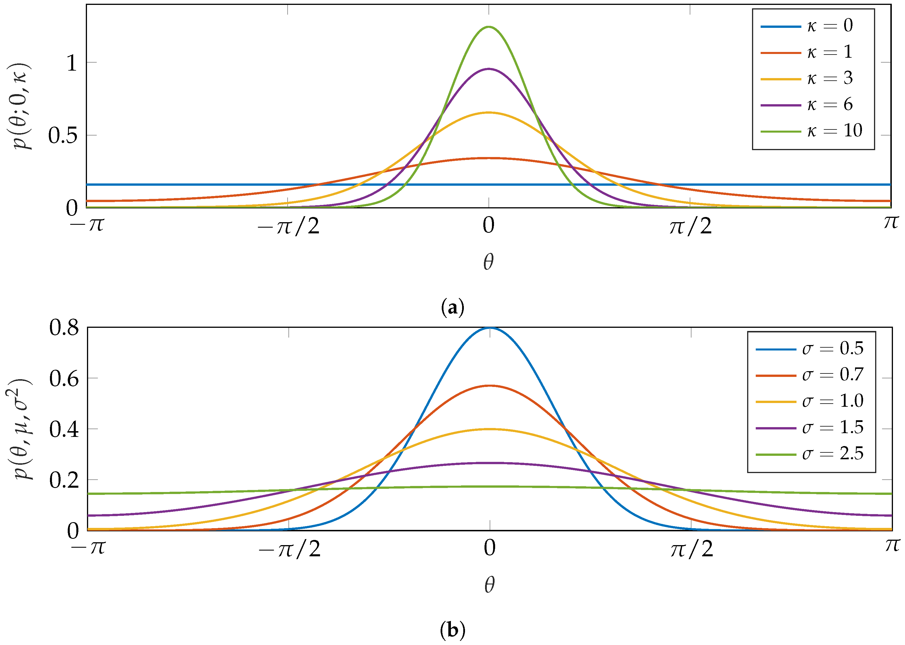
where $\mu$ is the mean angular direction on a $2\pi$ interval (usually $[-\pi ,\pi ]$), $\kappa \ge 0$ is a concentration parameter (similar to the inverse of the standard deviation), and $I_0$ is the zeroth order modified Bessel function of the first kind. The reason this distribution is so common is its close similarity to the normal distribution. This can be seen in Figure 1a, where von Mises distributions of various concentration parameters are plotted.

2.2.2. Wrapped Distributions

The easiest to visualize circular distribution, or rather group of distributions, that is discussed is the set of wrapped distributions. The wrapped distributions take a distribution on the real line and wrap it onto the unit circle according to

$$\begin{array}{cc}\hfill p_w\left(\theta \right)& =\sum _{j=-\infty }^{\infty }p(\theta +2\pi j),\hfill \end{array}$$

where the support of $p(·)$ is an interval of $\mathbb{R}$, and the domain of $p_w$ is an interval on $\mathbb{R}$ with length $2\pi$. For example, wrapping a normal distribution takes the pdf

$$\begin{array}{cc}\hfill p_n(x;\mu ,{\sigma }^2)& =\frac{1}{\sqrt{2\pi {\sigma }^2}}exp\left\{-\frac{{(x-\mu )}^2}{2{\sigma }^2}\right\},\hfill \end{array}$$

where the domain of x is $\mathbb{R}$, and $\mu$ and $\sigma$ are the mean and standard deviation, respectively, and wraps it, resulting in the wrapped pdf (in this case wrapped normal)

$$\begin{array}{cc}\hfill p_{wn}(\theta ;\mu ,{\sigma }^2)& =\frac{1}{\sqrt{2\pi {\sigma }^2}}\sum _{j=-\infty }^{\infty }exp\left\{-\frac{{(\theta -\mu +2\pi j)}^2}{2{\sigma }^2}\right\},\hfill \end{array}$$

where the domain of $\theta$ is an interval on $\mathbb{R}$ with length $2\pi$. Zero-mean normal distributions with varying values of $\sigma$ are wrapped, with the results shown in Figure 1b.

Recall the weight function of the Rogers-Szegő polynomials in Equation (4). As the log function is monotonically increasing, the term $log(1/q)$ increases monotonically as q decreases. Observing the extremes of q: as q approaches 1, $log(1/q)$ approaches 0, and as q approaches 0, $log(1/q)$ approaches ∞. Letting $log(1/q)={\sigma }^2$ and $\mu =0$, this becomes a zero-mean wrapped normal distribution.

It is clear from Figure 1 that both distributions described previously have strong similarities to the unwrapped normal distribution. Figure 1 also shows the difference in the standard deviation parameter. Whereas the wrapped normal distribution directly uses the standard deviation of the unwrapped distribution, the von Mises distribution is with respect to concentration parameter that is inversely related to the dispersion of the random variable. This makes the wrapped normal distribution slightly more intuitive when comparing with an unwrapped normal distribution.

2.2.3. Directional Statistics

The estimation of stochastic variables generally relies on calculating the statistics of that variable. Most notable of these statistics are the mean and variance, the first two central moments. For pdfs ($p\left(x\right)$) on the real line that are continuously integrable, the central moments are given as

$$\begin{array}{cc}{\mu }_1\hfill & ={\int }_{\mathbb{S}}xp\left(x\right)dx\hfill \\ {\mu }_k\hfill & ={\int }_{\mathbb{S}}{(x-{\mu }_1)}^{k}p\left(x\right)dxk\ge 2,\hfill \end{array}$$

(6)

where $\mathbb{S}$ is the support of $p\left(x\right)$. Although less utilized in general, raw moments are commonly used in directional statistics and are given as

$$\begin{array}{cc}\hfill {\rho }_k& ={\int }_{\mathbb{S}}{x}^{k}p\left(x\right)dx,\hfill \end{array}$$

or

$$\begin{array}{cc}\hfill {\rho }_k& ={\int }_{\mathbb{S}}{\vartheta }^{k}p\left(\theta \right)d\theta ,\hfill \end{array}$$

where the slight distinction is that the integration variable is within the variable $\vartheta =e^{i\theta }$. In addition, mean direction and circular variance are not the first and second central moments [24]. Instead, both are calculated from the first moment’s angle (${\theta }_1$) and length ($R_1$):

$$\begin{array}{rr}{\theta }_1& =\arg \left({\rho }_1\right)={tan}^{-1}\frac{\mathrm{imag}\left({\rho }_1\right)}{\mathrm{real}\left({\rho }_1\right)}\hfill \end{array}$$

(7a)

$$\begin{array}{ll}{R}_1& =\parallel {\rho }_1\parallel ,\end{array}$$

(7b)

where $\parallel ·\parallel$ is the $l^2$-norm. From Mardia [24], the length can be used to calculate the circular variance $V_1$ and circular standard deviation ${\sigma }_1$ according to

$$\begin{array}{cc}\hfill V_1& =1-R_1\hfill \end{array}$$

(8a)

$$\begin{array}{cc}\hfill {\sigma }_1& =\sqrt{-2\ln \left(R_1\right)}.\hfill \end{array}$$

(8b)

Effectively, as the length of the moment decreases, the concentration of the pdf about the mean direction decreases and the unwrapped standard deviation (USTD) increases. Note that while the subscript in Equations (7) and (8) is 1, there are corresponding mean directions and lengths associated with all moments; however, these are rarely used in applications.

3. Polynomial Chaos

At any given instance in time, the deviation of the estimate from the truth can be approximated as a Gaussian distribution centered at the mean of the estimate. The space of these mean-centered Gaussians is known as a Gaussian linear space [11]; when that space is closed (i.e., the distributions have finite second moments), it falls into the Gaussian Hilbert space $\mathcal{H}$. At this point, what is needed is a way to quantify $\mathcal{H}$, as this gives the uncertainty between the estimate and the truth. This can be achieved by projecting $\mathcal{H}$ onto a complete set of orthogonal polynomials when those basis functions are evaluated at a random variable $\xi \in \mathcal{H}$. While the distribution at any point in time natively exists in $\mathcal{H}$, its projection onto the set of orthogonal polynomials provides a way of quantifying it by means of the ordered coordinates, as in Equation (1).

The homogeneous chaos [10] specifies $\xi$ to be normally distributed with zero mean and unit variance (i.e., unit Gaussian), and the orthogonal polynomials to be the Hermite polynomials due to their orthogonality with respect to the standard Gaussian pdf [47]. Not only does this apply for Gaussian processes, but the Cameron-Martin theorem [48] says that this applies for any process with a finite second moment. Although the solution does converge as the number of orthogonal polynomials increases, further development has shown that, for different stochastic processes, certain basis functions cause the solution to converge faster [16], leading to the more general polynomial chaos (PC).

To begin applying this method mathematically for a general stochastic process, let a stochastic variable, $\epsilon$, be expressed as the linear combination over an infinite-dimensional vector space, i.e.,

$$\begin{array}{cc}\hfill \epsilon (x,\xi )& =\sum _{k=0}^{\infty }{ϵ}_k\left(x\right){\mathrm{\Psi }}_k\left(\xi \right),\hfill \end{array}$$

(9)

where ${ϵ}_i\left(x\right)$ is the deterministic component and ${\mathrm{\Psi }}_i\left(\xi \right)$ is an $i^{\mathrm{th}}$-order orthogonal basis function evaluated at, and orthogonal with respect to, the weight function, $\xi$. The polynomial families listed in Table 1 have been shown by Xiu [16] to provide convenient types of chaos based on their weight functions.

In general, the elements of the coordinate ($\left[ϵ\right]$) are called the polynomial chaos coefficients. These coefficients hold deterministic information about the distribution of the random variable; for instance, the first and second central moments of $\epsilon$ can be calculated easily as

$$\begin{array}{cc}\hfill \mathrm{E}\left[\epsilon \right]& ={\mu }_1={ϵ}_0\hfill \end{array}$$

(10a)

$$\begin{array}{cc}\hfill \mathrm{E}\left[{(\epsilon -\mathrm{E}\left[\epsilon \right])}^2\right]& ={\mu }_2=\sum _{k=1}^{\infty }{ϵ}_k^2{\langle {\mathrm{\Psi }}_k^2\rangle }_{p\left(\xi \right)},\hfill \end{array}$$

(10b)

where $\mathrm{E}\left[\right]$ denotes expected value.

Now, let $\mathit{\epsilon }$ be an n-dimensional vector. Each of the n elements in $\mathit{\epsilon }$ are expanded separately; therefore, Equation (9) is effectively identical in vector form

$$\begin{array}{cc}\hfill \mathit{\epsilon }(\mathit{x},\xi )& =\left[\begin{array}{c}{\epsilon }^{\left(1\right)}(x^{\left(1\right)},\xi )\\ {\epsilon }^{\left(2\right)}(x^{\left(2\right)},\xi )\\ ⋮\\ {\epsilon }^{\left(n\right)}(x^{\left(n\right)},\xi )\end{array}\right]=\left[\begin{array}{c}\sum _{k=0}^{\infty }{ϵ}_k^{\left(1\right)}\left(x^{\left(1\right)}\right){\mathrm{\Psi }}_k\left(\xi \right)\\ \sum _{k=0}^{\infty }{ϵ}_k^{\left(2\right)}\left(x^{\left(2\right)}\right){\mathrm{\Psi }}_k\left(\xi \right)\\ ⋮\\ \sum _{k=0}^{\infty }{ϵ}_k^{\left(n\right)}\left(x^{\left(n\right)}\right){\mathrm{\Psi }}_k\left(\xi \right)\end{array}\right].\hfill \end{array}$$

Because the central moments are independent, the mean and variance of each their calculations similarly do not change. In addition to mean and variance, the correlation between two random variables is commonly desired. With the chaos coefficients estimated for each random variable and the polynomial basis known, correlation terms such covariance can be estimated.

3.1. Covariance

Let the continuous variables a and b have chaos expansions

$$\begin{array}{ccccccc}\hfill a(x,\xi )& =\sum _{j=0}^{\infty }{\alpha }_j\left(x\right){\mathrm{\Psi }}_j\left(\xi \right)\hfill & \hfill & \hfill \mathrm{and}& \hfill & \hfill b(z,\zeta )& =\sum _{k=0}^{\infty }{\beta }_k\left(z\right){\mathrm{\Phi }}_k\left(\zeta \right).\hfill \end{array}$$

(11)

The covariance between a and b can be expressed in terms of two nested expected values

$$\begin{array}{cc}\hfill \mathrm{cov}(a,b)& =\mathrm{E}\left[\right(a-\mathrm{E}\left[a\right]\left)\right(b-\mathrm{E}\left[b\right]\left)\right],\hfill \end{array}$$

the external of which can be expressed as a double integral yielding

$$\begin{array}{cc}\hfill \mathrm{cov}(a,b)& ={\int }_{\mathbb{A}}{\int }_{\mathbb{B}}(a-\mathrm{E}\left[a\right])(b-\mathrm{E}\left[b\right])dbda,\hfill \end{array}$$

(12)

where $\mathbb{A}$ and $\mathbb{B}$ are the supports of a and b respectively. Substituting the expansions from Equation (11) into Equation (12) and acknowledging that the zeroth coefficient is the expected value gives

$$\begin{array}{ll}\mathrm{cov}(a,b)& ={\int }_{\mathbb{A}}{\int }_{\mathbb{B}}(ab-a\mathrm{E}\left[b\right]-b\mathrm{E}\left[a\right]+\mathrm{E}\left[a\right]\mathrm{E}\left[b\right])dbda\\ & ={\int }_{\mathbb{A}}{\int }_{\mathbb{B}}(ab-{\beta }_{0}a-{\alpha }_{0}b+{\alpha }_0{\beta }_0)dbda\\ & =-{\alpha }_0{\beta }_0+{\int }_{\mathbb{A}}{\int }_{\mathbb{B}}\left(ab\right)dbda\end{array}$$

(13a)

$$\begin{array}{rr}& =-{\alpha }_0{\beta }_0+{\int }_{\mathbb{X}}{\int }_{\mathbb{Z}}\sum _{j=0}^{\infty }{\alpha }_j\left(x\right){\mathrm{\Psi }}_j\left(\xi \right)\sum _{k=0}^{\infty }{\beta }_k\left(z\right){\mathrm{\Phi }}_k\left(\zeta \right)d\zeta d\xi .\end{array}$$

(13b)

Note the change of variables between Equations (13a) and (13b). This is possible because the random variable and the weight function ($a/\xi$ and $b/\zeta$ in this case) are over the same support. Additionally, the notation of the support variable is changed to be consistent with the integration variable.

As long as the covariance is finite, the summation and the integrals can be interchanged [49], giving a final generalized expression for the covariance to be

$$\begin{array}{cc}\hfill \mathrm{cov}(a,b)& =\sum _{j=1}^{\infty }\sum _{k=1}^{\infty }{\alpha }_j\left(x\right){\beta }_k\left(z\right){\int }_{\mathbb{X}}{\int }_{\mathbb{Z}}{\mathrm{\Psi }}_j\left(\xi \right){\mathrm{\Phi }}_k\left(\zeta \right)d\zeta d\xi .\hfill \end{array}$$

(14)

In general, no further simplifications can be made; however, if the variables x and z are expanded using the same set of basis polynomials, then integration reduces to

$$\begin{array}{cc}\hfill \mathrm{cov}(a,b)& =\sum _{k=1}^{\infty }\sum _{j=1}^{\infty }{\alpha }_k\left(x\right){\beta }_j\left(z\right){\int }_{\mathbb{X}}{\mathrm{\Psi }}_k\left(\xi \right){\mathrm{\Psi }}_j\left(\xi \right)p\left(\xi \right)d\xi ,\hfill \end{array}$$

(15)

containing a single variable with respect to the base pdf. Taking advantage of the basis polynomial orthogonality yields the following simple expression:

$$\begin{array}{cc}\hfill \mathrm{cov}(a,b)& =\sum _{k=1}^{\infty }{\alpha }_k\left(x\right){\beta }_k\left(z\right){\langle {\mathrm{\Psi }}_k^2\rangle }_{p\left(\xi \right)}.\hfill \end{array}$$

(16)

Combined with the variance, the covariance matrix of the $2\times 2$ system of x and z just discussed is given as

$$\begin{array}{cc}\hfill \mathit{P}& =\sum _{k=1}^{\infty }\left[\begin{array}{cc}{\alpha }_k^2& {\alpha }_k{\beta }_k\\ {\alpha }_k{\beta }_k& {\beta }_k^2\end{array}\right]{\langle {\mathrm{\Psi }}_k^2\rangle }_{p\left(\xi \right)}.\hfill \end{array}$$

For an n-dimensional state, let $\mathit{ϵ}$ be the $n\times \infty$ matrix for the n, theoretically infinite, chaos coefficients. Written generally, the covariance matrix in terms of a chaos expansion is

$$\begin{array}{cc}\hfill \mathit{P}& =\sum _{k=1}^{\infty }{\mathit{ϵ}}_k{\mathit{ϵ}}_k^T{\langle {\mathrm{\Psi }}_k^2\rangle }_{p\left(\xi \right)}.\hfill \end{array}$$

In cases where orthonormal polynomials are used, the polynomial inner product disappears completely leaving only the summation of the estimated chaos coefficients

$$\begin{array}{cc}\hfill \mathit{P}& =\sum _{k=1}^{\infty }{\mathit{ϵ}}_k{\mathit{ϵ}}_k^T.\hfill \end{array}$$

(17)

3.2. Coefficient Calculation

The two most common methods of solving Equation (9) for the chaos coefficients are sampling-based and projection-based. The first, and most common, approach requires truncating the infinite summation in Equation (9) to yield

$$\begin{array}{cc}\hfill \epsilon (x,\xi )& =\sum _{k=0}^N{ϵ}_k\left(x\right){\mathrm{\Psi }}_k\left(\xi \right),\hfill \end{array}$$

(18)

where the truncation term N, which depends on the dimension of the state n and the highest order polynomial p, is

$$\begin{array}{cc}\hfill N+1& =\frac{(n+p)!}{n!p!}.\hfill \end{array}$$

Drawing Q samples of $\xi$, where $Q>N$, and evaluating ${\mathrm{\Psi }}_k$ and $\epsilon$ at these points effectively results in randomly sampling $\epsilon$ directly. After initial sampling, $\epsilon$ can be transformed in x (commonly x is taken to be time so this indicates propagating the variable forward in time) resulting in a system of Q equations with $N+1$ unknowns that describe the pdf of $\epsilon$ after the transformation that is given by

$$\begin{array}{cc}\hfill \epsilon (x,{\xi }_1)& ={ϵ}_0\left(x\right){\mathrm{\Psi }}_0\left({\xi }_1\right)+{ϵ}_1\left(x\right){\mathrm{\Psi }}_1\left({\xi }_1\right)+\cdots +{ϵ}_N\left(x\right){\mathrm{\Psi }}_N\left({\xi }_1\right)\hfill \\ \hfill \epsilon (x,{\xi }_2)& ={ϵ}_0\left(x\right){\mathrm{\Psi }}_0\left({\xi }_2\right)+{ϵ}_1\left(x\right){\mathrm{\Psi }}_1\left({\xi }_2\right)+\cdots +{ϵ}_N\left(x\right){\mathrm{\Psi }}_N\left({\xi }_2\right)\hfill \\ \hfill & ⋮\hfill \\ \hfill \epsilon (x,{\xi }_Q)& ={ϵ}_0\left(x\right){\mathrm{\Psi }}_0\left({\xi }_Q\right)+{ϵ}_1\left(x\right){\mathrm{\Psi }}_1\left({\xi }_Q\right)+\cdots +{ϵ}_N\left(x\right){\mathrm{\Psi }}_N\left({\xi }_Q\right).\hfill \end{array}$$

This overdetermined system can be solved for $\mathit{ϵ}$ using a least-squares approximation. The coefficients can then be used to calculate convenient statistical data about $\epsilon$ (e.g., central and raw moments).

While the sampling-based method is more practical to apply, the projection based method is not dependent on sampling the underlying distribution. Projecting the pdf of $\epsilon$ onto the $j^{\mathrm{th}}$ basis yields

$$\begin{array}{cc}\hfill {〈\epsilon (x,\xi ),{\mathrm{\Psi }}_j\left(\xi \right)〉}_{p\left(\xi \right)}& ={〈\sum _{k=0}^{\infty }{ϵ}_k\left(x\right){\mathrm{\Psi }}_k\left(\xi \right),{\mathrm{\Psi }}_j\left(\xi \right)〉}_{p\left(\xi \right)}.\hfill \end{array}$$

The inner product is with respect to the variable $\xi$; therefore, the coefficient $ϵ$ acts as a scalar. The inner product is linear in the first argument; therefore, the summation coefficients can be removed from the inner product without alteration, that is

$$\begin{array}{cc}\hfill {〈\epsilon (x,\xi ),{\mathrm{\Psi }}_j\left(\xi \right)〉}_{p\left(\xi \right)}& =\sum _{k=0}^{\infty }{ϵ}_k\left(x\right){〈{\mathrm{\Psi }}_k\left(\xi \right),{\mathrm{\Psi }}_j\left(\xi \right)〉}_{p\left(\xi \right)}.\hfill \end{array}$$

(19)

In contrast, if the summation is an element of the second argument, the linearity condition still holds; however, the coefficients incur a complex conjugate. Recall the basis polynomials are generally chosen to be orthogonal, so the right-hand inner product of Equation (19) reduces to the scaled Kronecker delta, resulting in

$$\begin{array}{cc}\hfill {〈\epsilon (x,\xi ),{\mathrm{\Psi }}_j\left(\xi \right)〉}_{p\left(\xi \right)}& =\sum _{k=0}^{\infty }{ϵ}_k\left(x\right){〈{\mathrm{\Psi }}_k\left(\xi \right),{\mathrm{\Psi }}_j\left(\xi \right)〉}_{p\left(\xi \right)}\hfill \\ \hfill & =\sum _{k=0}^{\infty }{ϵ}_k\left(x\right)c{\delta }_{kj}.\hfill \end{array}$$

This leaves only the $j^{\mathrm{th}}$ term (with the constant $c={\langle {\mathrm{\Psi }}_j^2\left(\xi \right)\rangle }_{p\left(\xi \right)}$), and an equation that is easily solvable for ${ϵ}_j$ is

$$\begin{array}{cc}\hfill {ϵ}_j\left(x\right)& =\frac{{〈\epsilon (x,\xi ),{\mathrm{\Psi }}_j\left(\xi \right)〉}_{p\left(\xi \right)}}{{\langle {\mathrm{\Psi }}_j^2\left(\xi \right)\rangle }_{p\left(\xi \right)}}\hfill \end{array}$$

(20a)

$$\begin{array}{cc}\hfill & =\frac{{\int }_{\mathbb{Z}}\epsilon (x,\xi ){\mathrm{\Psi }}_j\left(\xi \right)dp\left(\xi \right)}{{\int }_{\mathbb{Z}}{\mathrm{\Psi }}_j^2\left(\xi \right)dp\left(\xi \right)},\hfill \end{array}$$

(20b)

which almost always requires numeric approximation.

3.3. Implementation Procedure

For convenience, the procedure for estimating the mean and covariance of a random state is given in Algorithm 1. Let $\mathit{\epsilon }$ be the state of a system with uncertainty defined by mean $\mathit{m}$ and covariance $\mathit{P}$ subject to a set of system dynamics over the time vector T. The algorithm outlines the steps required to estimate the mean and covariance of the state after the amount of time specified by T.

Algorithm 1 Estimation of mean and covariance using a polynomial chaos expansion.

1: procedurePCE_EST(${\mathit{m}}_0,{\mathit{P}}_0$)           ▹ Estimation of $\mathit{m}$ and $\mathit{P}$ using PCE   2:   for $k=1$ to T do   3:         Draw samples of $\xi$ based on chaos type       ▹ Either randomly or intelligently   4:         ${\mathit{\epsilon }}_{k-1}\leftarrow {\mathit{m}}_{k-1},{\mathit{P}}_{k-1},\xi$                  ▹ Sample $\mathit{\epsilon }$ based on $\xi$   5:         ${\mathit{\epsilon }}_k$ from propagating $\mathit{\epsilon }$ based on state dynamics   6:         $\mathit{ϵ}\leftarrow$Equation (20a)   7:         ${\mathit{m}}_k\leftarrow$Equation (10a)   8:         ${\mathit{P}}_k\leftarrow$Equation (17)   9:    end for 10:   return $\mathit{m},\mathit{P}$ 11: end procedure

3.4. Complex Polynomial Chaos

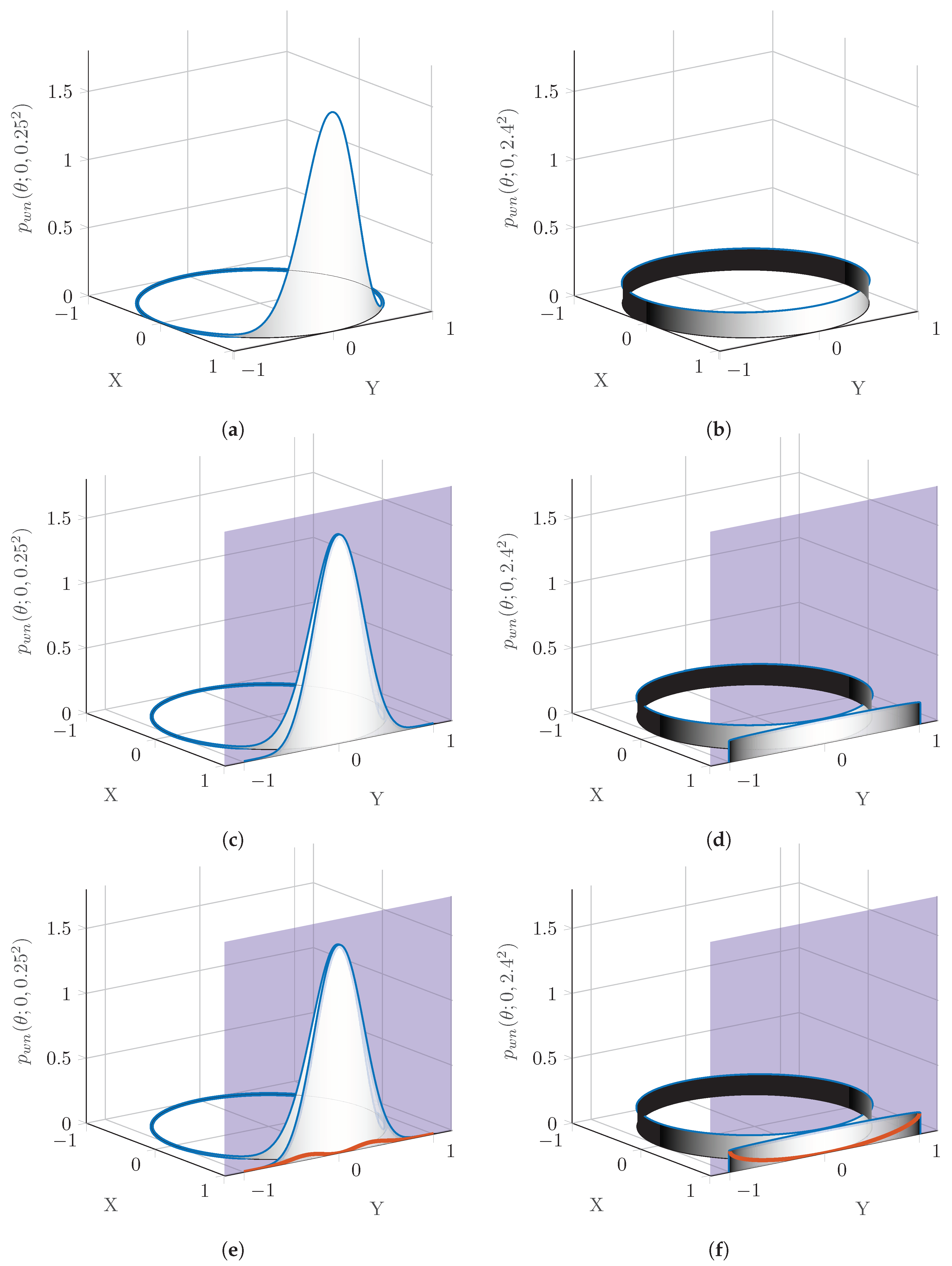
While polynomial chaos has been well-studied and applied to a various number of applications in ${\mathbb{R}}^n$, alterations must be made for the restricted space ${\mathbb{S}}^n$ due to its circular nature. A linear approximation can be made with little error when a circular variable’s uncertainty is small; however, as the uncertainty increases, the linearization can impose significant error. Figure 2 shows the effects of projecting two wrapped normal distributions with drastically different standard deviations onto a tangent plane. The two wrapped normal distributions are shown in Figure 2a,b, with USTDs of $0.25$ and $0.4$ rad, respectively. Clearly, even relatively small USTDs result in approximately uniform wrapped pdfs.

One of the most basic projections is an orthogonal projection from an n-dimensional space onto an $n-1$ dimensional plane. In this case, the wrapped normal pdf is projected orthogonally onto the plane $(1,x,z)$, which lies tangent to the unit circle at the point (1,0), coinciding with the mean direction of both pdfs. The plane, and the projection of the pdf onto this plane are shown in Figure 2c,d. Approximating the circular pdf as the projected planar pdf comes with an associated loss of information. At the tangent point, there is obviously no information loss; however, when the physical distance from the original point to the projected point is considered, the error associated with the projected point increases. As is the case with many projection methods concerning circular and spherical bodies, all none of the information from the far side of the body is available in the projection. The darkness of the shading in all of Figure 2 comes from the distance of the projection where white is no distance, and black is a distance value of least one (implying the location is on the hemisphere directly opposite the mean direction).

To better indicate the error induced by this type of projection, Figure 2e,f also include a measure that shows how far the pdf has been projected as a percentage of the overall probability at a given point. At the tangent point, there is no projection required, therefore the circular pdf has to be shifted $0\%$ in the x direction. As the pdf curves away from the tangent plane, the pdf has to be projected farther. The difference between Figure 2e and Figure 2f is that the probability approaches zero nearing $y=\pm 1$ in Figure 2e; therefore, the effect of the error due to projection is minimal. In cases where the information is closely concentrated about one point, tangent plane projections can be good assumptions. Contrarily, in Figure 2f the pdf does not approach zero, and therefore the approximation begins to become invalid. Accordingly, the red error line approaches the actual pdf, indicating that the majority of the pdf has been significantly altered in the projection.

In addition to restricting the space to the unit circle, most calculations required when dealing with angles take place in the complex field. In truth, the bulk of expanding polynomial chaos to be suitable for angular random variables is generalizing it to complex vector spaces. Previous work by the authors [27] has shown that a stochastic angular random variable can be expressed using a polynomial chaos expansion. Specifically, the chaos expansion is one that uses polynomials that are orthogonal with respect to probability measures on the complex unit circle as opposed to the real line.

3.5. Szegő-Chaos

For the complex angular case, the chaos expansion is transformed slightly, such that

$$\begin{array}{cc}\hfill \epsilon (x,\vartheta )& =\sum _{k=0}^{\infty }{ϵ}_k\left(x\right)\overline{{\mathrm{\Psi }}_k\left(\vartheta \right)},\hfill \end{array}$$

(21)

where, once again, $\vartheta =e^{i\theta }$. The complex conjugate is not required in Equation (21), but it must be remembered that the expansion must be projected onto the conjugate of the expansion basis in Equation (20b). While ultimately a matter of choice, it is more convenient to express the expansion in terms of the conjugate basis, rather than the original basis.

Unfortunately, while the first moment is calculated the same for real and complex valued polynomials, the real valued process does not extend to complex valued polynomials. This is because of the slightly different orthogonality condition between real and complex valued polynomials. While the inner product given in Equation (2a) is not incorrect, it is only valid for real valued polynomials. The true inner product of two functions contains a complex conjugate, that is

$$\begin{array}{cc}\hfill {\langle {\mathrm{\Psi }}_m,{\mathrm{\Psi }}_n\rangle }_{p\left(x\right)}& ={\int }_{\mathbb{X}}{\mathrm{\Psi }}_m\left(x\right)\overline{{\mathrm{\Psi }}_n\left(x\right)}p\left(x\right)dx=c{\delta }_{mn}.\hfill \end{array}$$

The difference between $\mathbb{R}\left[x\right]$ and $\mathbb{C}\left[x\right]$ is that the complex conjugate has no effect on $\mathbb{R}\left[x\right]$. Fortunately, the zeroth polynomial of the Szegő polynomials is unitary just like the Askey polynomials. The complex conjugate has no effect; therefore the zeroth polynomial has no imaginary component and is calculated the same for complex and purely real valued random variables.

The complex conjugate of a real valued function has no effect; therefore, the first moment takes the form;

$$\begin{array}{cc}\hfill {\mu }_1& =\sum _{k=0}^{\infty }{ϵ}_k\left(x\right){\int }_{\mathbb{X}}{\mathrm{\Psi }}_k\left(\xi \right){\mathrm{\Psi }}_0\left(\xi \right)p\left(\xi \right)d\xi =\sum _{k=0}^{\infty }{ϵ}_k\left(x\right){\int }_{\mathbb{X}}{\mathrm{\Psi }}_k\left(\xi \right)\overline{{\mathrm{\Psi }}_0\left(\xi \right)}p\left(\xi \right)d\xi .\hfill \end{array}$$

(22)

In general, calculation of the second raw moment and the covariance cannot be simplified beyond

$$\begin{array}{cc}\hfill {\mu }_2& =\sum _{j=0}^{\infty }\sum _{k=0}^{\infty }{ϵ}_j{ϵ}_k{\int }_{\mathbb{X}}\overline{{\mathrm{\Psi }}_j\left(\xi \right)}\overline{{\mathrm{\Psi }}_k\left(\xi \right)}p\left(\xi \right)d\xi \hfill \\ \hfill & =\sum _{j=0}^{\infty }\sum _{k=0}^{\infty }{ϵ}_j{ϵ}_k{〈\overline{{\mathrm{\Psi }}_j\left(\xi \right)},{\mathrm{\Psi }}_k\left(\xi \right)〉}_{p\left(\xi \right)}\hfill \end{array}$$

(23)

$$\mathrm{cov}(x,z)=\sum _{j=1}^{\infty }\sum _{k=1}^{\infty }{\alpha }_j{\beta }_k{\int }_{\mathbb{X}}{\int }_{\mathbb{Z}}\overline{{\mathrm{\Psi }}_j\left(\zeta \right){\mathrm{\Phi }}_k\left(\xi \right)}p(\zeta ,\xi )d\zeta d\xi .$$

(24)

The simplification from Equation (14) to Equation (15) as a result of shared bases can similarly be applied to Equation (24). This simplifies Equation (24) to a double summation but only a singular inner product (i.e., integral), i.e.,

$$\begin{array}{cc}\hfill \mathrm{cov}(x,z)& =\sum _{j=1}^{\infty }\sum _{k=1}^{\infty }{\alpha }_j{\beta }_k{\int }_{\mathbb{X}}\overline{{\mathrm{\Psi }}_j\left(\xi \right){\mathrm{\Psi }}_k\left(\xi \right)}p\left(\xi \right)d\xi \hfill \\ \hfill & =\sum _{j=1}^{\infty }\sum _{k=1}^{\infty }{\alpha }_j{\beta }_k{\langle \overline{{\mathrm{\Psi }}_j\left(\xi \right)},{\mathrm{\Psi }}_k\left(\xi \right)\rangle }_{p\left(\xi \right)}.\hfill \end{array}$$

The familiar expressions for the second raw moment given in Equation (10b) and the covariance given in Equation (16) are special cases for $\mathbb{R}\left[x\right]$ rather than general expressions.

3.6. Rogers-Szegő-Chaos

The Rogers-Szegő polynomials and the wrapped normal distribution provide a convenient basis and random variable pairing for the linear combination in Equation (21). The Rogers-Szegő polynomials in Equation (3) can be rewritten according to [39]

$$\begin{array}{cc}\hfill {\varphi }_n\left(-\frac{\vartheta }{\sqrt{q}},q\right)& =\sum _{k=0}^n{(-1)}^{n-k}{\left(\genfrac{}{}{0pt}{}{n}{k}\right)}_q{q}^{\frac{n-k}{2}}{\vartheta }^k,\hfill \end{array}$$

(25)

where q is calculated based on the standard deviation of the unwrapped normal distribution: $q=e^{-{\sigma }^2}$. These polynomials satisfy the orthogonality condition

$$\begin{array}{cc}\hfill \frac{1}{2\pi }{\int }_{-\pi }^{\pi }{\varphi }_m\left(-\frac{\vartheta }{\sqrt{q}},q\right)\overline{{\varphi }_n\left(-\frac{\vartheta }{\sqrt{q}},q\right)}{\vartheta }_3\left(\frac{\theta }{2},\sqrt{q}\right)d\theta & ={(q;q)}_n{\delta }_{mn},\hfill \end{array}$$

where ${\vartheta }_3(\alpha ,\beta )$ is the theta function

$$\begin{array}{cc}\hfill {\vartheta }_3(\alpha ,\beta )& =\sum _{k=-\infty }^{\infty }{\beta }^{k^2}{e}^{2ik\alpha },\hfill \end{array}$$

(26)

which is another form of the wrapped normal distribution. Note the distinction between the variables ${\vartheta }_3$ and $\vartheta =e^{}$.

For convenience, the inverse to the given theta function is

$$\begin{array}{cc}\hfill {\vartheta }_3^{-1}(\alpha ,\beta )& =2\alpha +\pi +2\sum _{k=1}^{\infty }\frac{{\beta }^{k^2}sin\left(2k\alpha \right)}{k}.\hfill \end{array}$$

The inverse of the theta function is particularly useful if the cumulative distribution function (cdf) is required to draw random samples. The number of wrappings in Equation (26) significantly affects the results. For reference, the results presented in this work truncate the summation to $\pm 1000$.

Written out, the first five orders of this form of the Rogers-Szegő polynomials are

$$\begin{array}{cc}\hfill {\varphi }_0& =1\hfill \\ \hfill {\varphi }_1& =\vartheta -q^{1/2}\hfill \\ \hfill {\varphi }_2& ={\vartheta }^2-q^{1/2}(q+1)\vartheta +q\hfill \\ \hfill {\varphi }_3& ={\vartheta }^3-q^{1/2}(q^2+q+1){\vartheta }^2+q(q^2+q+1)\vartheta -q^{3/2}\hfill \\ \hfill {\varphi }_4& ={\vartheta }^4-q^{1/2}(q+1)(q^2+1){\vartheta }^3+q(q^2+1)(q^2+q+1){\vartheta }^2-q^{3/2}(q+1)(q^2+1)\vartheta +q^2,\hfill \end{array}$$

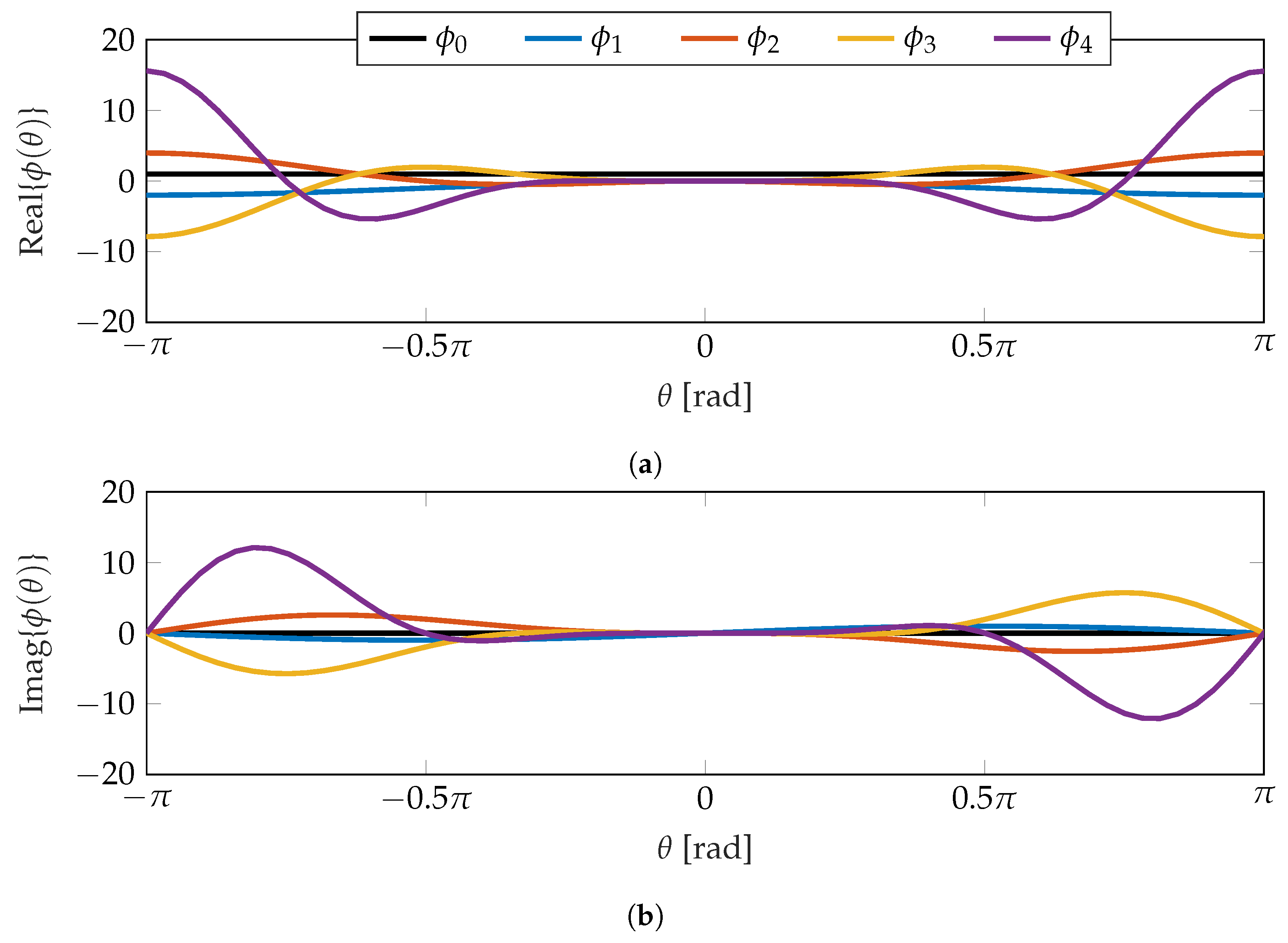
and are shown graphically in Figure 3. Because the polynomials are complex valued, the real and imaginary components are show, separately. In both cases, the polynomials are oscillatory, with the real component being symmetric about $\theta =0$, and the imaginary component being antisymmetric about $\theta =0$. Additionally, the amplitude of the oscillations increase both with increasing order and distance from $\theta =0$.

The zeroth polynomial is one, as is standard; therefore, the difference between the two generating functions given in Equations (25) and (26) will only be apparent in the calculation of moments beyond the first.

3.7. Function Complexity

As is to be expected, the computational complexity increases with increasing state dimension. It is therefore of interest to develop an expression that bounds the required number of function evaluations as a function of number of states and expansion order. Due to the many different methods of calculating inner products, all with different computational requirements, the number of functional inner products is what will be enumerated.

Let $\mathit{x}\in {\mathbb{S}}^P$ be a P-dimensional state vector consisting of angular variables, and let $\mathit{q}\in {\mathbb{N}}^P$ be the expansion order of each element in $\mathit{x}$, where $\mathbb{N}$ is the set of natural numbers, including zero. The number of inner products required to calculate the chaos coefficients in Equation (20b) for element $x_i$ is $2(q_i+1)$, where $\{i\in \mathbb{N}:k\le P\}$ and $q_i$ is the $i^{\mathrm{th}}$ element of $\mathit{q}$.

Assume that the mean, variance, and covariance are desired for/between each element. The mean does not require any extra inner products, since the mean is simply the zeroth coefficient. The variance from Equation (23) requires an additional ${(q_i+1)}^2$ inner products for a raw moment, or $q_i^2$ inner products for a central moment. Similarly, the covariance from Equation (24) between the $i^{\mathrm{th}}$ and $j^{\mathrm{th}}$ elements requires $(q_i+1)(q_j+1)$ additional evaluations for a raw moment and $q_i{q}_j$ for a central moment. Combining these into one expression, the generalized number of inner product evaluations for raw moments with $P\ge 2$ is

$$\begin{array}{c}\hfill 2(q_1+1)+{(q_1+1)}^2+\sum _{i=2}^P\left(2(q_i+1)+{(q_i+1)}^2+\sum _{j=1}^{i-1}(q_i+1)(q_j+1)\right),\end{array}$$

and for central moments is

$$\begin{array}{c}\hfill 2(q_1+1)+q_1^2+\sum _{i=2}^P\left(2(q_i+1)+q_i^2+\sum _{j=1}^{i-1}{q}_i{q}_j\right).\end{array}$$

It should be noted that this is the absolute maximum number of evaluations that is required for an entirely angular state. In many cases inner products can be precomputed, the use of orthonormal polynomials reduces the coefficient calculation inner products by two, and expansions using real valued polynomials do not require these inner product calculations at all.

4. Numerical Verification and Discussion

To test the estimation methods outlined in Section 3.5, a system with two angular degrees of freedom is considered. The correlated, nonlinear dynamics governing this body, the initial mean directions $\varphi$/$\theta$, initial USTDs, and constant angular velocities $\dot{\varphi }$/$\dot{\theta }$ are given in

Table 2. Initial conditions and governing equations of the dynamical system in Section 4.

Angle	Mean Direction	USTD	Angular Velocity (const.)	Dynamics
$\varphi$	$\pi /30$ [rad]	$0.1$ [rad]	$0.2$ [rad/s]	$\mathsf{\Delta }\varphi =\sqrt{|{\theta }_{k-1}|}\dot{\varphi }\mathsf{\Delta }T$
$\theta$	$\pi /4$ [rad]	$0.1$ [rad]	$0.2$ [rad/s]	$\mathsf{\Delta }\theta ={\theta }_{k-1}\dot{\theta }\mathsf{\Delta }T$

.

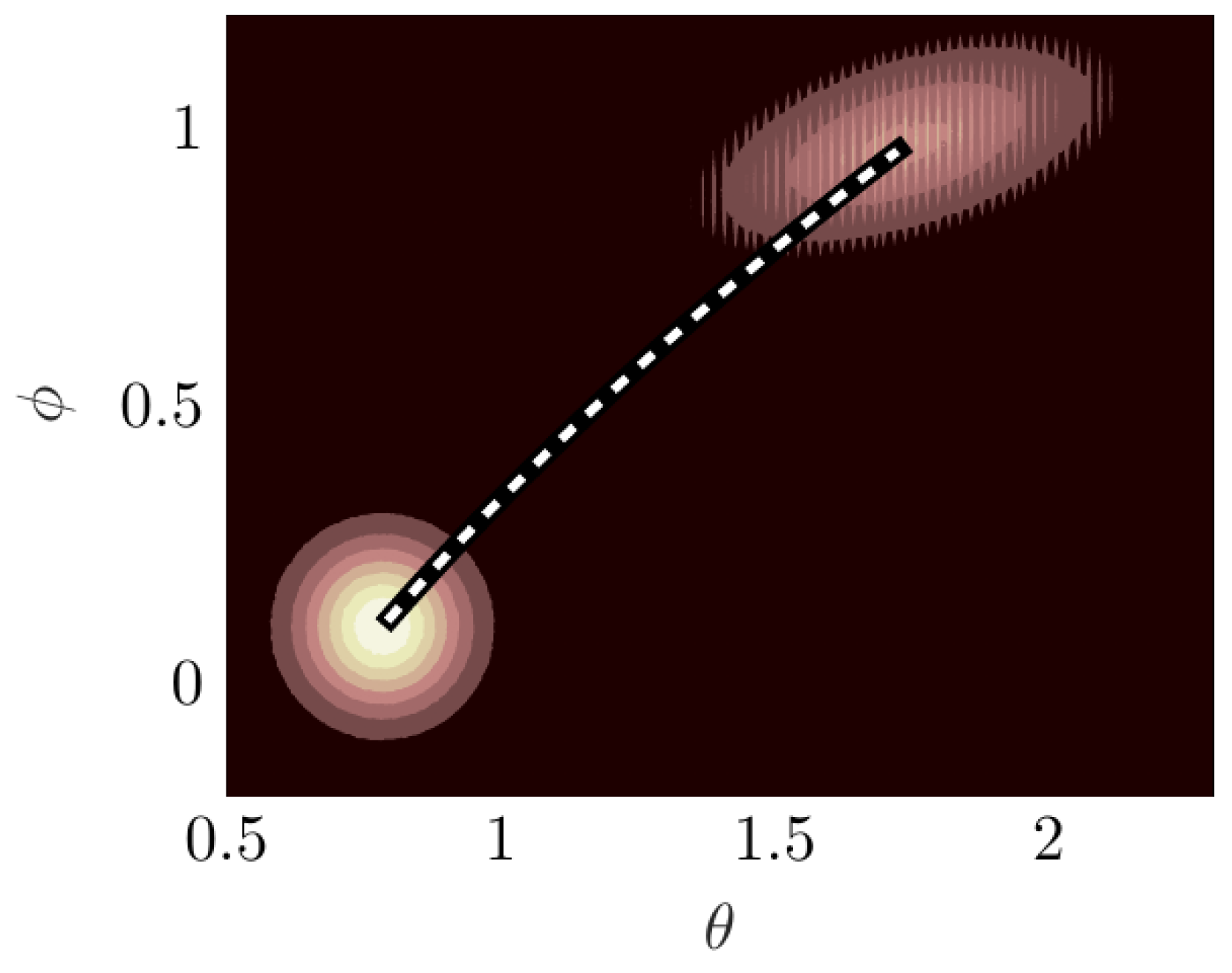
For every simulation, the run time is 4 s with $\mathsf{\Delta }T$ being $0.05$ s; this equates to 81 time steps in each simulation. In Figure 4, the joint pdf propagates from the initial conditions (bottom left) to the final state (top right). The initial joint pdf clearly reflects an uncorrelated bivariate wrapped normal distribution. After being transformed by the dynamics, the final joint pdf exhibits not just translation and scaling, but also rotation: indicating a non-zero correlation between the two angles, which is desired.

For a practical application, the mean and standard deviation/variance of each dimension, as well as the covariance between dimensions is desired. When dealing with angles, the mean direction and the standard deviation can be obtained from the first moment, omitting the second moment. Therefore, only the first moment and the covariance will be discussed. Recall the equations for the first moment and covariance are in terms of chaos coefficients and are given generally in Equations (22) and (24). Because two angles are being estimated, the supports of the integrals in Equations (22) and (24) are set as $[-\pi ,\pi )$: but it should be noted that the support is not rigidly defined this way, the only requirement is that the support length be $2\pi$.

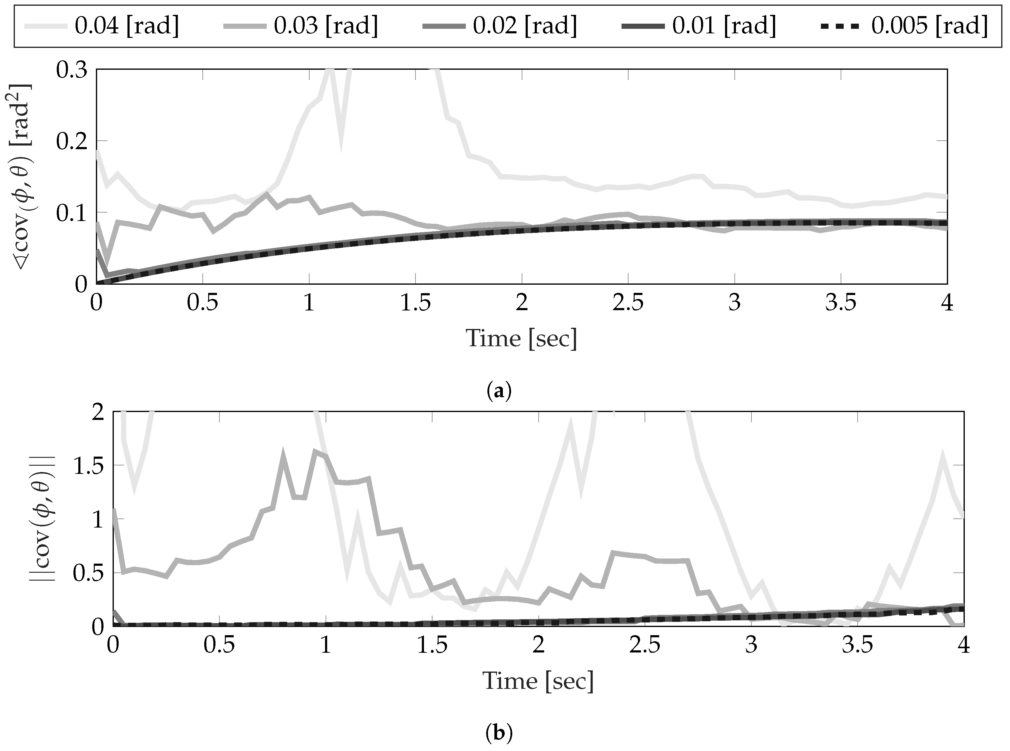
Rather than exploit the computational efficiency of methods such as quadrature integral approximations on the unit circle [50,51,52], the integrals are computed as Riemann sums. Therefore, it is necessary to determine an appropriate number of elements that provides an adequate numerical approximation, while remaining computationally feasible.

Figure 5 show the settling effect that decreasing the elemental angle has on the estimation of the covariance. Note that this figure is used to show the sensitivity of the simulation to the integration variable rather than the actual estimation of the covariance, which will be discussed later in this section. Both plots show the relative error of each estimate with respect to a Monte Carlo simulation of the joint system described in Table 2. Clearly, as the number of elements increases, the estimates begin to converge until the difference between $d\theta =0.01$ rad (629 elements) and $d\theta =0.005$ rad (1257 elements) is perceivable only near the beginning of the simulation. Because of this, it can reasonably be assumed that any error in the polynomial chaos estimate with $d\theta =0.005$ is not attributed to numerical estimation of the integrals in Equations (22) and (24). Additionally, these results should also indicate the sensitivity of the estimate to the integration variable. Even though the dynamics used in this work’s examples result in a joint pdf that somewhat resembles wrapped normal pdfs, the number of elements used in the integration must still be quite large. The final numerical element that must be covered is the Monte Carlo. For these examples, $5\times {10}^7$ samples are used in each dimension.

In each of the examples in Section 4.1, the polynomial chaos estimate first evaluates the Rogers-Szegő polynomials at each of the 1257 uniformly distributed angles ($\xi$), solves Equation (20b) for the chaos coefficients, and uses Equations (22) and (24) to estimate the mean and covariance. After this, the 1257 realizations of the state ($\mathit{\epsilon }\left(\xi \right)$) are propagated forward in time according to the system dynamics. At each time step the system is expanded using polynomial chaos to estimate the statistics.

4.1. Simulation Results

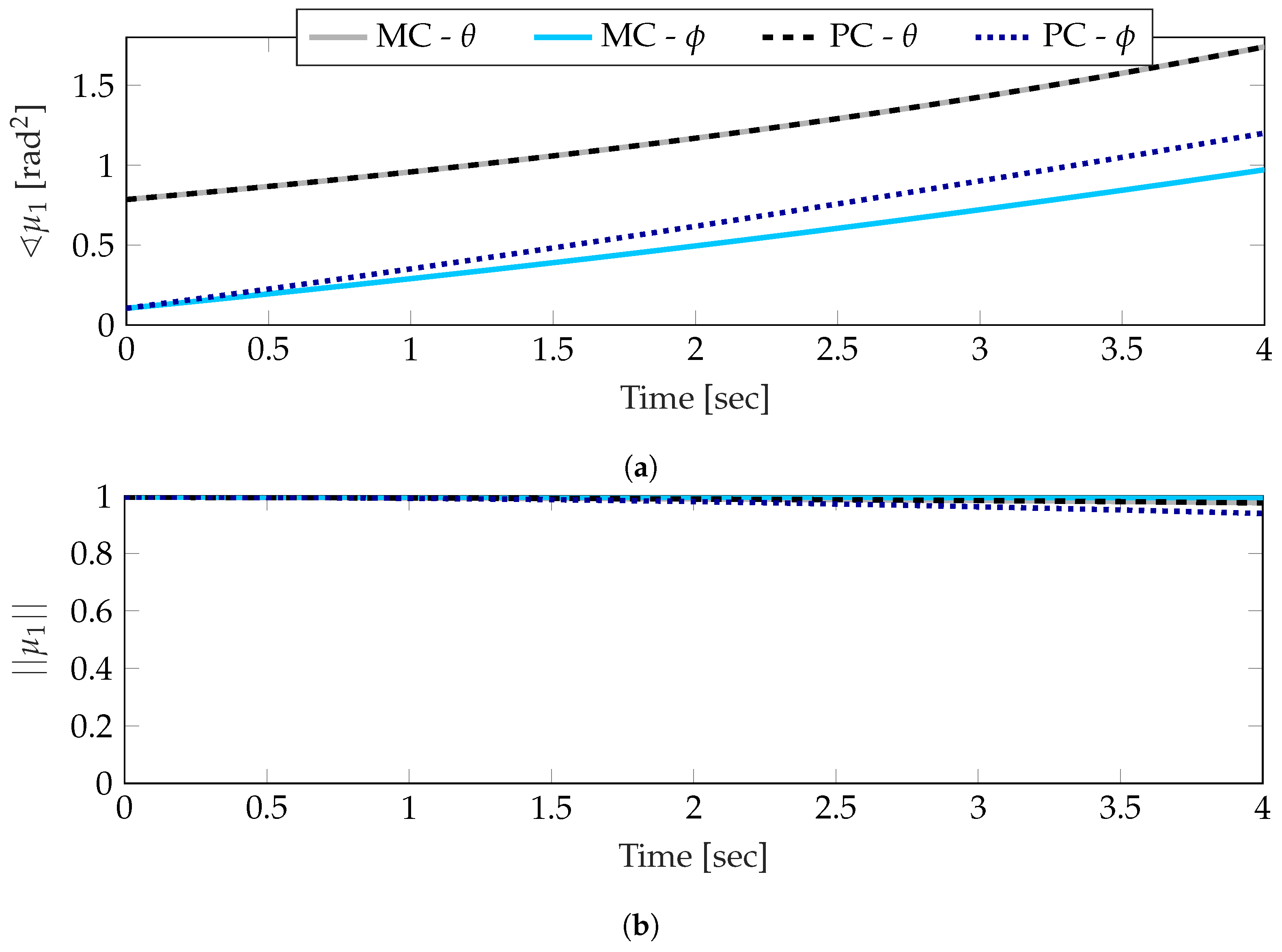
The estimations of the first moment and covariance of the system described by the simulation parameters in Table 2 are shown in Figure 6 and Figure 7. In both cases, the angle and length of the estimate are presented, rather than the exponential form used in the polynomial chaos expansion. This representation much more effectively expresses the mean and concentration components of the estimate, which are directly of interest when examining statistical moments.

Beginning with the mean estimate from a fifth order polynomial chaos expansion in Figure 6, the mean direction of the angle $\theta$ is nearly identical to the Monte Carlo estimate, while the estimate of $\varphi$ begins to drift slightly as the simulation progresses. Of the two angles, this makes the most since; recalling Table 2, only the dynamics governing $\varphi$ are correlated with $\theta$, the dynamics governing $\theta$ are only dependent on $\theta$. In comparison, the estimates of the lengths are both much closer to the Monte Carlo result. Looking closely at the end of the simulation, it can be seen that, again, $\theta$ is practically identical, and there is some small drift in $\varphi$ downwards, indicating that the estimate reflects a smaller concentration. Effectively, the estimation of the mean reflects some inaccuracy; however, this inaccuracy is partly reflected in the larger dispersion of the pdf.

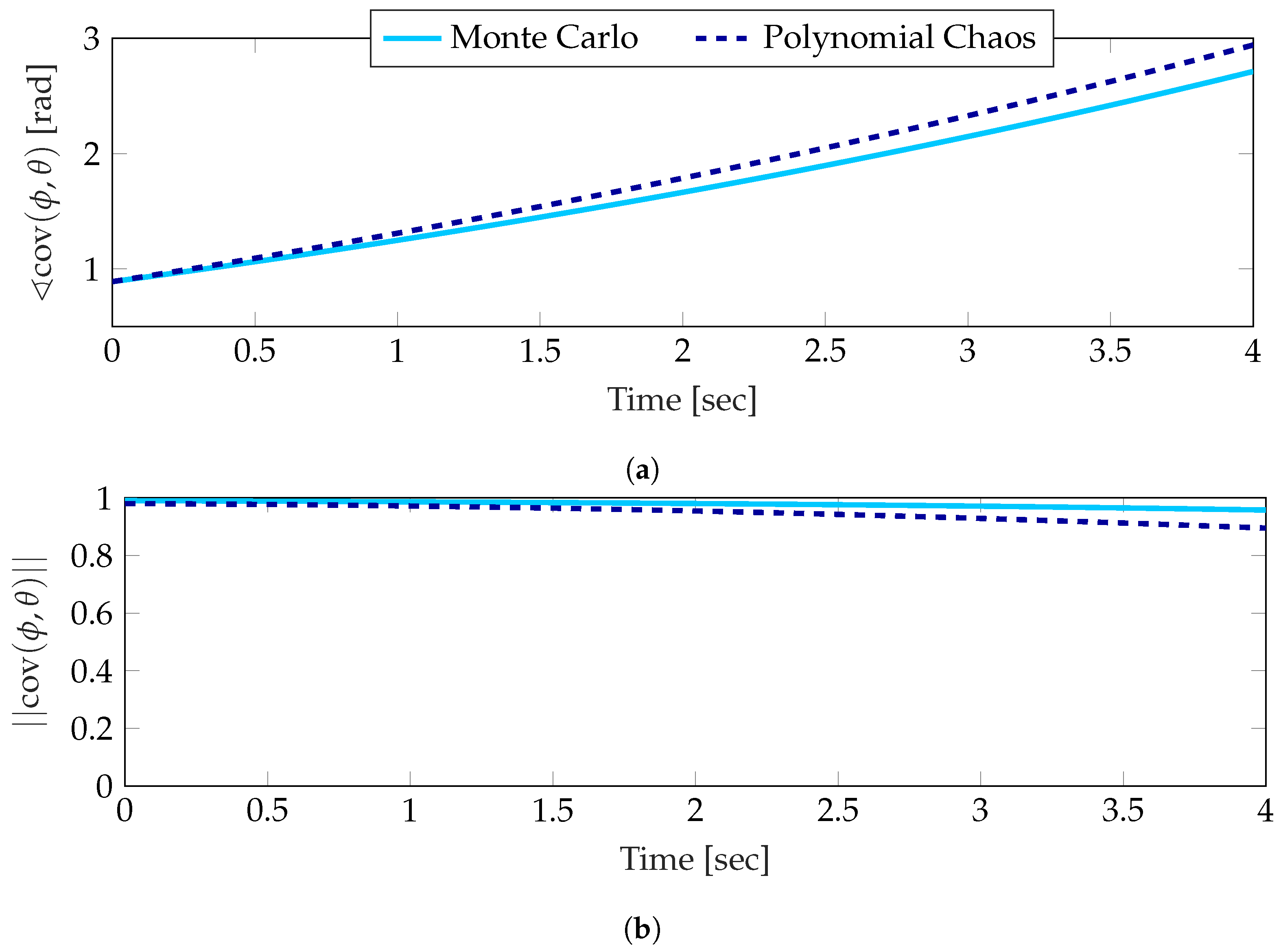
Similarly to the mean, a small drift can be seen in the estimate of the covariance in Figure 7. In both cases the initial estimate is nearly identical to the Monte Carlo result; however, throughout the simulation a small amount of drift becomes noticeable. While this drift is undesirable, the general tracking of the polynomial chaos estimate to the Monte Carlo clearly shows that the correlation between two angles can be approximated using a polynomial chaos expansion.

4.1.1. Unwrapped Standard Deviation and Joint PDF Assumptions

From the discussion of the generating function for the Rogers-Szegő polynomials Equation (25), it is clear that these polynomials are dependent on the USTD. Unfortunately this means that the polynomials are unique to any given problem, and while they can still be computed ahead of time and looked up, it is not as convenient as problems that use polynomials that are fixed (e.g., Hermite polynomials).

Additionally, the inner product in Equation (23), which describes the calculation of the covariance, requires the knowledge of the joint pdf between the two random variables. In practice, there is no reasonable way of obtaining this pdf; and if there is, then the two variables are already so well know, that costly estimation methods are irrelevant.

It is therefore of interest to investigate what effects making assumptions about the USTD and the joint pdf have on the estimates. The basis polynomials are evaluated when solving for the chaos coefficients Equation (20b) and when estimating the statistical moments Equations (22)–(25) at every time step. If no assumption is made about the USTD, then the generating function in Equation (25) or the three step recursion in Equation (5) must be evaluated at every time step as well. In either case, the computational burden can be greatly reduced if the basis polynomials remain fixed, requiring only an initial evaluation. Additionally, if the same USTD is used for both variables, than the simplification from two to one integrals in Equation (25) can be made.

While only used in the estimation of the covariance, a simplification of the joint pdf will also significantly reduce computation and increase the feasibility of the problem. The most drastic of simplifications is to use the initial, uncorrelated joint pdf. Note that the pdf used in the inner product is mean centered at zero (even for Askey chaos schemes); therefore, the validity of the estimation will not be effected by any movement of the mean.

Assuming the USTD to be fixed at $0.1$ for both random variables and the joint pdf to be stationary throughout the simulation led to estimates that are within machine precision of the unsimplified results in Figure 6 and Figure 7. This is to be expected when analyzing Askey-chaos schemes (like Hermite-chaos) that are problem invariant. In instances where the USTD of the wrapped normal distribution is low enough that probabilities at $\pm \pi$ are approximately zero, the wrapped normal distribution is effectively a segment of the unwrapped normal distribution, because the probabilities beyond $\pm \pi$ are approximately equal to zero. However, in problems where the USTD increases, the wrapped normal distribution quickly approaches a wrapped uniform distribution, this makes the time-invariant USTD a poor assumption. While a stationary USTD assumption may not hold as well for large variations in USTD, highly correlated, or poorly modeled, dynamical systems, it shows that some assumptions and simplifications can be made to ensure circular polynomial chaos is a practical method of estimation.

4.1.2. Chaos Coefficient Response

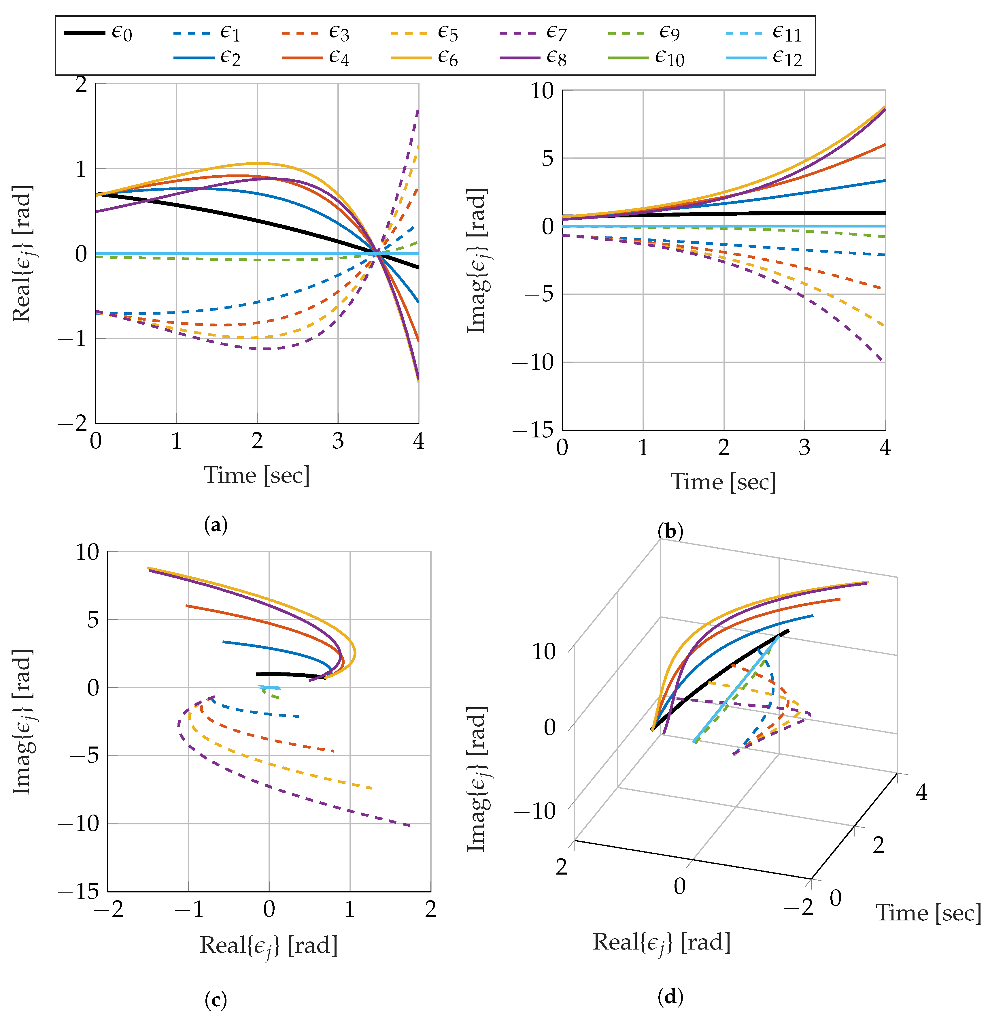
The individual chaos coefficients are not always inspected for problems using Askey-chaos simply due to the commonality of Askey-chaos. The adaptation of polynomial chaos to use the Szegő polynomials, and thus expanding from real to complex valued estimates presents a case that warrants inspection of the chaos coefficients. Figure 8 show the time evolution of the first 13 chaos coefficients (including the zeroth coefficient) that describe the random variable $\varphi$.

What becomes immediately apparent is that the coefficients are roughly anti-symmetrically paired until the length of the coefficient begins to approach zero. In this specific case, the eighth coefficient in Figure 8 initiates this trend. This is the first coefficient that does not have an initial estimate coinciding with lower ordered coefficients. All coefficients following this one show very little response to the system. This is to be expected. Recall the calculation of the chaos coefficient includes the product of polynomial and pdf as well as a division by the self inner product of each polynomial order (i.e., ${\langle {\mathrm{\Psi }}_k^2\left(\zeta \right)\rangle }_{p\left(\zeta \right)}$). The polynomial and pdf product have opposing behaviors when approaching $\pm \pi$ from 0. Whereas the polynomial oscillation amplitude increases, the tails of the pdf approach probability values of zero. This ensures the growth in the higher order polynomials is mitigated.

For brevity, only the coefficients from the variable $\varphi$ are shown. These have a much more interesting response than $\theta$ due to the nature of the dynamics. The most notable part of the coefficients from $\theta$ is that none of the coefficients ever move beyond the complex unit circle, which from Figure 8c, is clearly not the case for $\varphi$. In fact, the coefficients describing $\theta$ stay close to the complex unit circle and just move clockwise about it. Similarly, the eighth and higher coefficient lengths begin collapse to zero rad. For this problem (and presumably most problems) almost all of the information is coming from the first two coefficients. Comparing the estimates using two, three, and ten coefficients yields the same results to within machine precision. This is not surprising when considering the inner products (

Table 3. Rogers-Szegő Inner Products.

${〈{\mathit{\psi }}_{\mathit{i}},{\mathit{\psi }}_{\mathit{j}}〉}_{{\mathit{p}}_{\mathit{wn}}}$	$\mathit{j}=0$	$\mathit{j}=1$	$\mathit{j}=2$	$\mathit{j}=3$
$i=0$	1.00	−4.77e-16−3.15e-15i	−3.35e-15−2.00e-16i	−1.21e-16−1.65e-16i
$i=1$	−4.77e-16+3.15e-15i	−0.01−1.94e-16i	1.94e-4+3.06e-16i	−5.71e-06−3.27e-17i
$i=2$	−3.35e-15+2.00e-16i	1.94e-4−3.06e-16i	1.84e-4+4.61e-17i	−1.09e-05−3.70e-17i
$i=3$	−1.21e-16+1.65e-16i	−5.71e-06+3.27e-17i	−1.09e-05+3.70e-17i	−4.53e-06−2.45e-16i

) that are required to estimate the covariance; each of the inner products are effectively zero when compared with ${〈{\varphi }_0,{\varphi }_0)〉}_{p_{wn}}$ and ${〈{\varphi }_1,{\varphi }_1)〉}_{p_{wn}}$. While having to only compute two significant chaos coefficients makes computation easier, it also limits the amount of information that is used in the estimate; however, for simple problems such as this one, two significant coefficients are satisfactory.

5. Conclusions and Future Work

One method of quantifying the uncertainty of a random variable is a polynomial chaos expansion. For variables that exist only on the real line, this type of expansion has been well studied. This work developed the alterations that must be made for a polynomial chaos expansion to be valid for random variables that exist on the unit circle, specifically the complex unit circle (where the y coordinate becomes imaginary).

Previous work has shown that polynomial chaos can be used with the Rogers-Szegő polynomials to estimate the raw moments of a random variable with a wrapped normal distribution. A generalized set of expressions for the mean and covariance of multi-dimensional systems for both real and complex systems has been presented that do not make the assumption that each variable has been expanded with the same set of basis polynomials. An example of two angular random variables—one with correlated dynamics, and one without—has been presented. The mean of each random variable as well as the covariance between them is estimated and compared with Monte Carlo estimates. In the case of the uncorrelated random variable, the mean estimates are highly accurate. For the correlated random variable, the estimate is found to slowly diverge from the Monte Carlo result. A similar small divergence is observed in the covariance estimate; however, the general trend is similar enough to indicate the error is not in the formulation of the complex polynomial chaos. Additionally, an approximation to the basis polynomials and time-varying joint probability density function (pdf) is made, without loss of accuracy in the estimate. From the estimates of the mean and covariance, it is clear that the Rogers-Szegő polynomials can be used as an effective basis for angular random variable estimation. However, for more complex problems, different polynomials should be considered, specifically polynomials with an appropriate number of non-negligible self inner products.

References

- Haberberger, S.J. An IMU-Based Spacecraft Navigation Architecture Using a Robust Multi-Sensor Fault Detection Scheme. Master’s Thesis, Missouri University of Science and Technology, Rolla, MO, USA, 2016. [Google Scholar]
- Galante, J.; Eepoel, J.V.; Strube, M.; Gill, N.; Gonzalez, M.; Hyslop, A.; Patrick, B. Pose Measurement Performance of the Argon Relative Navigation Sensor Suite in Simulated-Flight Conditions. In Proceedings of the AIAA Guidance, Navigation, and Control Conference, Minneapolis, MN, USA, 13–16 August 2012. [Google Scholar]
- Latella, C.; Lorenzini, M.; Lazzaroni, M.; Romano, F.; Traversaro, S.; Akhras, M.A.; Pucci, D.; Nori, F. Towards Real-Time Whole-Body Human Dynamics Estimation Through Probabilistic Sensor Fusion Algorithms. Auton. Robot. 2019, 43, 1591–1603. [Google Scholar] [CrossRef] [Green Version]
- Lubey, D.P.; Scheeres, D.J. Supplementing state and dynamics estimation with information from optimal control policies. In Proceedings of the 17th International Conference on Information Fusion (FUSION), Salamanca, Spain, 7–10 July 2014; pp. 1–7. [Google Scholar]
- Imani, M.; Ghoreishi, S.F.; Braga-Neto, U.M. Bayesian Control of Large MDPs with Unknown Dynamics in Data-Poor Environments. In Advances in Neural Information Processing Systems 31; Curran Associates, Inc.: Red Hook, NY, USA, 2018; pp. 8146–8156. [Google Scholar]
- Hughes, D.L. Comparison of Three Thrust Calculation Methods Using In-Flight Thrust Data; NASA TM-81360; NASA: Washington, DC, USA, 1981; Unpublished. [Google Scholar]
- Julier, S.; Uhlmann, J.; Durrant-Whyte, H.F. A New Method for the Nonlinear Transformation of Means and Covariances in Filters and Estimators. IEEE Trans. Autom. Control 2000, 45, 477–482. [Google Scholar] [CrossRef] [Green Version]
- Wu, C.C.; Bossaerts, P.; Knutson, B. The Affective Impact of Financial Skewness on Neural Activity and Choice. PLoS ONE 2011, 6, e16838. [Google Scholar] [CrossRef] [PubMed] [Green Version]
- Anderson, T.; Mattson, C. Propagating Skewness and Kurtosis Through Engineering Models for Low-Cost, Meaningful, Nondeterministic Design. J. Mech. Des. 2012, 134, 100911. [Google Scholar] [CrossRef] [Green Version]
- Wiener, N. The Homogeneous Chaos. Am. J. Math. 1938, 60, 897–936. [Google Scholar] [CrossRef]
- Janson, S. Gaussian Hilbert Spaces; Cambridge Tracts in Mathematics; Cambridge University Press: New York, NY, USA, 1997; Chapter 1.2. [Google Scholar]
- Alexanderian, A. Gaussian Hilbert Spaces and Homogeneous Chaos: From theory to applications. 2013; Unpublished. [Google Scholar]
- Eldred, M. Recent Advances in Non-Intrusive Polynomial Chaos and Stochastic Collocation Methods for Uncertainty Analysis and Design. In Proceedings of the 50th AIAA/ASME/ASCE/AHS/ASC Structures, Structural Dynamics, and Materials Conference, Palm Springs, CA, USA, 4–7 May 2009; Volume 4, pp. 2078–2114. [Google Scholar]
- Ng, L.; Eldred, M. Multifidelity Uncertainty Quantification Using Non-Intrusive Polynomial Chaos and Stochastic Collocation. In Proceedings of the 53rd AIAA/ASME/ASCE/AHS/ASC Structures, Structural Dynamics and Materials Conference, Honolulu, HI, USA, 23–26 April 2012; Volume 9, pp. 7669–7685. [Google Scholar]
- Savin, E.; Faverjon, B. Higher-Order Moments of Generalized Polynomial Chaos Expansions for Intrusive and Non-Intrusive Uncertainty Quantification. In Proceedings of the 19th AIAA Non-Deterministic Approaches Conference, Grapevine, TX, USA, 9–13 January 2017; pp. 215–223. [Google Scholar]
- Xiu, D.; Karniadakis, G.E. The Wiener-Askey Polynomial Chaos for Stochastic Differential Equations. SIAM J. Sci. Comput. 2003, 24, 619–644. [Google Scholar] [CrossRef]
- Schmid, C.L.; DeMars, K.J. Minimum Divergence Filtering Using a Polynomial Chaos Expansion. In Proceedings of the AAS/AIAA Astrodynamics Specialist Conference, Stevenson, WA, USA, 20–24 August 2017. [Google Scholar]
- Xiu, D.; Karniadakis, G.E. Modeling Uncertainty in Flow Simulations via Generalized Polynomial Chaos. J. Comput. Phys. 2003, 187, 137–167. [Google Scholar] [CrossRef]
- Hosder, S.; Walters, R.W.; Perez, R. A Non-Intrusive Polynomial Chaos Method for Uncertainty Propagation in CFD Simulations. In Proceedings of the 44th AIAA Aerospace Sciences Meeting and Exhibit, Reno, NV, USA, 9–12 January 2006. [Google Scholar]
- Hosder, S.; Walters, R.W.; Balch, M. Point-Collocation Non-Intrusive Polynomial Chaos Method for Stochastic Computational Fluid Dynamics. AIAA J. 2010, 48, 2721–2730. [Google Scholar] [CrossRef]
- Hosder, S.; Walters, R.W. Non-Intrusive Polynomial Chaos Methods for Uncertainty Quantification in Fluid Dynamics. In Proceedings of the 48th AIAA Aerospace Sciences Meeting, Orlando, FL, USA, 4–7 January 2010; pp. 1580–1595. [Google Scholar]
- Jones, B.A.; Doostan, A.; Born, G.H. Nonlinear Propagation of Orbit Uncertainty Using Non-Intrusive Polynomial Chaos. J. Guid. Control. Dyn. 2013, 36, 430–444. [Google Scholar] [CrossRef] [Green Version]
- Vittaldev, V.; Russell, R.P.; Linares, R. Spacecraft Uncertainty Propagation Using Gaussian Mixture Models and Polynomial Chaos Expansions. J. Guid. Control. Dyn. 2016, 39, 2615–2626. [Google Scholar] [CrossRef] [Green Version]
- Mardia, K.; Jupp, P. Directional Statistics; Wiley Series in Probability and Statistics; John Wiley & Sons, Inc.: Hoboken, NJ, USA, 2009. [Google Scholar]
- Markley, F.L. Attitude Error Representations for Kalman Filtering. J. Guid. Control. Dyn. 2003, 26, 311–317. [Google Scholar] [CrossRef]
- Darling, J.E. Bayesian Inference for Dynamic Pose Estimation Using Directional Statistics. Ph.D. Thesis, Missouri University of Science and Technology, Rolla, MO, USA, 2016. [Google Scholar]
- Schmid, C.L.; DeMars, K.J. Polynomial Chaos Confined to the Unit Circle. In Proceedings of the AAS/AIAA Astrodynamics Specialist Conference, Snowbird, UT, USA, 19–23 August 2018; pp. 2239–2256. [Google Scholar]
- Jones, B.A.; Balducci, M. Uncertainty Propagation of Equinoctial Elements Via Stochastic Expansions. In Proceedings of the John L. Junkins Dynamical Systems Symposium, College Station, TX, USA, 20–21 May 2018. [Google Scholar]
- Andrews, G.E.; Askey, R. Classical Orthogonal Polynomials. Polynômes Orthogonaux et Applications; Brezinski, C., Draux, A., Magnus, A.P., Maroni, P., Ronveaux, A., Eds.; Springer: Berlin/Heidelberg, Germany, 1985; pp. 36–62. [Google Scholar]
- Askey, R.; Wilson, J. Some Basic Hypergeometric Orthogonal Polynomials that Generalize Jacobi Polynomials; Number 319 in American Mathematical Society: Memoirs of the American Mathematical Society; American Mathematical Society: Providence, RI, USA, 1985; Chapter 1. [Google Scholar]
- Koekoek, R.; Lesky, P.A.; Swarttouw, R.F. Hypergeometric Orthogonal Polynomials and Their q-Analogues; Springer Monographs in Mathematics; Springer: Berlin/Heidelberg, Germany, 2010. [Google Scholar]
- Szegő, G. Orthogonal Polynomials; American Mathematical Society Colloquium Publications, American Mathematical Society: Providence, RI, USA, 1959; Volume 23, Chapter 11; pp. 287–295. [Google Scholar]
- Simon, B. Orthogonal Polynomials on the Unit Circle (Colloquium Publications); American Mathematical Society: Providence, RI, USA, 2005; Volume 54. [Google Scholar]
- Simon, B. Orthogonal Polynomials on the Unit Circle: New Results. arXiv 2004, arXiv:math.SP/math/0405111. [Google Scholar]
- Geronimus, Y.L. Orthogonal Polynomials: Estimates, Asymptotic Formulas, and Series of Polynomials Orthogonal on the Unit Circle and on an Interval. Math. Gaz. 1962, 46, 354–355. [Google Scholar] [CrossRef]
- Ismail, M.E.; Ruedemann, R.W. Relation Between Polynomials Orthogonal on the Unit Circle with Respect to Different Weights. J. Approx. Theory 1992, 71, 39–60. [Google Scholar] [CrossRef] [Green Version]
- Jagels, C.; Reichel, L. On the Construction of Szegő Polynomials. J. Comput. Appl. Math. 1993, 46, 241–254. [Google Scholar] [CrossRef] [Green Version]
- Jones, W.B.; Njåstad, O.; Thron, W.J. Moment Theory, Orthogonal Polynomials, Quadrature, and Continued Fractions Associated with the Unit Circle. Bull. Lond. Math. Soc. 1989, 21, 113–152. [Google Scholar] [CrossRef]
- Atakishiyev, N.M.; Nagiyev, S.M. On the Rogers-Szegő Polynomials. J. Phys. Math. Gen. 1994, 27, L611. [Google Scholar] [CrossRef]
- Hou, Q.; Lascoux, A.; Mu, Y. Continued Fractions for Rogers-Szegő Polynomials. Numer. Algorithms 2004, 35, 81–90. [Google Scholar] [CrossRef]
- Vinroot, C.R. Multivariate Rogers-Szegő Polynomials and Flags in Finite Vector Spaces. arXiv 2010, arXiv:math.CO/1011.0984. [Google Scholar]
- Szabłowski, P.J. On q-Hermite Polynomials and Their Relationship With Some Other Families of Orthogonal Polynomials. Demonstr. Math. 2011, 46, 679–708. [Google Scholar] [CrossRef]
- Andrews, G. The Theory of Partitions; Cambridge Mathematical Library, Cambridge University Press: Cambridge, UK, 1998. [Google Scholar]
- Fisher, R. Dispersion on a Sphere. Proc. R. Soc. London. Ser. Math. Phys. Eng. Sci. 1953, 217, 295–305. [Google Scholar] [CrossRef]
- Watson, G.S.; Williams, E.J. On the Construction of Significance Tests on the Circle and the Sphere. Biometrika 1956, 43, 344–352. [Google Scholar] [CrossRef]
- Mardia, K.V. Distribution Theory for the von Mises-Fisher Distribution and Its Application. In A Modern Course on Statistical Distributions in Scientific Work; Patil, G.P., Kotz, S., Ord, J.K., Eds.; Springer: Dordrecht, The Netherlands, 1975; pp. 113–130. [Google Scholar]
- Bogachev, V. Gaussian Measures; Mathematical Surveys and Monographs, American Mathematical Society: Providence, RI, USA, 2015. [Google Scholar]
- Cameron, R.H.; Martin, W.T. The Orthogonal Development of Non-Linear Functionals in Series of Fourier-Hermite Functionals. Ann. Math. 1947, 48, 385–392. [Google Scholar] [CrossRef]
- Fubini, G. Sugli Integrali Multipli: Nota; Reale Accademia dei Lincei: Rome, Italy, 1907. [Google Scholar]
- Cruz-Barroso, R.; Mendoza, C.D.; Perdomo-Pío, F. Szegő-Type Quadrature Formulas. J. Math. Anal. Appl. 2017, 455, 592–605. [Google Scholar] [CrossRef]
- Bultheel, A.; González-Vera, P.; Hendriksen, E.; Njåstad, O. Orthogonal Rational Functions and Quadrature on the Unit Circle. Numer. Algorithms 1992, 3, 105–116. [Google Scholar] [CrossRef] [Green Version]
- Daruis, L.; González-Vera, P. Szegő Polynomials and Quadrature Formulas on the Unit Circle. Appl. Numer. Math. 2001, 36, 79–112. [Google Scholar] [CrossRef]
Figure 1.
Common Circular probability density functions (pdfs). (a) Circular von Mises distribution for multiple values of . (b) Wrapped normal distribution for multiple values of .
Figure 2.
Error induced by approximating a circular distribution as linear, tangent at the mean. (a) Wrapped normal distribution with pdf . (b) Wrapped normal distribution approaching wrapped uniform distribution with pdf . (c) Projection of onto a plane tangent to the unit circle. (d) Projection of onto a plane tangent to the unit circle. (e) Error associated with projecting onto a plane tangent to the unit circle. (f) Error associated with projecting onto a plane tangent to the unit circle.
Figure 3.
The zeroth through fourth Rogers-Szegő polynomials with an unwrapped standard deviation of 0.1. (a) Real Component. (b) Imaginary Component.
Figure 4.
Evolution of the joint pdf from uncorrelated to correlated bivarite wrapped normal pdf.
Figure 5.
Effects of integration variable on estimated covariance relative error. Each line represents a different elemental angle ranging from to rad. (a) Angle Component. (b) Length Component.
Figure 6.
Estimation of the first moment of both angles using a fifth order polynomial chaos expansion compared against Monte Carlo simulation. (a) Angle Component. (b) Length Component.
Figure 7.
Estimation of the covariance between the two angles using a fifth order polynomial chaos expansion compared against Monte Carlo simulation. (a) Angle Component. (b) Length Component.
Figure 8.
Time evolution of the first 13 chaos coefficients describing the random variable . (a) Real Coefficient Evolution. (b) Imaginary Coefficient Evolution. (c) Imaginary and Real Coefficient Evolution. (d) Complex Coefficient Evolution.