Bivariate Thiele-Like Rational Interpolation Continued Fractions with Parameters Based on Virtual Points

Abstract

The interpolation of Thiele-type continued fractions is thought of as the traditional rational interpolation and plays a significant role in numerical analysis and image interpolation. Different to the classical method, a novel type of bivariate Thiele-like rational interpolation continued fractions with parameters is proposed to efficiently address the interpolation problem. Firstly, the multiplicity of the points is adjusted strategically. Secondly, bivariate Thiele-like rational interpolation continued fractions with parameters is developed. We also discuss the interpolant algorithm, theorem, and dual interpolation of the proposed interpolation method. Many interpolation functions can be gained through adjusting the parameter, which is flexible and convenient. We also demonstrate that the novel interpolation function can deal with the interpolation problems that inverse differences do not exist or that there are unattainable points appearing in classical Thiele-type continued fractions interpolation. Through the selection of proper parameters, the value of the interpolation function can be changed at any point in the interpolant region under unaltered interpolant data. Numerical examples are given to show that the developed methods achieve state-of-the-art performance.

1. Introduction

The interpolation method plays a critical role in approximation theory and is a classical topic in numerical analysis [1,2,3,4,5,6]. It is believed that interpolation polynomial and rational interpolation are two popular interpolation methods. They have many applications, such as image interpolation processing, numerical approximation [1], extensive applications in terms of arc structuring [1,2], and so on. Kuchminska et al. [3] proposed a Newton-Thiele-like Interpolating formula for two variate interpolation. Pahirya et al. [4] developed the problem of the interpolant function of bivariate by two-dimensional continued fractions. Li et al. [5] generalized Thiele’s expansion of a univariate rational interpolation function to the Thiele-Newton blending rational interpolation. The authors also developed the Viscovatov-like algorithm to calculate the coefficients of Thiele-Newton’s expansion. Cuyt et al. [6] used a multivariate data fitting technique to solve various scientific computing problems in filtering, meta-modelling, queueing, computational finance, networks, graphics, and more. Li et al. [7] analyzed the fractional-order unified chaotic system by different fractional calculus numerical methods. Xu et al. [8] introduced the truncated exponential radial function for surface modeling. Massopust [9] constructed non-stationary fractal functions and interpolation based on non-stationary versions of fixed points. In recent years, different aspects of rational multivariate interpolation were studied, especially in Newton form. Cuyt et al. [10] define multivariate divided differences of the multivariate Newton–Padé approximants. Akal et al. [11] modified Cuyt and Verdonk’s approach to multivariate Newton–Padé approximations. Ravi [12] studied the minimal rational interpolation problem using algebrogeometric methods. Bertrand et al. [13] proposed a new polynomial projector on a space of functions of many variables, and studied the main approximation properties of the new projectors. One multipoint multivariate polynomial interpolation method from the Goodman–Hakopian polynomial interpolation was generalized to the case of rational interpolation in the paper [14]. The authors presented the scale of mean value multipoint multivariate Padé interpolations which includes as particular cases both the scale of mean value polynomial interpolations and the multipoint multivariate Padé approximations. Based on the collocation polynomial and Hermite interpolation, Li et al. [15] proposed a numerical explicit gradient scheme, which has higher convergence order.

The interpolation method also was applied to graphic image morphing and image processing [16,17,18,19,20,21,22,23,24]. In the paper [16], an effective directional Bayer color filter array demosaicking method based on residual interpolation is presented. The proposed algorithm guaranteed the quality of color images and reduced the computational complexity. Zhou et al. [17] developed an interpolation filter called an all-phase discrete sine transform filter and used it for image demosaicking. Min et al. [18] proposed a nonlinear approximation method based on Taylor series to describe and approximate images with intensity inhomogeneity. He et al. [19,20] presented a Thiele-Newton’s rational interpolation function in the polar coordinates which was then applied to image super-resolution. The new method had a lower time cost and a better magnified effect. Yao et al. [21] proposed a new approach to bivariate rational interpolation. The presented interpolation method was identified by the values of shape parameters and scaling factors from the paper [21]. Zhang et al. [22] presented a single-image super-resolution algorithm based on rational fractal interpolation. Based on a multi-scale optical flow reconstruction scheme, Ahn et al. [23] proposed a fast 4K video frame interpolation method. Wei et al. [24] adopted the bilinear interpolation to obtain the Region of Interest pooling layer in image manipulation detection. In recent years, Zhang et al. [25,26] have reported on some new types of weighted blending spline interpolation. By selecting different coefficients and appropriate parameters, the value of the spline interpolation function can be modified at any point, in the interpolant region under unchanging interpolant data, so the interpolation functions of geometric surfaces can be adjusted, even for the given data, in actual design, but the computation is complicated. One of the authors proposed an associated continued fractions rational interpolation and its Viscovatov algorithm through Taylor expansion, proposed some different types of bivariate interpolation, and studied several general interpolation functions [27]. Tang and Zou [28,29] studied and provided some general interpolation frames with many interpolation formulae. For the given interpolation data, it could handle some special interpolant problems through selecting parameters appropriately. However, it is still a quite difficult problem to select appropriate parameters and then design the interpolation format while meeting the conditions in the computational process. It is difficult to determine such a function without the process of comparison and trial. Zhao et al. [30] presented the block-based Thiele-like blending rational interpolation. For the given interpolation points, many types of block-based Thiele-like blending rational interpolation were studied based on different block points of data. For image processing and computer-aided geometric design, there is still substantial demand for complicated models and the integration of design and fabrication, but two problems remain:

• How to construct a proper polynomial or rational interpolation with explicit mathematical expression and a simple calculation which make the function easy to use and convenient to study theoretically;
• For the given data, how to modify the curve or surface shape to enable the function to meet the actual requirements.

In the classical interpolation method, the interpolation function is unique to the interpolation points, and it is almost impossible to resolve the above two problems.

Thus, this raises an interesting question: whether many unique rational interpolations based on inverse difference exist. At present, the Thiele-type rational interpolation continued fractions is the hot topic regarding methods of rational interpolation; however, it is unique for the given interpolation data, and this limits its application. The Thiele-like rational interpolation continued fractions may meet nonexistent inverse differences and unattainable points. To avoid the problems mentioned above, this paper aims to develop bivariate Thiele-like rational interpolation continued fractions by introducing one or more parameters, which can adjust the shape of the curves or surfaces without altering the given interpolation points, so as to meet the practical requirements. Meanwhile, in contrast to the classical interpolation method in [1], our method can avoid unattainable points and nonexistent inverse differences in interpolation problems and performs better. In contrast to the interpolation methods presented in [1,28,31,32], it is unnecessary to adjust the nodes, and only the addition of multiple numbers in the sight of unattainable points is required, which makes it simple to numerate. To solve the above problem, in the paper [33,34,35], the authors developed a univariate Thiele-like rational interpolation continued fractions with parameters. The question can be solved with the proposed method in the paper, but the authors only discussed the univariate case. We generalize the results to the bivariate case in this paper.

The organization of the paper is as follows: We give a brief review on univariate Thiele-like rational interpolation continued fractions with parameters and discuss a special rational interpolation problem where unattainable points and inverse differences do not exist, and solve it through univariate Thiele-like rational interpolation with parameters in Section 2. We propose four bivariate Thiele-like branched rational interpolation continued fractions with parameters in Section 3. In addition to the bivariate Thiele-like branched rational interpolation continued fractions with unattainable points, the dual interpolation format of bivariate Thiele-like branched rational interpolation continued fractions with a single parameter and bivariate Thiele-like branched rational interpolation continued fractions with a nonexistent partial inverse difference are also discussed. As an application of the proposed methods, numerical examples are given to illustrate the effectiveness of the methods in Section 4.

2. Univariate Thiele-Like Interpolation Continued Fractions with Parameters

Let us consider the following univariate rational interpolation problem. If we consider a function $y=f(x)$ and support points set {(x₀,y₀),(x₁,y₁),…(x_n,y_n)} on interval $\left[a,b\right]$, we can gain the following classical Thiele-like rational interpolation continued fractions [1]:

$$R_n(x)=b_0+\frac{x-x_0^{}}{b_1}\begin{array}{c}\\ +\end{array}\frac{x-x_1}{b_2}\begin{array}{c}\\ +\cdots +\end{array}\frac{x-x_{n-1}}{b_n^{}}$$

(1)

where $b_i(i=1,\dots ,n)$ represents the inverse differences of $f(x)$.

2.1. Thiele-Like Rational Interpolation Continued Fractions with Parameter

It is well known from the literature that if Thiele-type continued fractions rational interpolation functions exist, they are unique compared with the popular method. This is inconvenient for practical application. To solve this problem, many scholars have proposed several improved methods. Zhao et al. [25] demonstrated the block-based Thiele-like blending rational interpolation. For a given set of interpolation points, many kinds of Thiele-type continued fractions interpolation functions can be constructed based on different block points. However, since every interpolation function is constructed for a special block method, one cannot derive different interpolation functions for special block points, and the interpolation function cannot adjust and may meet unattainable points. For a special block-based method, one must construct a polynomial or rational interpolation and calculate the block-based inverse difference and then construct the block-based Thiele-like blending rational interpolation. This requires a large amount of calculation and is inconvenient for the interpolation application. So, Zou et al. [33,34,35] constructed several novel univariate Thiele-like rational interpolation continued fractions with parameters, which has many advantages. By introducing a new parameter, $\lambda$ ($\lambda \ne 0$), the authors [33,34] considered taking a point of the original points $(x_k,y_k)(k=0,1,\dots ,n)$ as a virtual double point, and the multiplicity of the other points remains the same.

Let

$$y_i^0=y_i,i=0,1,\dots ,n.$$

(2)

Suppose $k<n$, when $j=1,\dots ,k+1$, for $i=j,j+1,\dots ,n$,

$$y_i^j=\frac{x_i-x_{j-1}}{y_i^{j-1}-y_{j-1}^{j-1}}.$$

(3)

For $i=k+1,k+2,\dots ,n$,

$$z_i^{k+1}=\frac{x_i-x_k}{y_i^{k+1}-\frac{1}{\lambda }}.$$

(4)

When $j=k+2,k+3,\dots ,n$, for $i=j,j+1,\dots ,n$,

$$z_i^j=\frac{x_i-x_{j-1}}{z_i^{j-1}-z_{j-1}^{j-1}}.$$

(5)

The Thiele-like rational interpolation continued fractions with a single parameter have the formula as follows:

$$R_n{}^{(0)}(x)=c_0+\frac{x-x_0^{}}{c_1}\begin{array}{c}\\ +\cdots +\end{array}\frac{x-x_{k-1}}{c_k}\begin{array}{c}\\ +\end{array}\frac{x-x_k}{c_{k+1}^0}\begin{array}{c}\\ +\end{array}\frac{x-x_k}{c_{k+1}^{}}\begin{array}{c}\\ +\end{array}\frac{x-x_{k+1}}{c_{k+2}^{}}\begin{array}{c}\\ +\cdots +\end{array}\frac{x-x_{n-1}}{c_n^{}},$$

(6)

where

$$\begin{gathered} c_i=\{\begin{array}{l}{y}_i^i,i=0,1,\dots ,k,\\ z_i^i,i=k+1,k+2,\dots ,n,\end{array} \\ {c}_{k+1}^0=\frac{1}{\lambda }. \end{gathered}$$

(7)

Without loss of generality, the authors [33,34] generalized the results to the Thiele-like rational interpolation continued fractions with two parameters. The authors discussed two categories: an arbitrary point of the original points is considered as a treble virtual point; two arbitrary points of original points are considered as the virtual double points. It can be seen that the new kind of Thiele-like continued fraction is not unique, and it satisfies the given interpolation condition. We know that it could meet nonexistent inverse differences and unattainable points in the classical Thiele-type continued fractions interpolation. As a fact, the Thiele-like rational interpolation continued fractions with parameters can solve the above interpolation problem. We discuss this problem in the next two subsections.

2.2. The Interpolation Problem with Unattainable Points

Definition 1

([31]). Suppose the given point is $D=\{(x_i,y_i)|i=0,1,\dots ,n\}$ and $x_i$ is diverse, $R(x)=\frac{N(x)}{D(x)}$ is the Thiele-type interpolation continued fractions in Formula (1) if $(x_k,y_k)$ satisfies

$$N(x_k)-D(x_k)y_k=0,R(x_k)=\frac{N(x_k)}{D(x_k)}\ne y_k.$$

(8)

Then, $(x_k,y_k)$ is an unattainable point of $R(x)$.

Theorem 1

([31,32]). Suppose the given point is $D=\{(x_i,y_i)|i=0,1,\dots ,n\}$, and $x_i$ is diverse, the Thiele-type interpolation continued fraction is as shown in Formula (1), where $b_k\ne \infty$, $(k=0,1,\dots ,n-1)$, $b_n\ne 0$, and then the necessary and sufficient condition of $(x_k,y_k)$ for an unattainable point is

$$R_k(x_k)=0,$$

(9)

where $R_k(x)$ = $\frac{N_k(x)}{D_k(x)}$ is irreducible and

$$R_{n-1}(x)=b_n,R_i(x)=b_{i+1}+(x-x_{i+1})R_{{}_{i+1}}{}^{-1}(x),i=n-2,n-3,\dots ,k.$$

(10)

Theorem 2.

The Thiele-like rational interpolation continued fractions with a single parameter defined by Equations (2)–(5) satisfies

$$R_n{}^{(0)}(x_k)=y_k.$$

(11)

Proof. 

From Equation (6), let $R_k{}^{(0)}(x)=\frac{1}{\lambda }+\frac{x-x_k}{R_{k+1}{}^{(0)}(x)}$, where

$$\begin{gathered} R_n{}^{(0)}(x)=c_n, \\ {R}_i{}^{(0)}(x)=c_i+\frac{x-x_i}{R_{i+1}{}^{(0)}(x)}(i=n-1,n-2,\dots ,k+1). \end{gathered}$$

Then, $R_k{}^{(0)}(x_k)=\frac{1}{\lambda }\ne 0$ from Theorem 1, $(x_k,y_k)$ is an unattainable point of $R_n{}^{(0)}(x)$, and then we have $R_n{}^{(0)}(x_k)=y_k$.

The proof is complete. □

2.3. The Thiele-Like Rational Interpolation Continued Fractions Problem with a Nonexistent Inverse Difference

Given diverse interpolation data $\{(x_0,y_0),(x_1,y_1),$$\dots ,$ $(x_n,y_n)\}$, in the process of constructing Thiele-like rational interpolation continued fractions, the inverse difference would be $\infty$ if the denominator equals zero, i.e., the inverse difference does not exist, which results in the failure of Thiele-type continued fractions interpolation function. Considering this case, assume that $y_{k+1}^{k+1}$ does not exist (i.e., $y_{k+1}^{k+1}=\infty$), we introduce a parameter $\eta (\eta \ne 0)$, and construct the novel inverse difference as shown in

Table 1. Inverse differences table where an inverse difference does not exist.

Nodes	0 Order Inverse Differences	1 Order Inverse Differences		$\mathit{k}$	$\mathit{k}+1\mathbf{Order}\mathbf{Inverse}\mathbf{Differences}$	$\mathit{k}+2\mathbf{Order}\mathbf{Inverse}\mathbf{Differences}$		$\mathit{n}+1\mathbf{Order}\mathbf{Inverse}\mathbf{Differences}$
$x_0$	$y_0^0$
$x_1$	$y_1^0$	$y_1^1$
$\begin{array}{c}⋮\end{array}$	$\begin{array}{c}⋮\end{array}$	$\begin{array}{c}⋮\end{array}$	$\ddots$
$x_k$	$y_k^0$	$y_k^1$	$\cdots$	$y_k^k$
$x_k$	$y_k^0$	$y_k^1$	$\cdots$	$y_k^k$	$\frac{1}{\eta }$
$x_{k+1}$	$y_{k+1}^0$	$y_{k+1}^1$	$\cdots$	$y_{k+1}^k$	$y_{k+1}^{k+1}$	$z_{k+1}^{k+1}$
$\begin{array}{c}⋮\end{array}$	$\begin{array}{c}⋮\end{array}$	$\begin{array}{c}⋮\end{array}$	$\cdots$	$⋮$	$⋮$	$⋮$	$\ddots$
$x_n$	$y_n^0$	$y_n^1$	$\cdots$	$\begin{array}{c}{y}_n^k\end{array}$	$y_n^{k+1}$	$z_n^{k+1}$	$\cdots$	$z_n^n$

.

From Equation (4), we can get

$$z_{k+1}^{k+1}=\frac{x_{k+1}-x_k}{y_{k+1}^{k+1}-\frac{1}{\eta }}=\frac{x_{k+1}-x_k}{\infty -\frac{1}{\eta }}=0.$$

(12)

Using the method given in Formula (6), we can construct a Thiele-like rational interpolation continued fractions with a parameter:

$$R_n{}^{(3)}(x)=c_0+\frac{x-x_0^{}}{c_1}\begin{array}{c}\\ +\cdots +\end{array}\frac{x-x_{k-1}}{c_k}\begin{array}{c}\\ +\end{array}\frac{x-x_k}{c_{k+1}^0}\begin{array}{c}\\ +\end{array}\frac{x-x_k}{c_{k+1}^{}}\begin{array}{c}\\ +\end{array}\frac{x-x_{k+1}}{c_{k+2}^{}}\begin{array}{c}\\ +\cdots +\end{array}\frac{x-x_{n-1}}{c_n^{}}.$$

(13)

Additionally, the calculating method of $c_i(i=0,1,\dots ,n)$ follows Formulas (2)–(5), $c_{k+1}^0=\frac{1}{\eta }$.

It is easy to prove that $R_n{}^{(3)}(x)$ satisfies the interpolation condition.

For the special interpolation problems discussed in Section 2.2 and Section 2.3, there are four methods to overcome them: (a) adjust the interpolation nodes [1,30]; (b) replace the inverse difference by divided differences [36]; and (c) replace the inverse difference by block-based inverse differences [28,36,37]. In addition, there is also a method provided through the selection parameter in papers [27,28,29]. Compared with the methods above, it is easy to see that the method in this paper is simpler and more convenient.

3. Multivariate Thiele-Like Branched Rational Interpolation Continued Fractions with Parameters

Now, we generalize the previous methods to the computation of the multivariate case. For simplicity, and also without loss of generality, we restrict ourselves to the case where bivariate problems are involved.

Suppose ${\prod }_{m,n}\subset D\subset R^2$ is the diverse rectangular net on rectangular region D, $f(x,y)$ is the real function defined on rectangular region D, and let

$$f(x_i,y_j)=f_{i,j},i=0,1,\dots ,m,j=0,1,\dots ,n.$$

(14)

The bivariate Thiele-like branched rational interpolation continued fractions is as follows:

$$\begin{array}{l}R(x,y)=b_{0,0}+\frac{y-y_0}{b_{0,1}}\begin{array}{c}\\ +\end{array}\frac{y-y_1}{b_{0,2}}\begin{array}{c}\\ +\cdots +\end{array}\frac{y-y_{n-1}}{b_{0,n}}\begin{array}{c}\\ +\end{array}\frac{x-x_0}{b_{1,0}+\frac{y-y_0}{b_{1,1}}\begin{array}{c}\\ +\end{array}\frac{y-y_1}{b_{1,2}}\begin{array}{c}\\ +\cdots +\end{array}\frac{y-y_{n-1}}{b_{1,n}}}\\ \begin{array}{c}\\ +\cdots +\end{array}\frac{x-x_{m-1}}{b_{m,0}+\frac{y-y_0}{b_{m,1}}\begin{array}{c}\\ +\end{array}\frac{y-y_1}{b_{m,2}}\begin{array}{c}\\ +\cdots +\end{array}\frac{y-y_{n-1}}{b_{m,n}}}\end{array}$$

(15)

and $b_{i,j}(i=0,1,\dots ,m;j=0,1,\dots ,n)$ represent the bivariate partial inverse differences.

Theorem 3

([1,2,38]). If $b_{i,j}(i=0,1,\dots ,m;j=0,1,\dots ,n)$ exists, then

$$R(x_i,y_j)=f_{i,j},\forall (x_{i,}{y}_j)\in {\displaystyle {\prod }_{m,n}},i=0,1,\dots ,m;j=0,1,\dots ,n.$$

(16)

3.1. Bivariate Thiele-Type Branched Rational Interpolation Continued Fractions with a Single Parameter

By introducing new parameters $\lambda (\lambda \ne 0)$, an arbitrary point of the original points $(x_k,y_l,f_{k,l})$$(k=0,1,\dots ,m;l=0,1,\dots ,n)$ is treated as a virtual double point, and the multiplicity of the other points remains the same. We can construct the bivariate Thiele-like branched rational interpolation continued fractions with a single parameter $\lambda$ using the following Algorithm 1:

Algorithm 1 Algorithm of the bivariate Thiele-like branched rational interpolation continued fractions with a single parameter

Step 1: Initialization. $$f_{i,j}^{\left(0,0\right)}=f(x_i,y_j),i=0,1,\dots ,m;j=0,1,\dots ,n.$$ (17) Step 2: For $j=0,1,\dots ,n;p=1,2,\dots ,m;i=p,p+1,\dots ,m$, $$f_{i,j}^{\left(p,0\right)}=\frac{x_i-x_{p-1}}{f_{i,j}^{\left(p-1,0\right)}-f_{p-1,j}^{\left(p-1,0\right)}}.$$ (18) Step 3: For $i=0,1,\dots ,k-1,k+1,\dots ,m;q=1,2,\dots ,n;j=q,q+1,\dots ,n$, $$f_{i,j}^{(i,q)}=\frac{y_j-y_{q-1}}{f_{i,j}^{(i,q-1)}-f_{i,q-1}^{(i,q-1)}}.$$ (19) Step 4: By introducing parameter $\lambda$ into the formula $f_{k,j}^{\left(k,0\right)}(j=0,1,\dots ,n)$, then one can calculate them with Formulas (2)–(5), and mark the final results as $${(a_{k,0},a_{k,1},\dots ,a_{k,l},a_{k,l+1}^0,a_{k,l+1},a_{k,l+2},\dots ,a_{k,n})}^T.$$ (20) Step 5: Using the elements in Formulas (19) and (20), the Thiele-like interpolation continued fractions with a single parameter with respect to $y$ can be constructed: $$A_i(y)=\{\begin{array}{l}{f}_{i,0}^{(i,0)}+\frac{y-y_0}{f_{i,1}^{(i,1)}}\begin{array}{c}\\ +\end{array}\frac{y-y_1}{f_{i,2}^{(i,2)}}\begin{array}{c}\\ +\end{array}\begin{array}{c}\\ \cdots \end{array}\begin{array}{c}\\ +\end{array}\frac{y-y_{n-1}}{f_{i,n}^{(i,n)}},\begin{array}{cc}& \end{array}i=0,1,\dots ,k-1,k+1,\dots ,m,\\ a_{k,0}+\frac{y-y_0}{a_{k,1}}\begin{array}{c}\\ +\end{array}\begin{array}{c}\\ \cdots \end{array}\begin{array}{c}\\ +\end{array}\frac{y-y_{l-1}}{a_{k,l}}\begin{array}{c}\\ +\end{array}\frac{y-y_l}{a_{k,l+1}^0}\begin{array}{c}\\ +\end{array}\frac{y-y_l}{a_{k,l+1}}\begin{array}{c}\\ +\end{array}\frac{y-y_{l+1}}{a_{k,l+2}}\begin{array}{c}\\ +\end{array}\begin{array}{c}\\ \cdots \end{array}\begin{array}{c}\\ +\end{array}\frac{y-y_{n-1}}{a_{k,n}},\begin{array}{cc}& i=k,\end{array}\end{array}.$$ (21) Step 6: Let $$R_{m,n}^0(x,y)=A_0(y)+\frac{x-x_0}{A_1(y)}\begin{array}{c}\\ +\end{array}\frac{x-x_1}{A_2(y)}\begin{array}{c}\\ +\cdots +\end{array}\frac{x-x_{m-1}}{A_m(y)}.$$ (22) Then, $R_{m,n}^0(x,y)$ is a bivariate Thiele-like branched rational interpolation continued fractions with a single parameter.

Theorem 4.

Given the interpolation data$(x_i,y_j,f_{i,j})$$(i=0,1,\dots ,m;j=0,1,\dots ,n)$, the bivariate Thiele-like branched rational interpolation continued fractions with a single parameter$R_{m,n}^0(x,y)$satisfies

$$R_{m,n}^0(x_i,y_j)=f_{i,j},\forall (x_{i,}{y}_j)\in {\displaystyle {\prod }_{m,n}},i=0,1,\dots ,m;j=0,1,\dots ,n.$$

(23)

Proof. 

For an arbitrary point$(x_i,y_j,f_{i,j})$, $i=0,1,\dots ,k-1,k+1,\dots ,m$, obviously

$$A_i(y_j)=f_{i,0}^{(i,0)}+\frac{y_j-y_0}{f_{i,1}^{(i,1)}}\begin{array}{c}\\ +\end{array}\frac{y_j-y_1}{f_{i,2}^{(i,2)}}\begin{array}{c}\\ +\end{array}\begin{array}{c}\\ \cdots \end{array}\begin{array}{c}\\ +\end{array}\frac{y_j-y_{t-1}}{f_{i,j}^{(i,j)}}=\cdots =f_{i,j}^{(i,0)}.$$

If $i=k$,

$$A_i(y)=a_{k,0}+\frac{y-y_0}{a_{k,1}}\begin{array}{c}\\ +\end{array}\begin{array}{c}\\ \cdots \end{array}\begin{array}{c}\\ +\end{array}\frac{y-y_{l-1}}{a_{k,l}}\begin{array}{c}\\ +\end{array}\frac{y-y_l}{a_{k,l+1}^0}\begin{array}{c}\\ +\end{array}\frac{y-y_l}{a_{k,l+1}}\begin{array}{c}\\ +\end{array}\frac{y-y_{l+1}}{a_{k,l+2}}\begin{array}{c}\\ +\end{array}\begin{array}{c}\\ \cdots \end{array}\begin{array}{c}\\ +\end{array}\frac{y-y_{n-1}}{a_{k,n}},$$

Regardless of $0\le j<l,j=l,n\ge j>l$, from Theorem 1 in the Thiele-like rational interpolation continued fractions with a single parameter [33,34], we can derive

$$\begin{array}{ll}{A}_i(y_j)& =a_{k,0}+\frac{y_j-y_0}{a_{k,1}}\begin{array}{c}\\ +\end{array}\begin{array}{c}\\ \cdots \end{array}\begin{array}{c}\\ +\end{array}\frac{y_j-y_{l-1}}{a_{k,l}}\begin{array}{c}\\ +\end{array}\frac{y_j-y_l}{a_{k,l+1}^0}\begin{array}{c}\\ +\end{array}\frac{y_j-y_l}{a_{k,l+1}}\begin{array}{c}\\ +\end{array}\frac{y_j-y_{l+1}}{a_{k,l+2}}\begin{array}{c}\\ +\end{array}\begin{array}{c}\\ \cdots \end{array}\begin{array}{c}\\ +\end{array}\frac{y_j-y_{j-1}}{a_{k,j}}\\ & =\cdots =f_{i,j}^{(i,0)},\end{array}$$

From Theorem 3, we can derive,$\forall (x_{s,}{y}_t)\in {\displaystyle {\prod }_{m,n}}$,

$$\begin{array}{ll}{R}_{m,n}^0(x_i,y_j)& =A_0(y_j)+\frac{x_i-x_0}{A_1(y_j)}\begin{array}{c}\\ +\end{array}\frac{x_i-x_1}{A_2(y_j)}\begin{array}{c}\\ +\cdots +\end{array}\frac{x_i-x_{i-1}}{A_i(y_j)}\\ & =f_{0,j}^{(0,0)}+\frac{x_i-x_0}{f_{1,j}^{(1,0)}}\begin{array}{c}\\ +\end{array}\frac{x_i-x_1}{f_{2,j}^{(2,0)}}\begin{array}{c}\\ +\cdots +\end{array}\frac{x_i-x_{i-1}}{f_{i,j}^{(i,0)}}\\ & =\cdots =f_{i,j}^{(0,0)}=f_{i,j}^{}.\end{array}$$

Then, we have proved the Theorem 4. □

3.2. Bivariate Thiele-Like Branched Rational Interpolation Continued Fractions with Multiple Parameters

Without loss of generality, we just develop the Thiele-like branched interpolation continued fractions with two parameters, which can be divided into three cases: one is taking a point as a virtual treble point, one is taking two virtual double points in the same column, and the other is taking two virtual double points in the different columns. The bivariate Thiele-like branched rational interpolation continued fractions with more than two parameters can be discussed similarly.

3.2.1. Bivariate Thiele-Like Branched Rational Interpolation Continued Fractions with Two Parameters Based on a Virtual Treble Point

By introducing new parameters $\alpha ,\beta (\alpha \ne 0,\beta \ne 0)$, an arbitrary point of the original point $(x_k,y_l,f_{k,l})$ $(k=0,1,\dots ,m;l=0,1,\dots ,n)$ is regarded as a treble virtual point, and the multiplicity of the other points remains the same. We can construct the bivariate Thiele-like rational interpolation continued fractions with two parameters $\alpha ,\beta$ using Algorithm 2:

Algorithm 2 Algorithm of the bivariate Thiele-like rational interpolation continued fractions with two parameters

Step 1: Initialization: $$f_{i,j}^{\left(0,0\right)}=f(x_i,y_j),i=0,1,\dots ,m;j=0,1,\dots ,n.$$ (24) Step 2: If $j=0,1,\dots ,n;p=1,2,\dots ,m;i=p,p+1,\dots ,m$, $$f_{i,j}^{\left(p,0\right)}=\frac{x_i-x_{p-1}}{f_{i,j}^{\left(p-1,0\right)}-f_{p-1,j}^{\left(p-1,0\right)}}.$$ (25)

Step 3: For $i=0,1,\dots ,k-1,k+1,\dots ,m;q=1,2,\dots ,n;j=q,q+1,\dots ,n$, $$f_{i,j}^{(i,q)}=\frac{y_j-y_{q-1}}{f_{i,j}^{(i,q-1)}-f_{i,q-1}^{(i,q-1)}}.$$ (26) By introducing parameters $\alpha ,\beta$ into the formula $f_{k,j}^{\left(k,0\right)}(j=0,1,\dots ,n)$, then one can calculate the final result as $${(a_{k,0},a_{k,1},\dots ,a_{k,l},a_{k,l+1}^0,a_{k,l+1}^1,a_{k,l+1},a_{k,l+2},\dots ,a_{k,n})}^T.$$ (27) Step 4: By using the elements in Formulas (26) and (27), the Thiele-like interpolation continued fractions with a single parameter with respect to $y$ can be constructed: $$A_i(y)=\{\begin{array}{l}{f}_{i,0}^{(i,0)}+\frac{y-y_0}{f_{i,1}^{(i,1)}}\begin{array}{c}\\ +\end{array}\frac{y-y_1}{f_{i,2}^{(i,2)}}\begin{array}{c}\\ +\end{array}\begin{array}{c}\\ \cdots \end{array}\begin{array}{c}\\ +\end{array}\frac{y-y_{n-1}}{f_{i,n}^{(i,n)}},\begin{array}{cc}& \end{array}i=0,1,\dots ,k-1,k+1,\dots ,m,\\ a_{k,0}+\frac{y-y_0}{a_{k,1}}\begin{array}{c}\\ +\end{array}\begin{array}{c}\\ \cdots \end{array}\begin{array}{c}\\ +\end{array}\frac{y-y_{l-1}}{a_{k,l}}\begin{array}{c}\\ +\end{array}\frac{y-y_l}{a_{k,l+1}^0}\begin{array}{c}\\ +\end{array}\frac{y-y_l}{a_{k,l+1}^1}\begin{array}{c}\\ +\end{array}\frac{y-y_l}{a_{k,l+1}^{}}\begin{array}{c}\\ +\end{array}\frac{y-y_{l+1}}{a_{k,l+2}}\begin{array}{c}\\ +\end{array}\begin{array}{c}\\ \cdots \end{array}\begin{array}{c}\\ +\end{array}\frac{y-y_{n-1}}{a_{k,n}},\begin{array}{cc}& i=k,\end{array}\end{array}$$ (28) Step 5: Let $$R_{m,n}^1(x,y)=A_0(y)+\frac{x-x_0}{A_1(y)}\begin{array}{c}\\ +\end{array}\frac{x-x_1}{A_2(y)}\begin{array}{c}\\ +\cdots +\end{array}\frac{x-x_{m-1}}{A_m(y)}.$$ (29) Then, $R_{m,n}^1(x,y)$ is a bivariate Thiele-like branched rational interpolation continued fractions with two parameters based on a treble virtual point.

Theorem 5.

Given the interpolation data$(x_i,y_j,f_{i,j})$$(i=0,1,\dots ,m;j=0,1,\dots ,n)$, the bivariate Thiele-like branched rational interpolation continued fractions with two parameters based on a treble virtual point$R_{m,n}^1(x,y)$satisfies

$$R_{m,n}^1(x_i,y_j)=f_{i,j},\forall (x_{i,}{y}_j)\in {\displaystyle {\prod }_{m,n}},i=0,1,\dots ,m;j=0,1,\dots ,n.$$

(30)

We can prove Theorem 5 by using Theorem 3 and the method similar to the Theorem 1 in the Thiele-like rational interpolation continued fractions with a single parameter [33,34].

3.2.2. Bivariate Thiele-Like Branched Rational Interpolation Continued Fractions with Two Parameters Based on Two Virtual Double Points in the Same Column

Similar to the univariate Thiele-like interpolation continued fractions, we can get the bivariate Thiele-like branched rational interpolation continued fractions with two parameters. By introducing new parameters $\varphi ,\delta (\varphi \ne 0,\delta \ne 0)$, two arbitrary points of the original points $(x_k,y_l,f_{k,l})$,$(x_k,y_s,f_{k,s})$($s>l,$$k=0,1,\dots ,m;$$l,s=0,1,\dots ,n)$ are treated as two virtual double points, and the multiplicity of the other points remains the same. One can construct the Thiele-like branched rational interpolation continued fractions with parameters $\varphi ,\delta$ based on two virtual double points in the same column using Algorithm 3:

Algorithm 3 Algorithm of the Thiele-like branched rational interpolation continued fractions with two parameters in the same column

Step 1: Initialization: $$f_{i,j}^{\left(0,0\right)}=f(x_i,y_j),i=0,1,\dots ,m;j=0,1,\dots ,n.$$ (31) Step 2: If $j=0,1,\dots ,n;p=1,2,\dots ,m;i=p,p+1,\dots ,m$, $$f_{i,j}^{\left(p,0\right)}=\frac{x_i-x_{p-1}}{f_{i,j}^{\left(p-1,0\right)}-f_{p-1,j}^{\left(p-1,0\right)}}.$$ (32) Step 3: For $i=0,1,\dots ,k-1,k+1,\dots ,m;q=1,2,\dots ,n;j=q,q+1,\dots ,n$, $$f_{i,j}^{(i,q)}=\frac{y_j-y_{q-1}}{f_{i,j}^{(i,q-1)}-f_{i,q-1}^{(i,q-1)}}.$$ (33) Step 4: By introducing parameters $\varphi ,\delta$ into $f_{k,j}^{\left(k,0\right)}(j=0,1,\dots ,n)$, then one can calculate them with inverse differences similar to Equation (2)–(5) , and mark the final results as $${(a_{k,0},a_{k,1},\dots ,a_{k,l},a_{k,l+1}^0,a_{k,l+1},a_{k,l+2},\dots ,a_{k,s},a_{k,s+1}^0,a_{k,s+1},a_{k,s+2},\dots ,a_{k,n})}^T.$$ (34) Step 5: Using the elements in Formulas (52) and (53), the univariate Thiele-like interpolation continued fractions with two parameters with respect to $y$ can be constructed: $$A_i(y)=\{\begin{array}{l}{f}_{i,0}^{(i,0)}+\frac{y-y_0}{f_{i,1}^{(i,1)}}\begin{array}{c}\\ +\end{array}\frac{y-y_1}{f_{i,2}^{(i,2)}}\begin{array}{c}\\ +\end{array}\begin{array}{c}\\ \cdots \end{array}\begin{array}{c}\\ +\end{array}\frac{y-y_{n-1}}{f_{i,n}^{(i,n)}},\begin{array}{cc}& \end{array}i=0,1,\dots ,k-1,k+1,\dots ,m,\\ a_{k,0}+\frac{y-y_0}{a_{k,1}}\begin{array}{c}\\ +\end{array}\begin{array}{c}\\ \cdots \end{array}\begin{array}{c}\\ +\end{array}\frac{y-y_{l-1}}{a_{k,l}}\begin{array}{c}\\ +\end{array}\frac{y-y_l}{a_{k,l+1}^0}\begin{array}{c}\\ +\end{array}\frac{y-y_l}{a_{k,l+1}}\begin{array}{c}\\ +\end{array}\frac{y-y_{l+1}}{a_{k,l+2}}\begin{array}{c}\\ +\end{array}\begin{array}{c}\\ \cdots \end{array}\begin{array}{c}\\ +\end{array}\\ \frac{y-y_{s-1}}{a_{k,s}}\begin{array}{c}\\ +\end{array}\frac{y-y_s}{a_{k,s+1}^0}\begin{array}{c}\\ +\end{array}\frac{y-y_s}{a_{k,s+1}}\begin{array}{c}\\ +\end{array}\frac{y-y_{s+1}}{a_{k,s+2}}\begin{array}{c}\\ +\end{array}\begin{array}{c}\\ \cdots \end{array}\begin{array}{c}\\ +\end{array}\frac{y-y_{n-1}}{a_{k,n}},\begin{array}{cc}& i=k,\end{array}\end{array}.$$ (35) Step 6: Let $$R_{m,n}^2(x,y)=A_0(y)+\frac{x-x_0}{A_1(y)}\begin{array}{c}\\ +\end{array}\frac{x-x_1}{A_2(y)}\begin{array}{c}\\ +\cdots +\end{array}\frac{x-x_{m-1}}{A_m(y)}.$$ (36) Then, $R_{m,n}^2(x,y)$ is a bivariate Thiele-type branched interpolation continued fraction with two parameters based on two virtual double nodes in the same column.

Theorem 6.

Given the interpolation data$(x_i,y_j,f_{i,j})$$(i=0,1,\dots ,m;j=0,1,\dots ,n)$, the bivariate Thiele-like branched rational interpolation continued fractions with two parameters based on two double virtual nodes in same column$R_{m,n}^2(x,y)$satisfies

$$R_{m,n}^2(x_i,y_j)=f_{i,j},\forall (x_{i,}{y}_j)\in {\displaystyle {\prod }_{m,n}},i=0,1,\dots ,m;j=0,1,\dots ,n.$$

(37)

We can prove Theorem 6 by using the method similar to the Theorem 1 in the Thiele-like rational interpolation continued fractions with a single parameter [33,34].

3.2.3. Bivariate Thiele-Like Branched Rational Interpolation Continued Fractions with Two Parameters Based on Two Virtual Double Points in Different Columns

By introducing new parameters $\phi ,\varpi (\phi \ne 0,\varpi \ne 0)$, two arbitrary points of the original points $(x_k,y_l,f_{k,l})$,$(x_s,y_t,f_{s,t})(s\ne k,t\ne l,$$s,k=0,1,\dots ,m;l,t=0,1,\dots ,n)$ are treated as two virtual double points, and the multiplicity of the other points remains the same. One can construct the Thiele-like rational interpolation continued fractions with parameters $\phi ,\varpi$ based on two virtual double points on the different columns using Algorithm 4:

Algorithm 4 Algorithm of the Thiele-like rational interpolation continued fractions with two parameters on the different columns

Step 1: Initialization. $$f_{i,j}^{\left(0,0\right)}=f(x_i,y_j),i=0,1,\dots ,m;j=0,1,\dots ,n.$$ (38) Step 2: If $j=0,1,\dots ,n;p=1,2,\dots ,m;i=p,p+1,\dots ,m$, $$f_{i,j}^{\left(p,0\right)}=\frac{x_i-x_{p-1}}{f_{i,j}^{\left(p-1,0\right)}-f_{p-1,j}^{\left(p-1,0\right)}}.$$ (39) Step 3: For $i=0,1,\dots ,k-1,k+1,\dots ,s-1,s+1,\dots ,m;q=1,2,\dots ,n;j=q,q+1,\dots ,n$, $$f_{i,j}^{(i,q)}=\frac{y_j-y_{q-1}}{f_{i,j}^{(i,q-1)}-f_{i,q-1}^{(i,q-1)}}.$$ (40) Step 4: By introducing parameter $\phi$ into $f_{k,j}^{\left(k,0\right)}(j=0,1,\dots ,n)$, we can calculate them by using Formulas (2)–(5) and mark the final results as $${(a_{k,0},a_{k,1},\dots ,a_{k,l},a_{k,l+1}^0{a}_{k,l+1},a_{k,l+2},\dots ,a_{k,n})}^T.$$ (41) Step 5: By introducing parameter $\varpi$ into $f_{s,j}^{\left(s,0\right)}(j=0,1,\dots ,n)$, we can calculate them by using Formulas (2)–(5), and mark the final results as $${(a_{s,0},a_{s,1},\dots ,a_{s,t},a_{s,t+1}^0,a_{s,t+1},a_{s,t+2},\dots ,a_{s,n})}^T.$$ (42) Step 6: By using the elements in Formulas (40)–(42), the Thiele-like interpolation continued fractions with a single parameter with respect to $y$ was constructed: $$A_i(y)=\{\begin{array}{l}{f}_{i,0}^{(i,0)}+\frac{y-y_0}{f_{i,1}^{(i,1)}}\begin{array}{c}\\ +\end{array}\frac{y-y_1}{f_{i,2}^{(i,2)}}\begin{array}{c}\\ +\end{array}\begin{array}{c}\\ \cdots \end{array}\begin{array}{c}\\ +\end{array}\frac{y-y_{n-1}}{f_{i,n}^{(i,n)}},\begin{array}{cc}& \end{array}i=0,1,\dots ,k-1,k+1,\dots ,s-1,s+1,\dots ,m,\\ a_{k,0}+\frac{y-y_0}{a_{k,1}}\begin{array}{c}\\ +\end{array}\begin{array}{c}\\ \cdots \end{array}\begin{array}{c}\\ +\end{array}\frac{y-y_{l-1}}{a_{k,l}}\begin{array}{c}\\ +\end{array}\frac{y-y_l}{a_{k,l+1}^0}\begin{array}{c}\\ +\end{array}\frac{y-y_l}{a_{k,l+1}}\begin{array}{c}\\ +\end{array}\frac{y-y_{l+1}}{a_{k,l+2}}\begin{array}{c}\\ +\end{array}\begin{array}{c}\\ \cdots \end{array}\begin{array}{c}\\ +\end{array}\frac{y-y_{n-1}}{a_{k,n}},\begin{array}{cc}& i=k,\end{array}\\ a_{s,0}+\frac{y-y_0}{a_{s,1}}\begin{array}{c}\\ +\end{array}\begin{array}{c}\\ \cdots \end{array}\begin{array}{c}\\ +\end{array}\frac{y-y_{t-1}}{a_{s,t}}\begin{array}{c}\\ +\end{array}\frac{y-y_t}{a_{s,t+1}^0}\begin{array}{c}\\ +\end{array}\frac{y-y_t}{a_{s,t+1}}\begin{array}{c}\\ +\end{array}\frac{y-y_{t+1}}{a_{s,t+2}}\begin{array}{c}\\ +\end{array}\begin{array}{c}\\ \cdots \end{array}\begin{array}{c}\\ +\end{array}\frac{y-y_{n-1}}{a_{s,n}},\begin{array}{cc}& \begin{array}{l}i=s,\\ \end{array}\end{array}\end{array}.$$ (43) Step 7: Let $$R_{m,n}^3(x,y)=A_0(y)+\frac{x-x_0}{A_1(y)}\begin{array}{c}\\ +\end{array}\frac{x-x_1}{A_2(y)}\begin{array}{c}\\ +\cdots +\end{array}\frac{x-x_{m-1}}{A_m(y)}.$$ (44) Then, $R_{m,n}^3(x,y)$ is a bivariate Thiele-like branched rational interpolation continued fractions with two parameters based on two virtual double points in the different columns.

Theorem 7.

Given the interpolation data$(x_i,y_j,f_{i,j})$$(i=0,1,\dots ,m;j=0,1,\dots ,n)$, the bivariate Thiele-like branched rational interpolation continued fractions with two parameters based on two virtual double points in different columns$R_{m,n}^3(x,y)$satisfies

$$R_{m,n}^3(x_i,y_j)=f_{i,j},\forall (x_{i,}{y}_j)\in {\displaystyle {\prod }_{m,n}},i=0,1,\dots ,m;j=0,1,\dots ,n.$$

(45)

We can prove Theorem 7 by using Theorem 3 and the method similar to the Theorem 1 in the Thiele-like rational interpolation continued fractions with a single parameter [33,34].

3.3. Dual Bivariate Thiele-Like Branched Rational Interpolation Continued Fractions with a Single Parameter

It is easy to see that the new interpolation methods were computed with respect to the partial inverse difference of $x$ firstly, and then with respect to the partial inverse difference of $y$ from Algorithms 1–4. In fact, we can also do that with respect to the partial inverse difference of $y$ and then with respect to the partial inverse difference of$x$. By introducing a new parameter $\theta (\theta \ne 0)$, an arbitrary point of the original points $(x_k,y_l,f_{k,l})$ $(k=0,1,\dots ,m;l=0,1,\dots ,n)$ is treated as a virtual double point, and taking Algorithm 3 as an example, the multiplicity of the other points remains the same. One can construct the Thiele-like branched rational interpolation continued fractions with parameters $\theta (\theta \ne 0)$ based on this virtual double point using Algorithm 5:

Algorithm 5 Algorithm of the dual bivariate Thiele-like branched rational interpolation continued fractions with a single parameter

Step 1: Initialization: $$f_{i,j}^{\left(0,0\right)}=f(x_i,y_j),i=0,1,\dots ,m;j=0,1,\dots ,n.$$ (46) Step 2: If $i=0,1,\dots ,m;q=1,2,\dots ,n;j=q,q+1,\dots ,n$, $$f_{i,j}^{(0,q)}=\frac{y_j-y_{q-1}}{f_{i,j}^{(0,q-1)}-f_{i,q-1}^{(0,q-1)}}.$$ (47) Step 3: For $j=0,1,\dots ,l-1,l+1,\dots ,n;p=1,2,\dots ,m;i=p,p+1,\dots ,m$, $$f_{i,j}^{\left(p,j\right)}=\frac{x_i-x_{p-1}}{f_{i,j}^{\left(p-1,j\right)}-f_{p-1,j}^{\left(p-1,j\right)}}.$$ (48) Step 4: By introducing a parameter $\theta$ into $f_{i,l}^{\left(0,l\right)}(i=0,1,\dots ,m)$, we can calculate them using Formulas (2)–(5) and mark the final results as $$a_{0,l},a_{1,l},\dots ,a_{k,l},a_{k+1,l}^0,a_{k+1,l},a_{k+2,l},\dots ,a_{m,l}.$$ (49) Step 5: By using the elements in Formulas (48) and (49), the Thiele-type interpolation continued fractions with a single parameter regarded to $x$ can be constructed: $$A_j(x)=\{\begin{array}{l}{f}_{0,j}^{(0,j)}+\frac{x-x_0}{f_{1,j}^{(1,j)}}\begin{array}{c}\\ +\end{array}\frac{x-x_1}{f_{2,j}^{(2,j)}}\begin{array}{c}\\ +\end{array}\begin{array}{c}\\ \cdots \end{array}\begin{array}{c}\\ +\end{array}\frac{x-x_{m-1}}{f_{m,j}^{(m,j)}},\begin{array}{cc}& \end{array}j=0,1,\dots ,l-1,l+1,\dots ,n,\\ a_{0,l}+\frac{x-x_0}{a_{1,l}}\begin{array}{c}\\ +\end{array}\begin{array}{c}\\ \cdots \end{array}\begin{array}{c}\\ +\end{array}\frac{x-x_{k-1}}{a_{k,l}}\begin{array}{c}\\ +\end{array}\frac{x-x_k}{a_{k+1,l}^0}\begin{array}{c}\\ +\end{array}\frac{x-x_k}{a_{k+1,l}}\begin{array}{c}\\ +\end{array}\frac{x-x_{k+1}}{a_{k+2,l}}\begin{array}{c}\\ +\end{array}\begin{array}{c}\\ \cdots \end{array}\begin{array}{c}\\ +\end{array}\frac{x-x_{m-1}}{a_{m,l}},\begin{array}{cc}& j=l,\end{array}\end{array}.$$ (50) Step 6: Let $$R_{m,n}^4(x,y)=A_0(x)+\frac{y-y_0}{A_1(x)}\begin{array}{c}\\ +\end{array}\frac{y-y_1}{A_2(x)}\begin{array}{c}\\ +\cdots +\end{array}\frac{y-y_{n-1}}{A_n(x)}.$$ (51) Then, $R_{m,n}^4(x,y)$ is a dual bivariate Thiele-like branched rational interpolation continued fractions with a single parameter.

Theorem 8.

Given the interpolation data$(x_i,y_j,f_{i,j})$$(i=0,1,\dots ,m;j=0,1,\dots ,n)$, the dual bivariate Thiele-like branched rational interpolation continued fractions with a single parameter$R_{m,n}^4(x,y)$satisfies

$$R_{m,n}^4(x_i,y_j)=R_{m,n}^0(x_i,y_j)=f_{i,j},\forall (x_{i,}{y}_j)\in {\displaystyle {\prod }_{m,n}},i=0,1,\dots ,m;j=0,1,\dots ,n.$$

(52)

Proof. 

For an arbitrary point $(x_i,y_j,f_{i,j})$, it is easy to prove

$$R_{m,n}^0(x_i,y_j)=f_{i,j}.$$

If $j=0,1,\dots ,l-1,l+1,\dots ,n,$ obviously, we have

$$A_j(x_i)=f_{0,j}^{(0,j)}+\frac{x_i-x_0}{f_{1,j}^{(1,j)}}\begin{array}{c}\\ +\end{array}\frac{x_i-x_1}{f_{2,j}^{(2,j)}}\begin{array}{c}\\ +\end{array}\begin{array}{c}\\ \cdots \end{array}\begin{array}{c}\\ +\end{array}\frac{x_i-x_{i-1}}{f_{i,j}^{(i,j)}}=\dots =f_{i,j}^{(0,j)}.$$

If $j=l$,

$$A_j(x_{})=a_{0,l}+\frac{x-x_0}{a_{1,l}}\begin{array}{c}\\ +\end{array}\begin{array}{c}\\ \cdots \end{array}\begin{array}{c}\\ +\end{array}\frac{x-x_{k-1}}{a_{k,l}}\begin{array}{c}\\ +\end{array}\frac{x-x_k}{a_{k+1,l}^0}\begin{array}{c}\\ +\end{array}\frac{x-x_k}{a_{k+1,l}}\begin{array}{c}\\ +\end{array}\frac{x-x_{k+1}}{a_{k+2,l}}\begin{array}{c}\\ +\end{array}\begin{array}{c}\\ \cdots \end{array}\begin{array}{c}\\ +\end{array}\frac{x-x_{m-1}}{a_{m,l}}.$$

Regardless of $0\le i<k,i=k,n\ge i>k$, from the Theorem 1 in the Thiele-like rational interpolation continued fractions with a single parameter [33,34], we have

$$A_j(x_i)=a_{0,l}+\frac{x_i-x_0}{a_{1,l}}\begin{array}{c}\\ +\end{array}\begin{array}{c}\\ \cdots \end{array}\begin{array}{c}\\ +\end{array}\frac{x_i-x_{k-1}}{a_{k,l}}\begin{array}{c}\\ +\end{array}\frac{x_i-x_k}{a_{k+1,l}^0}\begin{array}{c}\\ +\end{array}\frac{x_i-x_k}{a_{k+1,l}}\begin{array}{c}\\ +\end{array}\frac{x_i-x_{k+1}}{a_{k+2,l}}\begin{array}{c}\\ +\end{array}\begin{array}{c}\\ \cdots \end{array}\begin{array}{c}\\ +\end{array}\frac{x_i-x_{i-1}}{a_{i,l}}=\cdots =f_{i,j}^{(0,j)}.$$

So, we have

$$\begin{array}{ll}{R}_{m,n}^4(x_i,y_j)& =A_0(x_i)+\frac{y_j-y_0}{A_1(x_i)}\begin{array}{c}\\ +\end{array}\frac{y_j-y_1}{A_2(x_i)}\begin{array}{c}\\ +\cdots +\end{array}\frac{y_j-y_{j-1}}{A_j(x_i)}\\ & =f_{i,0}^{(0,0)}+\frac{y_j-y_0}{f_{i,1}^{(0,1)}}\begin{array}{c}\\ +\end{array}\frac{y_j-y_1}{f_{i,2}^{(0,2)}}\begin{array}{c}\\ +\cdots +\end{array}\frac{y_j-y_{j-1}}{f_{i,j}^{(0,j)}}\\ & =\cdots =f_{i,j}^{(0,0)}=f_{i,j}^{}.\end{array}$$

Then, we can obtain the result. □

We call $R_{m,n}^4(x,y)$ as the dual interpolation of $R_{m,n}^0(x,y)$. In addition, we can also study many dual bivariate Thiele-like branched rational interpolation continued fractions with two or more parameters, similar to the discussion in Section 3.3.

According to the process of the various new rational interpolation, it can be easily seen that every new Thiele-like rational interpolation continued fractions with parameters has many special interpolations which enables proper parameters to be selected. The advantages of the proposed methods are easy to compute, have adjustable parameters, deal with unattainable points, and so on. Different interpolation functions can be derived according to their own practical needs. Meanwhile, the novel interpolation functions can be adjusted at an arbitrary point in the interpolant region under unaltered interpolant data by selecting appropriate parameters, so the interpolation curves or surfaces were modified. However, it is still difficult to select appropriate parameters and then construct a proper interpolation function for meeting the practical geometric design requirement and the need for image interpolant processing and other related problems. We will study the geometric design and image interpolation based on the new Thiele-like interpolation continued fractions with parameters in the future.

3.4. Bivariate Thiele-Like Branched Rational Interpolation Continued Fractions with Unattainable Points

Definition 2.

Given the point set$D=\{(x_i,y_j,f_{i,j})|i=0,1,\dots ,m,j=0,1,\dots ,n\}$, where$(x_i,y_j)$is diverse,$R(x,y)=$$\frac{N(x,y)}{D(x,y)}$is the bivariate Thiele-like branched rational interpolation continued fractions in Formula (15) if the point$(x_k,y_l,f_{k,l})$satisfies

$$N(x_k,y_l)-f_{k,l}\cdot D(x_k,y_l)=0,R(x_k,y_l)=\frac{N(x_k,y_l)}{D(x_k,y_l)}\ne f_{k,l}.$$

(53)

Then,$(x_k,y_l,f_{k,l})$is regarded as an unattainable point of$R(x,y)$.

Theorem 9

([31]). Suppose the bivariate Thiele-like branched rational interpolation continued fractions which is diverse for the given point set $D=\{(x_i,y_j,f_{i,j})|i=0,1,\dots ,m,j=0,1,\dots ,n\}$, shown in Formula (15), satisfies

$$a_{ij}\ne \infty (i=0,1,\dots ,m-1,j=0,1,\dots ,n-1),a_{mj}\ne 0,a_{in}\ne 0,i=1,2,\dots ,m;j=1,2,\dots ,n,$$

(54)

then the necessary and sufficient condition of $(x_k,y_l,f_{k,l})$ is an unattainable point where $A_k^{(j)}(y_j)=0$ , and $A_k^{(s)}(y)$$=\frac{N_k^{(s)}(y)}{D_k^{(s)}(y)}$ is irreducible, and

$$A_k^{(n-1)}(y)=a_{i,n},A_k^{(s)}(y)=a_{k,s+1}+(y-y_{s+1})/A_k^{(s+1)}(y),s=n-2,n-3,\dots ,j.$$

(55)

Theorem 10.

The bivariate Thiele-like rational interpolation branched continued fraction with a single parameter$R_{m,n}^0(x,y)$by Algorithm 3 satisfies

$$R_{m,n}^0(x_i,y_j)=f_{i,j},\forall (x_{i,}{y}_j)\in {\displaystyle {\prod }_{m,n}},i=0,1,\dots ,m;j=0,1,\dots ,n.$$

(56)

This makes the unattainable point change into an accessible point.

The proof method is similar to Theorem 2.

3.5. Bivariate Thiele-Like Branched Rational Interpolation Continued Fractions for Nonexistent Partial Inverse Difference

Similar to the univariate Thiele-like rational interpolation continued fractions with a nonexistent inverse difference, when we construct bivariate Thiele-like branched rational interpolation continued fractions for the diverse interpolation data on the given rectangular net, $\{(x_0,y_0),(x_1,y_1),\dots$$,(x_n,y_n)\}$, it may meet the interpolation problem that the partial inverse difference does not exist. In this case, we can adjust the multiple numbers of interpolation points. We also can solve this problem by using the bivariate Thiele-type branched rational interpolation continued fractions with one or two parameters or the dual bivariate Thiele-like branched rational interpolation continued fractions with one or more parameters.

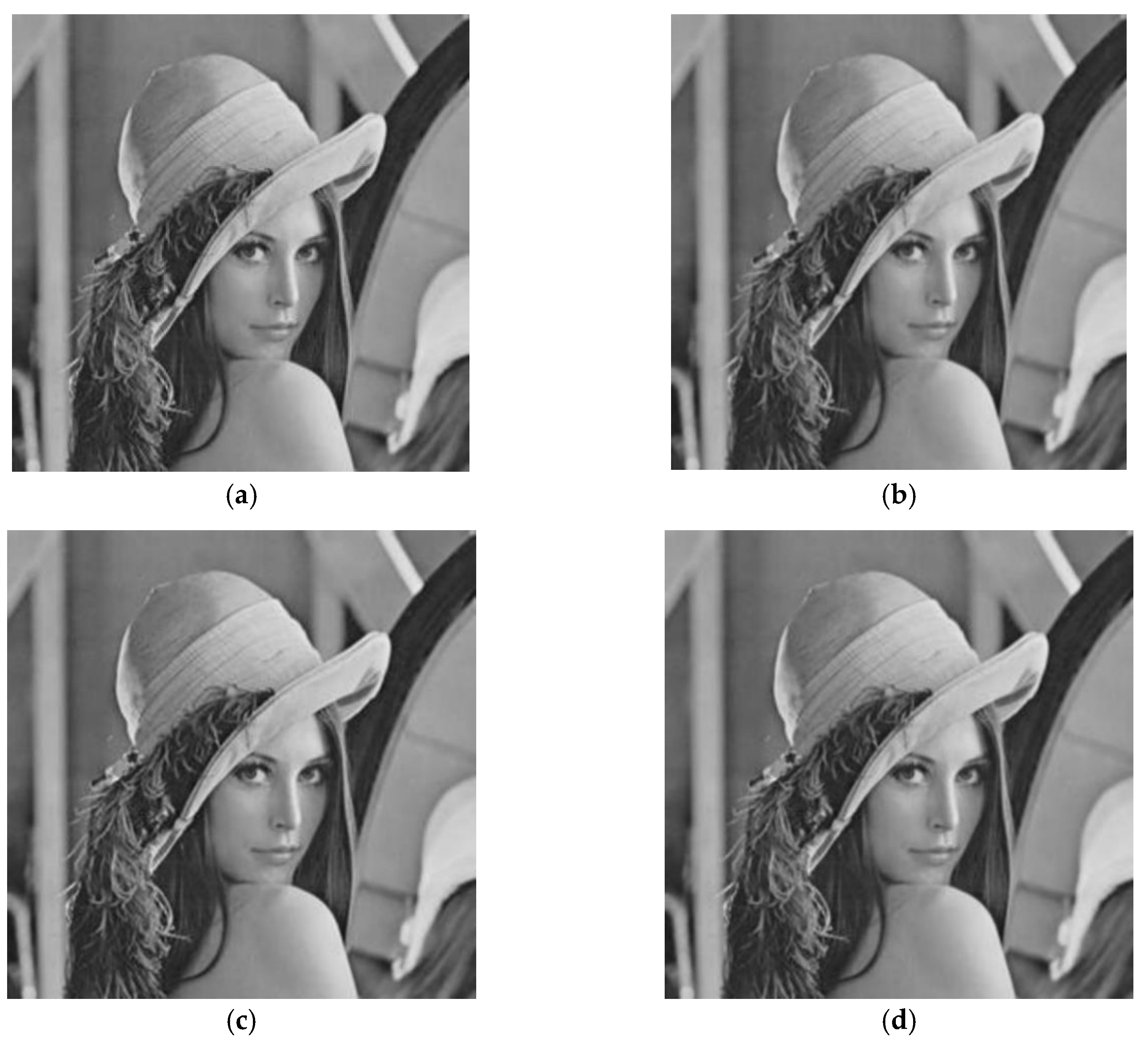
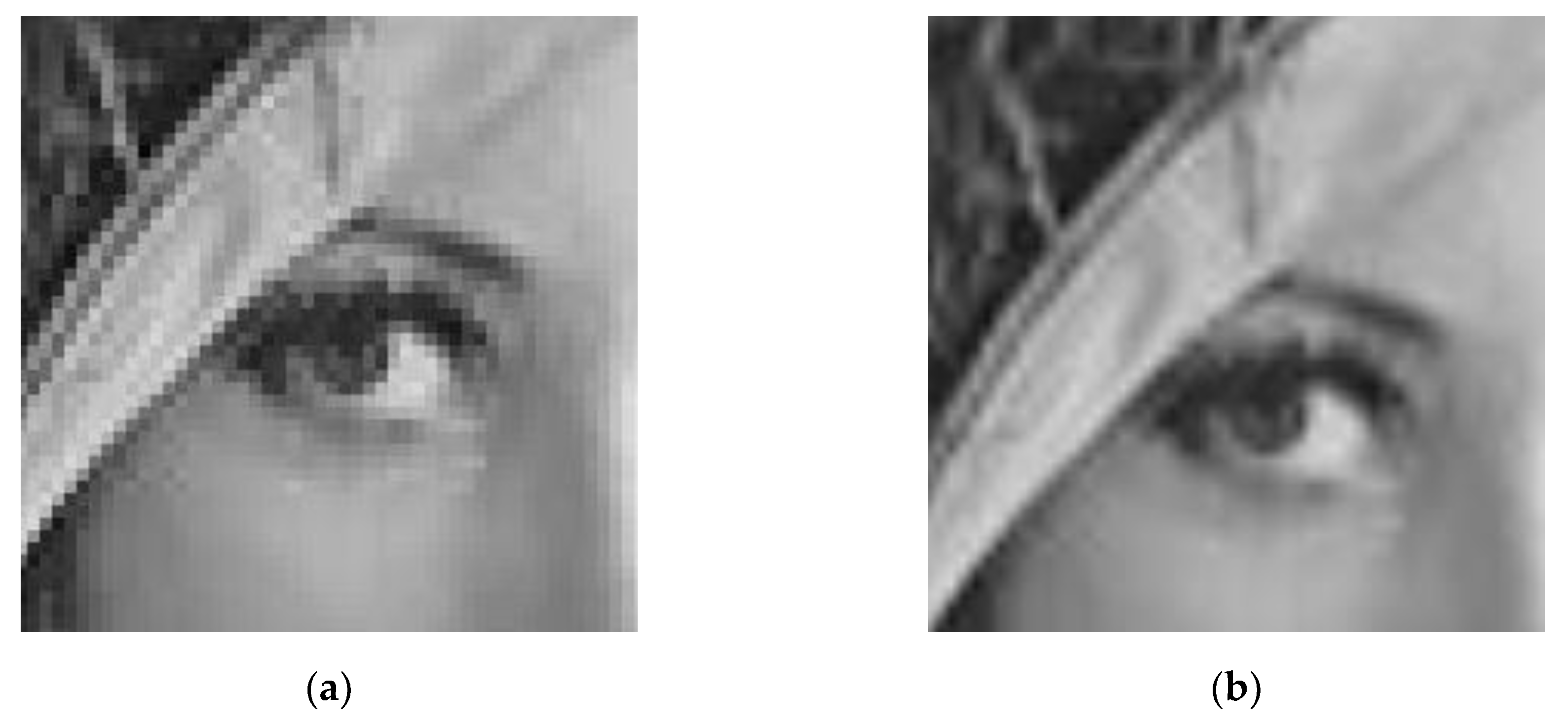
4. Numerical Examples

In this section, we provide some examples to illustrate how this method is implemented and its flexibility. The first example is given to demonstrate that the Thiele-like interpolation continued fractions with parameters are stable for the Runge function. The second example shows the interpolation with unattainable points in classical Thiele-type continued fractions rational interpolation. The third example is the multivariate Thiele-like rational interpolation continued fractions with parameters. To enrich the application of the proposed algorithm, we present an image zoom example based on parameterized bivariate Thiele-like rational interpolation continued fractions in the fourth example.

Example 1.

For the function$f(x_{})=\frac{1}{1+25x_{}^2}$, the higher-degree polynomial interpolation is unstable.

We can derive the classic Newton polynomial interpolation with the given data at points −1, −0.8, −0.6, −0.4, −0.2, 0:

$$\begin{array}{l}P=0.03846+0.1018(x+1)+0.26025(x+1)(x+0.8)+0.7916667(x+1)(x+0.8)(x+0.6)\\ +2.686979(x+1)(x+0.8)(x+0.6)(x+0.4)-6.36354(x+1)(x+0.8)(x+0.6)(x+0.4)(x+0.2)\end{array}$$

We can get the Thiele-type continued fractions interpolation:

$$R=\frac{1923}{5000}+\frac{x+1}{9.823182711}\begin{array}{c}\\ +\end{array}\frac{x+0.8}{-0.06018033}\begin{array}{c}\\ +\end{array}\frac{x+0.6}{-37.753208}\begin{array}{c}\\ +\end{array}\frac{x+0.4}{0.021847219}\begin{array}{c}\\ +\end{array}\frac{x+0.2}{-5883.58062}.$$

We can use Thiele-like interpolation continued fractions with parameters to calculate it. As the function has symmetry, we just discuss the condition within$[-1,0]$of the interpolation interval. If we set$[-0.8,0.05882]$as a virtual double point, we can get

$$\begin{array}{l}R=\frac{1923}{5000}+\frac{x+1}{\frac{509}{5000}}\begin{array}{c}\\ +\end{array}\frac{x+0.8}{c}\begin{array}{c}\\ +\end{array}\frac{x+0.8}{\frac{-1}{5(\mathrm{c}+\frac{1566193}{26025000})}}\begin{array}{c}\\ +\end{array}\frac{x+0.6}{\frac{-(26025000\mathrm{c}+1566193)(62787500\mathrm{c}+4111193)}{50000(32680893750\mathrm{c}+1793617763)}}\\ \begin{array}{c}\\ +\end{array}\frac{x+0.4}{\frac{-\left(24\right(32680893750\mathrm{c}+1793617763\left)\right(27478062500\mathrm{c}+1461475921\left)\right)}{2545(26025000\mathrm{c}+1566193)(16895932679\mathrm{c}+956527052)}}\\ \begin{array}{c}\\ +\end{array}\frac{x+0.2}{\frac{(16895932679\mathrm{c}+956527052)(844806165185\mathrm{c}+47828425248)}{8(32680893750\mathrm{c}+1793617763)(1689901538395\mathrm{c}+95660995792)}}\end{array}$$

As shown in

Table 2. Comparison table of different interpolation.

${\mathit{x}}_{\mathit{i}}$	$\mathit{f}({\mathit{x}}_{\mathit{i}})=\frac{1}{1+25{\mathit{x}}_{\mathit{i}}^2}$	$\mathbf{Newton}\mathbf{Interpolation}{\mathit{p}}_6(\mathit{x})$	Thiele Continued Fractions Interpolation	Thiele Continued Fractions Interpolation with c = 1	Thiele Continued Fractions Interpolation with c = −10
−1.00	0.03846	0.03846	0.03846000000	0.03846000000	0.03846000000
−0.96	0.04160	0.03298	0.04159488287	0.04159595868	0.04159595865
−0.90	0.04706	0.03770	0.04705547745	0.04705768836	0.04705768826
−0.86	0.05131	0.04534	0.05130475006	0.05130739205	0.05130739185
−0.80	0.05882	0.05882	0.05882000000	0.05882000000	0.05882000000
−0.76	0.06477	0.06763	0.06476367286	0.06476628712	0.06476628741
−0.70	0.07547	0.07971	0.07546947663	0.07547137553	0.07547137561
−0.66	0.08410	0.08737	0.08410290267	0.08410410847	0.08410410852
−0.60	0.10000	0.10000	0.09999999823	0.10000000000	0.10000000000
−0.56	0.11312	0.11071	0.11312302677	0.11312226113	0.11312226113
−0.50	0.13793	0.13338	0.13793269272	0.13793118870	0.13793118867
−0.46	0.15898	0.15487	0.15898409183	0.15898264914	0.15898264914
−0.40	0.2000	0.20000	0.19999998642	0.20000000000	0.20000000000
−0.36	0.23585	0.24042	0.23584678820	0.23584889034	0.23584889036
−0.30	0.30769	0.31883	0.30768550203	0.30769184706	0.30769184712
−0.26	0.37175	0.38372	0.37173857114	0.37174665711	0.37174665718
−0.20	0.50000	0.50000	0.49999990866	0.50000000000	0.50000000000
−0.16	0.60976	0.73720	0.60977966699	0.60975745619	0.60975745603
−0.10	0.80000	0.73720	0.80009647464	0.80000519086	0.80000519027
−0.06	0.91743	0.84193	0.91756721089	0.91743821176	0.91743821096
0.00	1.0000	1.00000	0.99999979851	1.00000000000	1.00000000000

, the Thiele-like interpolation continued fractions can perform better than the Newton polynomial interpolation with six points. However, these two methods cannot interpolate all of the interpolation data. The Thiele-like rational interpolation continued fractions with a parameter invariably satisfies the interpolation condition with different values of parameter $c$, and gives a better effect, and we also can get some new Thiele-like rational interpolation continued fractions formulas by selecting parameters. This is similar to the block-based Thiele-like blending rational interpolation [30]. We also can construct many other Thiele-type rational interpolation continued fractions using other virtual points or many parameters.

Example 2.

Given the following interpolation data in

Table 3. Interpolation data.

$i$	0	1	2
$x_i$	2	1	0
$f_i$	1	0	0

, the corresponding inverse difference table of Thiele-type continued fractions interpolation is shown in

Table 4. Table of inverse differences.

Nodes	0 Order Inverse Differences	1 Order Inverse Differences	2 Order Inverse Differences
2	1
1	0	1
0	0	2	−1

and

Table 5. Table of inverse differences with a parameter.

Nodes	0 Order Inverse Differences	1 Order Inverse Differences	2 Order Inverse Differences	3 Order Inverse Differences
2	1
2	1	$\lambda$
1	0	1	$\frac{1}{\lambda -1}$
0	0	2	$\frac{2}{\lambda -2}$	$3-\frac{2}{\lambda }-\lambda$

.

So, we can get the Thiele-type continued fractions rational interpolation:

$$r(x)=1+\frac{x-2}{1}\begin{array}{c}\\ +\end{array}\frac{x-1}{-1}=0.$$

As$r(x_0)=r(2)=0\ne 1$, we can see that$(2,1)$is a unique unattainable point. Following the algorithm in this paper, by adding multiple numbers of node$(2,1)$, the osculating interpolation which has a first-order derivative at point$(2,1)$, introducing parameter$\lambda (\lambda \ne 0)$, and constructing the inverse difference table shown in Table 5 above, we gain the corresponding Thiele-type osculatory rational interpolation:

$$R_2(x)=1+\frac{x-2}{\lambda }\begin{array}{c}\\ +\end{array}\frac{x-2}{\frac{1}{\lambda -1}}\begin{array}{c}\\ +\end{array}\frac{x-1}{3-\frac{2}{\lambda }-\lambda }.$$

It is easy to verify that

$$R_2(x_i)=f_i\begin{array}{cc}& (i=0,1,2)\end{array}.$$

So, by choosing the different value of parameter$\lambda$, the function$R_2(x)$invariably satisfies the given interpolation data. Meantime, this method can well solve this kind of special interpolation problem, and it is easy to construct and calculate. In addition, the function$R_2(x)$can be converted into many other rational interpolation functions. For example, we can choose the following functions:If we choose$\lambda =-3$, we can get

$$R_2(x)=1+\frac{x-2}{-3}\begin{array}{c}\\ +\end{array}\frac{x-2}{-\frac{1}{4}}\begin{array}{c}\\ +\end{array}\frac{x-1}{\frac{20}{3}}.$$

If we choose$\lambda =80$, we can get

$$R_2(x)=1-\frac{x-2}{-80}\begin{array}{c}\\ +\end{array}\frac{x-2}{\frac{40x}{3081}-\frac{1}{39}}.$$

(57)

As can be seen from Figure 1, both functions satisfy the interpolation condition. We can choose other values of the parameters$\lambda (\lambda \ne 0)$, and the function$R_3(x)$can change into other functions.

Example 3.

The interpolation data are given in

Table 6. Interpolation data.

$({\mathit{x}}_{\mathit{i}},{\mathit{y}}_{\mathit{j}})$	${\mathit{x}}_0=0$	${\mathit{x}}_1=0.5$	${\mathit{x}}_2=1$
$y_0=0$	2	2.3	2.5
$y_1=0.5$	1.8	2	2.1
$y_1=1$	1.5	1.55	1.5

.

We can get the bivariate Thiele-type blending rational interpolation using the method presented in [1]:

$$R(x,y)=2-\frac{y}{\frac{5}{2}+\frac{y-0.5}{-1}}+\frac{x}{\frac{5}{3}+\frac{y}{\frac{3}{5}+\frac{y-0.5}{-\frac{25}{24}}}}\begin{array}{c}\\ +\end{array}\frac{x-0.5}{\frac{3}{2}+\frac{y}{-\frac{5}{9}+\frac{y-0.5}{-\frac{9}{2}}}}.$$

Following Algorithm 3 in this paper, we add the multiplicity of point$(0,0,2)$and construct the osculating interpolation which has its first-order derivative at point$(0,0,2)$by introducing parameter$\lambda$:

$$R^{(0)}(x,y)=2+\frac{y}{\lambda +\frac{y}{\frac{-1}{2\lambda +5}+\frac{y-0.5}{\frac{-(2\lambda +5\left)\right(\lambda +2)}{2(\lambda +3)}}}}+\frac{x}{\frac{5}{3}+\frac{y}{\frac{3}{5}+\frac{y-0.5}{-\frac{25}{24}}}}\begin{array}{c}\\ +\end{array}\frac{x-0.5}{\frac{3}{2}+\frac{y}{-\frac{5}{9}+\frac{y-0.5}{-\frac{9}{2}}}}.$$

It is easy to verify that the function$R_2(x)$invariably satisfies the given interpolation data with the different value of parameter$\lambda$, i.e.,

$$R(x_i,y_j)=R^{(0)}(x_i,y_j)=f_{ij}(i,j=0,1,2).$$

We can modify the bivariate blending rational interpolation by selecting parameters, but$R(x,y)$cannot, so our method gives a new choice for the application, and it gives a new method for studying the rational interpolation theory.

Example 4.

Image interpolation is an important method in pixel level image processing, the interpolated data are often regarded as a certain interpolation kernel and a linear combination of the input image pixels in traditional methods. Due to the influence of light, natural background and image texture characteristics, generally speaking, the adjacent pixels of an image are not a simple linear relationship. In order to obtain more effective and better visual results, many nonlinear methods have been proposed for the image interpolation in the literature. To enrich the application of the proposed parameterized bivariate Thiele-like rational interpolation continued fractions algorithm, we take an image zoom as an example. We choose$\lambda =1$, the performances of the proposed parameterized Thiele-like continued fraction rational interpolation method can be deduced from image interpolation process. In our experiment, we take the image ”Lenna” as the test image as shown in Figure 2. The original image is resized by a factor 2 (see Figure 3) with four image interpolation methods. The experiment results demonstrate that the zoomed images do not have obvious jagged edges with the proposed parameterized Thiele-like continued fraction rational interpolation method, so the proposed algorithm can be used for image interpolation processing effectively. It is obvious that our new method is implemented without producing the so-called mosaics or blocky effect, and the results maintain clearness of the image, including edges, and the details are maintained well, hence, it offers more detailed information. From Figure 4 , we can see, when the image is enlarged by a larger factor, the new proposed algorithm still has better visual performance.

5. Conclusions and Future Work

In this paper, by strategically selecting the multiplicity of the interpolation nodes, we have developed many types of univariate and bivariate Thiele-like rational interpolation continued fractions with parameters. We also discussed the interpolant algorithms, interpolant theorems, and dual interpolation. The new kinds of Thiele-like rational interpolation continued fractions are easy to use and extend the theoretical research and application of the rational interpolation functions. The value of the interpolation function can be changed at any point in the interpolant region under unaltered interpolant points by selecting appropriate parameters; therefore, it can be used to design a curve or surface. Based on the geometric design needs, it can alter the shape of curves or surfaces to satisfy actual needs. However, it is still a complicated problem. The selection of proper parameters and construction of an appropriate interpolation method for actual geometric design requirements are a very practical and interesting problem, and we will study it in the future. Further research on the following aspects will be summarized in our next study:

• How to select appropriate parameters and suitably alter the shape of the curves or surfaces according to actual requirements.
• The geometric properties of curves/surfaces based on the Thiele-like rational interpolation continued fractions function with parameters.
• How to design geometric modeling using Thiele-like rational interpolation continued fractions functions with parameters.
• The proposed Thiele-like rational interpolation continued fractions with parameters algorithm can be implemented in other pixel level image processing, such as image inpainting, removal of salt and pepper noise, image rotation, image super-resolution reconstruction, image metamorphosis and image upscaling.
• How to generalize the proposed algorithms to lacunary rational interpolants, rational interpolants over triangular grids.

To conclude, by using of the Sampson generalized inverse, it is not complicated to generalize the Thiele-like rational interpolation continued fractions algorithms with parameters to vector-valued cases or matrix-valued cases [1,2].

References

1. Tan, J. Theory of Continued Fractions and Its Applications; Science Publishers: Beijing, China, 2007. [Google Scholar]
2. Wang, R.; Zhu, G. Approximation of Rational Interpolation and Its Application; Science Publishers: Beijing, China, 2004. [Google Scholar]
3. Kuchmins’ka, K.; Vonza, S. On Newton-Thiele-like Interpolating Formula. Commun. Anal. Theory Contin. Fractions 2000, 8, 74–79. [Google Scholar]
4. Pahirya, M.; Svyda, T. Problem of Interpolation of Functions by Two-Dimensional Continued Fractions. Ukrai. Math. J. 2006, 58, 954–966. [Google Scholar] [CrossRef]
5. Li, S.; Dong, Y. Viscovatov-Like Algorithm of Thiele-Newton’s Blending Expansion for a Bivariate Function. Mathematics 2019, 7, 696. [Google Scholar] [CrossRef] [Green Version]
6. Cuyt, A.; Celis, O. Multivariate Data Fitting With Error Control. Bit Numer. Math. 2019, 59, 35–55. [Google Scholar] [CrossRef]
7. Li, G.; Zhang, X.; Yang, H. Numerical Analysis, Circuit Simulation, And Control Synchronization of Fractional-Order Unified Chaotic System. Mathematics 2019, 7, 1077. [Google Scholar] [CrossRef] [Green Version]
8. Xu, Q.; Liu, Z. Scattered Data Interpolation and Approximation with Truncated Exponential Radial Basis Function. Mathematics 2019, 7, 1101. [Google Scholar] [CrossRef] [Green Version]
9. Massopust, P. Non-Stationary Fractal Interpolation. Mathematics 2019, 7, 666. [Google Scholar] [CrossRef] [Green Version]
10. Akal, C.; Lukashov, A. Newton-Padé Approximations for Multivariate Functions. Appl. Math. Comput. 2018, 334, 367–374. [Google Scholar] [CrossRef]
11. Cuyt, A.; Verdonk, B. General Order Newton-Padé Approximants for Multivariate Functions. Numer. Math. 1984, 43, 293–307. [Google Scholar] [CrossRef]
12. Ravi, M.S. Geometric Methods in Rational Interpolation Theory. Linear Algebra Appl. 1997, 258, 159–168. [Google Scholar] [CrossRef] [Green Version]
13. Bertrand, F.; Calvi, J. The Newton Product of Polynomial Projectors Part 1: Construction and Algebraic Properties. Int. J. Math. 2019, 30, 1950030. [Google Scholar] [CrossRef]
14. Akal, C.; Lukashov, A. Scale of Mean Value Multivariate Padé Interpolations. Filomat 2017, 31, 1123–1128. [Google Scholar] [CrossRef]
15. Li, H.B.; Song, M.Y.; Zhong, E.J.; Gu, X.M. Numerical Gradient Schemes for Heat Equations Based on the Collocation Polynomial and Hermite Interpolation. Mathematics 2019, 7, 93. [Google Scholar] [CrossRef] [Green Version]
16. Yu, K.; Wang, C.; Yang, S.; Lu, Z.; Zhao, D. An Effective Directional Residual Interpolation Algorithm for Color Image Demosaicking. Appl. Sci. 2018, 8, 680. [Google Scholar] [CrossRef] [Green Version]
17. Zhou, X.; Wang, C.; Zhang, Z.; Fu, Q. Interpolation Filter Design Based on All-Phase DST And Its Application to Image Demosaicking. Information 2018, 9, 206. [Google Scholar] [CrossRef] [Green Version]
18. Min, H.; Jia, W.; Zhao, Y. LATE: A Level Set Method Based on Local Approximation of Taylor Expansion for Segmenting Intensity Inhomogeneous Images. IEEE Trans. Image Process. 2018, 27, 5016–5031. [Google Scholar] [CrossRef]
19. He, L.; Tan, J.; Xing, Y.; Hu, M.; Xie, C. Super-Resolution Reconstruction Based on Continued Fractions Interpolation Kernel in The Polar Coordinates. J. Electron. Imaging 2018, 27, 043035. [Google Scholar] [CrossRef]
20. He, L.; Tan, J.; Su, Z.; Luo, X.; Xie, C. Super-resolution by polar Newton-Thiele’s rational kernel in centralized sparsity paradigm. Signal Process. Image Commun. 2015, 31, 86–99. [Google Scholar] [CrossRef]
21. Yao, X.; Zhang, Y.; Bao, F.; Liu, F.; Zhang, M. The Blending Interpolation Algorithm Based on Image Features. Multimed. Tools Appl. 2018, 77, 1971–1995. [Google Scholar] [CrossRef]
22. Zhang, Y.; Fan, Q.; Bao, F.; Liu, Y.; Zhang, C. Single-Image Super-Resolution Based on Rational Fractal Interpolation. IEEE Trans. Image Process. 2018, 27, 3782–3797. [Google Scholar]
23. Ahn, H.E.; Jeong, J.; Kim, J.W.; Kwon, S.; Yoo, J. A Fast 4K Video Frame Interpolation Using a Multi-Scale Optical Flow Reconstruction Network. Symmetry 2019, 11, 1251. [Google Scholar] [CrossRef] [Green Version]
24. Wei, X.; Wu, Y.; Dong, F.; Zhang, J.; Sun, S. Developing an Image Manipulation Detection Algorithm Based on Edge Detection and Faster R-CNN. Symmetry 2019, 11, 1223. [Google Scholar] [CrossRef] [Green Version]
25. Zhang, Y.; Bao, F.; Zhang, M. A Rational Interpolation Surface Model and Visualization Constraint. Sci. Sin. Math. 2014, 44, 729–740. [Google Scholar] [CrossRef]
26. Zhang, Y.; Bao, X.; Zhang, M.; Duan, Q. A Weighted Bivariate Blending Rational Interpolation Function and Visualization Control. J Comput. Anal. Appl. 2012, 14, 1303–1320. [Google Scholar]
27. Zou, L.; Tang, S. New Approach to Bivariate Blending Rational Interpolants. Chin. Q. J. Math. 2011, 26, 280–284. [Google Scholar]
28. Zou, L.; Tang, S. General Structure of Block-Based Interpolational Function. Commun. Math. Res. 2012, 28, 193–208. [Google Scholar]
29. Zou, L.; Tang, S. A New Approach to General Interpolation Formulae for Bivariate Interpolation. Abstr. Appl. Anal. 2014, 2014, 421635. [Google Scholar] [CrossRef]
30. Zhao, Q.; Tan, Q. Block-based Thiele-like Blending Rational Interpolation. J. Comput. Appl. Math. 2006, 195, 312–325. [Google Scholar] [CrossRef] [Green Version]
31. Zhu, X.; Zhu, G. A Study of the Existence of Vector Valued Rational Interpolation. J. Inf. Comput. Sci. 2005, 2, 631–640. [Google Scholar]
32. Zhu, X. Research and Application of Rational Function Interpolation. Ph.D. Thesis, University of Science and Technology of China, Hefei, China, 2002. [Google Scholar]
33. Zou, L.; Song, L.; Wang, X.; Huang, Q.; Chen, Y.; Tang, C.; Zhang, C. Univariate Thiele Type Continued Fractions Rational Interpolation with Parameters. In International Conference on Intelligent Computing; Springer: Cham, Switzerland, 2019; pp. 399–410. [Google Scholar]
34. Huang, D.; Huang, Z.; Hussain, A. Intelligent Computing Methodologies; Springer Science and Business Media LLC: Berlin/Heidelberg, Germany, 2019. [Google Scholar]
35. Li, C.W.; Zhu, X.L.; Pan, Y.L. A Study of The Unattainable Point for Rational Interpolation. Coll. Math. 2010, 26, 50–55. [Google Scholar]
36. Zhao, Q.; Tan, Q. Successive Newton-Thiele’s Rational Interpolation. J. Inf. Comput. Sci. 2005, 2, 295–301. [Google Scholar]
37. Zhao, Q.; Tan, Q. Block-based Newton-like Blending Rational Interpolation. J. Comput. Math. 2006, 24, 515–526. [Google Scholar]
38. Siemazko, W. Thiele-type Branched Continued Fractions for Two Variable Functions. J. Comput. Appl. Math. 1983, 9, 137–153. [Google Scholar] [CrossRef] [Green Version]
Figure 1. (a) Graph of R 2 ( x ) with λ = 3 , (b) graph of R 2 ( x ) with λ = 80 .
Mathematics 08 00071 g001
Figure 2. The original Lenna Image.
Mathematics 08 00071 g002
Figure 3. The zoomed images by factor 2 based on four different interpolant methods. (a) The zoomed images by factor 2 based on the nearest-neighbor interpolation method, (b) the zoomed images by factor 2 based on the bilinear interpolation, (c) the zoomed images by factor 2 based on the bicubic interpolation, (d) the zoomed images by factor 2 based on the proposed method.
Mathematics 08 00071 g003
Figure 4. Comparison of eye effects of the nearest neighbor interpolation and the proposed rational interpolation. (a) The zoomed images by factor 4 based on the nearest-neighbor interpolation method, (b) the zoomed images by factor 4 based on the proposed method.
Mathematics 08 00071 g004