Article

Mixed Generalized Multiscale Finite Element Method for Darcy-Forchheimer Model

1
Multiscale Model Reduction Laboratory, North-Eastern Federal University, 677980 Yakutsk, Republic of Sakha (Yakutia), Russia
2
School of Mathematics and Computational Science, Xiangtan University, Xiangtan 411105, China
3
Hunan Key Laboratory for Computation and Simulation in Science and Engineering, Xiangtan 411105, China
4
Key Laboratory of Intelligent Computing Information Processing of Ministry of Education, Xiangtan 411105, China
5
Institute for Scientific Computation, Texas A&M University, College Station, TX 77843-3368, USA
6
Department of Computational Technologies, North-Eastern Federal University, 677980 Yakutsk, Republic of Sakha (Yakutia), Russia
7
Department of Mathematics, The Chinese University of Hong Kong (CUHK), Hong Kong, China
*
Author to whom correspondence should be addressed.
Mathematics 2019, 7(12), 1212; https://doi.org/10.3390/math7121212
Submission received: 7 October 2019 / Revised: 3 December 2019 / Accepted: 5 December 2019 / Published: 10 December 2019
(This article belongs to the Special Issue Computational Mathematics, Algorithms, and Data Processing)

Abstract

:
In this paper, the solution of the Darcy-Forchheimer model in high contrast heterogeneous media is studied. This problem is solved by a mixed finite element method (MFEM) on a fine grid (the reference solution), where the pressure is approximated by piecewise constant elements; meanwhile, the velocity is discretized by the lowest order Raviart-Thomas elements. The solution on a coarse grid is performed by using the mixed generalized multiscale finite element method (mixed GMsFEM). The nonlinear equation can be solved by the well known Picard iteration. Several numerical experiments are presented in a two-dimensional heterogeneous domain to show the good applicability of the proposed multiscale method.

1. Introduction

The Darcy-Forchheimer equation is commonly used for describing the high velocity flow near oil and gas wellbores and fractures, which is a correction formula of the well known Darcy’s law by supplementing a nonlinear velocity quantity as follows:
μ k 1 u + β ρ u u + p = 0 ,
where μ , k , ρ and β represent the viscosity, the permeability, the density, and the dynamic viscosity coefficient of the fluid, respectively. β is also mentioned as the Forchheimer coefficient, whose values stand for the nonlinear intensity. In contrast, Darcy’s law, which is valid for the extremely small velocity case, is usually used to show the linear relationship between the velocity vector u and the pressure gradient p . The Darcy-Forchheimer model can be obtained by coupling Equation (1) with the following conservation law equation:
· u = f .
In recent years, the Darcy-Forchheimer model has been studied by many researchers within numerical discretized methods. Girault et al. in [1] proved the existence and uniqueness of the solution of the Darcy-Forchheimer model. Then, they considered mixed finite element methods by piecewise constant and nonconforming Crouzeix-Raviart elements to approximate the velocity and the pressure, respectively. Park in [2] gave a mixed finite element method (MFEM) for generalized Darcy-Forchheimer flow. Pan et al. in [3] presented an MFEM to approximate the velocity based on the Raviart–Thomas element or the Brezzi–Douglas–Marini element and piecewise constant for the pressure of the Darcy-Forchheimer model. Rui et al. in [4] published a block-centered finite difference method (BCFDM) for the Darcy-Forchheimer model. The authors in [5] established a BCFDM for the Darcy-Forchheimer model with variable parameter β ( x ) . Rui and Liu in [6] introduced a two level BCFDM for the Darcy-Forchheimer model. Huang, Chen, and Rui in [7] designed a nonlinear multigrid method for the two-dimensional Darcy-Forchheimer model with a Peaceman–Rachford-type iteration as a smoother and proposed a better choice of the parameter used in the splitting. We point out that the constructed multigrid method with an almost linear computational cost is convergent independent of the critical parameters.
To solve the problem in heterogeneous media, a very fine mesh should be used for solving a heterogeneity scale problem, which results to a large number of degrees of freedom. For dimension reduction and fast solvers of such problems, some model reduction techniques are needed. In [8], the authors introduced the mixed multiscale finite element methods and presented the main convergence results for the solution of second order elliptic equations with heterogeneous coefficients, which oscillate rapidly. Mixed multiscale finite element methods are widely used for solving the reservoir simulation problems [9,10,11]. In [12,13,14], we developed a mixed generalized multiscale finite element method (GMsFEM), where we enriched a multiscale space by new degrees of freedom, which was obtained by solving local spectral problems on the snapshot space.
In this paper, we consider a solution of the Darcy-Forchheimer model in heterogeneous media. We construct an efficient algorithm of the mixed generalized multiscale finite element method to make an approximation of the problem on the coarse grid. The construction is based on solving the local problems for calculating multiscale basis functions of the velocity. Meanwhile, we use piecewise constant elements to approximate the pressure. In the mixed formulation, we firstly define a snapshot space, which provides a solution space in each local area. Then we solve the local spectral problem in the snapshot space to find out multiscale basis functions. We use the Picard iteration to address the non-linearity when solving the problems on the multiscale spaces [15,16]. Note that when constructing multiscale basis functions, we do not take into account the nonlinear part of the Darcy-Forchheimer equation.
The remainder of this article is organized as follows: The model problem and its weak formulation in mixed form and the discrete weak formulation are demonstrated in Section 2. The fine grid approximation and coarse gird approximation are presented in Section 3 and Section 4, respectively. Some numerical experiments using our mixed generalized multiscale finite element method are carried out in Section 5 to verify the efficiency of the presented method. Finally, conclusions and further ideas are presented in Section 6.

2. Mathematical Model

We consider the steady state Darcy-Forchheimer model to describe a single phase fluid flow in a heterogeneous porous medium.
μ k 1 ( x ) u + β ( x ) ρ | u | u + p = 0 , x Ω , · u = f , x Ω ,
where Ω R 2 is a bounded domain and Ω is Lipschitz continuous; v = v , v 1 2 , · , · denotes the L 2 inner product; k and β are the heterogeneous permeability and the heterogeneous non-Darcy coefficient, respectively.
Complemented with Dirichlet boundary condition,
p = f D , x Ω .
Without loss of generality, we suppose that f D = 0 , namely the homogeneous Dirichlet boundary condition. Then, we get the following problem:
μ k 1 ( x ) u + β ( x ) ρ | u | u + p = 0 , x Ω , · u = f , x Ω , p = 0 , x Ω .
Remark 1.
The boundary condition (4) can be replaced by the Neumann boundary condition,
u · n = f N , x Ω , .
f and f N should satisfy the compatibility condition by the Gauss theorem,
Ω f x d x = Ω f N s d s .

3. Fine Grid Approximation

In this section, mixed finite element methods have been borrowed to handle Problem (5) in the fine grid. Here, we use the standard Sobolev spaces notation to define the function spaces and their norms as follows:
V = v L 3 ( Ω ) 2 ; · v L 2 ( Ω ) , u V = v 0 , 3 , Ω + · v 0 , 2 , Ω , v V .
Q = L 2 ( Ω ) , q Q = q 0 , 2 , Ω , q Q .
Then, we obtain the following variational formulation: find ( u , p ) V × Q such that:
Ω μ k 1 ( x ) u v d x + Ω β ( x ) ρ | u | u v d x Ω p · v d x = 0 , v V , Ω q · u d x = Ω f q d x , q Q .
The variational formulation (8) and the problem (5) are equivalent by the following Green’s formula:
Ω p v d x = Ω p · v d x + Ω p v · n d s , v V .
Let Ω be a polygon in two dimensions, which can be entirely covered by a shape regular decomposition T h , in the sense of Ciarlet [17], into triangles, with h being the maximum diameter of the elements of the triangles. Therefore, T h is a family of conforming triangulations of Ω ¯ ,
Ω ¯ = T T h T .
Here, we discretize the velocity u in the lowest order Raviart–Thomas space:
Given a simplex T R 2 , the local Raviart–Thomas space of order k 0 is defined by:
R T k ( T ) = P k ( T ) 2 + x P k ( T ) ,
where P k denotes the set of all polynomials in two variables of degree k . Then, we can get the lowest order global Raviart–Thomas space, which is the conforming finite element space of the velocity u :
V h = R T 0 Ω = v V : v | T R T 0 ( T ) T T h .
The pressure p is approximated in the following piecewise constant space:
Q h = q L 2 Ω : q | T P 0 T T h .
Then, we can obtain the discrete weak formulation of (8): find a pair u h , p h V h × Q h :
Ω μ k 1 ( x ) u h v h d x + Ω β ( x ) ρ | u h | u h v h d x Ω p h · v h d x = 0 , v h V h , Ω q h · u h d x = Ω f q h d x , q h Q h .
In [3], the authors demonstrated the existence and uniqueness of the continuous problem and the discrete problem, respectively. Moreover, if T h is quasi-uniform and u , p W s , 3 ( Ω ) 2 × W s , 3 2 ( Ω ) , then the following error estimates can be proven; see ([3], Theorem 4.4) for details:
u u h 0 , 2 2 + u u h 0 , 3 3 C h 2 s , 1 s k + 1 ,
p p h 0 , 2 C h s , 1 s k + 1 .
where W s , p ( Ω ) is the standard Sobolev space of index ( s , p ) , where s is a nonnegative integer and p 1 .
W s , p ( Ω ) = v L p ( Ω ) : D α v L p ( Ω ) for all | α | s ,
where D α v is the weak derivative of v; see the details in [18].
Let:
u h = i = 1 m 1 u i ξ i , p h = i = 1 m 2 p i θ i ,
where u = [ u 1 , u 2 , , u m 1 ] T , p = [ p 1 , p 2 , , p m 2 ] T are the coefficients of the finite element approximations with m 1 , m 2 dimensions, in terms of a basis ξ of the velocity and a basis θ of the pressure, respectively.
We apply the Picard iteration for solving the resulting discrete nonlinear system.
Find u h n + 1 V h , p h n + 1 Q h with an arbitrary initial guess u h 0 V h , such that:
Ω μ k 1 ( x ) u h n + 1 v h d x + Ω β ( x ) ρ | u h n | u h n + 1 v h d x Ω p h n + 1 · v h d x = 0 , v h V h , Ω q h · u h n + 1 d x = Ω f q h d x , q h Q h .
We rewrite the iteration (15) into the following matrix form.
A ( u h n ) B T B 0 u h n + 1 p h n + 1 = 0 F ,
where A ( u h ) is the matrix associated with the term:
Ω μ k 1 ( x ) u h v h d x + Ω β ( x ) ρ | u h | u h v h d x ,
where B is the matrix corresponding to Ω q h · u h d x , and F is the vector associated with the linear functional Ω f q h d x .
In the practical implementation, we use the following termination criterion to control the iteration,
max ( r u , r p ) < t o l ,
where:
r u = μ k 1 ( x ) u h n + 1 + β ( x ) ρ | u h n + 1 | u h n + 1 + p h n + 1 0 , r p = f · u h n + 1 0 / f 0 , when f 0 0 , f · u h n + 1 0 , when f 0 = 0 .

4. Coarse Grid Approximation

In this section, we describe the construction of the approximation on a coarse grid using the mixed generalized multiscale finite element method (mixed GMsFEM). We construct a square uniform coarse grid T H for the computational domain Ω with a coarse grid size H; E H = i = 1 N E E i is the set of all facets of a coarse mesh, and N E 
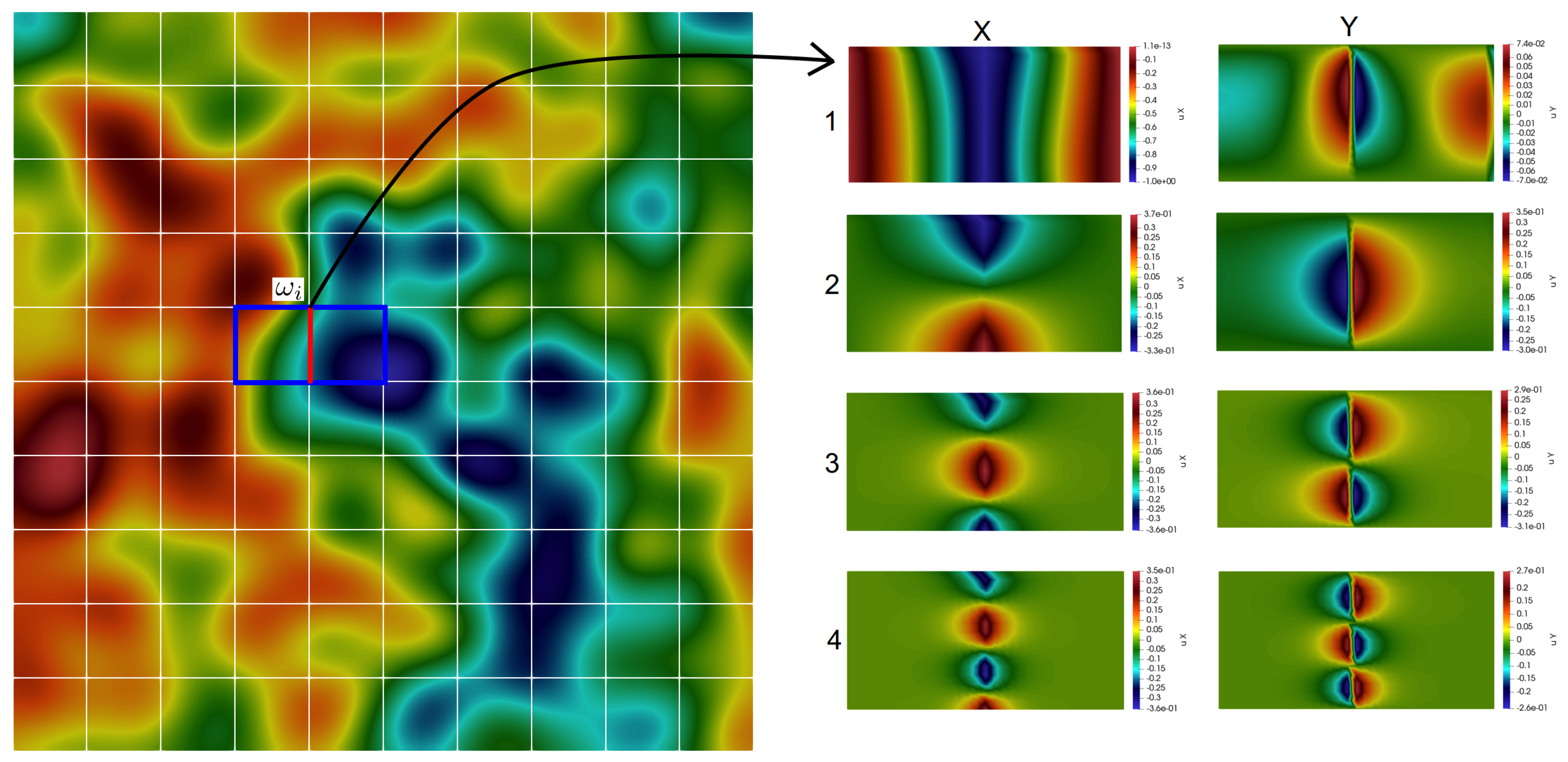
is the number of facets of a coarse mesh. To construct the multiscale basis function, we build a uniform triangular fine grid, which is obtained by refinement of a coarse grid. In the mixed GMsFEM, we compute the multiscale basis functions for the velocity in the local domains ω i that correspond to the coarse edge E i E H (Figure 1).
ω i = j { K j T H | E i K j } ,
where K j is the coarse grid cell, which is equal to a square element of T H .
We build a multiscale space for the velocity u m s V m s :
V m s = span { ψ 1 , , ψ M ω i · N E } ,
where ψ i are the multiscale basis functions, which are calculated in the local domain ω i and M ω i is the number of basis functions in each local domain. For pressure, we use the space Q m s of piecewise constant functions on the coarse cells.
We start with constructing a snapshot space in the local domain ω i and then make an approximation on the coarse grid using the solution of the local spectral problem on the snapshot space. The snapshot space is obtained by solving the next local problem in ω i : find ( ϕ j , η ) V h ω i × Q h ω i such that:
ω i k 1 ϕ j i v d x ω i η · v d x = 0 , v V h ω i , ω i r · ϕ j i d x = ω i c j r d x , r Q h ω i ,
with boundary condition:
ϕ j i · n = 0 , x ω i ,
where n is the unit exterior normal vector to the boundary ω i .
On the fine facet e j , we apply an additional boundary condition:
ϕ j i · n = δ i j , x e j ,
where j = 1 , , J ω i is the number of the fine facets e j on which we define the boundary condition (20), c j = | e j | S ω i is chosen by the compatibility condition ω i ϕ j i · n = · ϕ j i , | e j | presents the length of the fine grid facet e j , and S ω i denotes the volume of the local domain ω i . Here, J ω i is the number of fine grid edges e j on E i , E i = j = 1 J ω i e j , and δ i j is a piecewise constant function defined on E i , which takes the value of one on e j and zero on each other edge of the fine grid.
Therefore, we can define the snapshot space in each local domain ω i :
V s n a p i = span { ϕ 1 i , , ϕ J i i } .
To compute a multiscale basis function, we solve a local spectral problem in each local domain ω i . The spectral problem allows us to find the most important characteristics of the problem. Then, we use multiscale basis functions to define the multiscale space to get an approximation on the coarse grid. In each ω i , we solve the spectral problem on V s n a p i :
A ˜ ω i ψ ˜ l ω i = λ l S ˜ ω i ψ ˜ l ω i , A ˜ ω i = R ω i A ω i ( R ω i ) T , S ˜ ω i = R ω i S ω i ( R ω i ) T ,
where:
( R ω i ) T = [ ϕ 1 i , , ϕ J ω i i ] ,
and:
A ω i = [ a m n ω i ] , a m n ω i = a ω i ( ϕ m , ϕ n ) = E i k 1 ( ϕ m · n ) ( ϕ n · n ) d s ,
S ω i = [ s m n ω i ] , s m n ω i = s ω i ( ϕ m , ϕ n ) = ω i k 1 ϕ m ϕ n d x + ω i · ϕ m · ϕ n d x .
For construction of the multiscale space, we select the first M ω i smallest eigenvalues and take the corresponding eigenvectors ψ l ω i = ( R ω i ) T ψ ˜ l ω i as basis functions ( l = 1 , 2 , , M ω i ). We note that the presented spectral decomposition in the snapshot space is motivated by theoretical analysis (see Theorem 4.3 in [12]). Moreover, the oversampling techniques can be used for the construction of the multiscale basis functions to enhance the accuracy of mixed GMsFEM. The main idea of oversampling techniques is to introduce a small dimensional snapshot space using the POD (proper orthogonal decomposition) approach, where snapshot vectors are constructed in larger regions that contain the interfaces of two adjacent coarse blocks [12].
Remark 2.
For the construction of the multiscale basis functions, we can use other types of spectral problems (see [12,19]). For example, we can solve the following spectral problem:
S ˜ ω i ψ ˜ l ω i = μ l ψ ˜ l ω i , S ˜ ω i = R ω i S ω i ( R ω i ) T ,
with:
S ω i = [ s m n ω i ] , s m n ω i = s ω i ( ϕ m , ϕ n ) = ω i k 1 ϕ m ϕ n d x ,
on the snapshot space and taking eigenvectors corresponding to the largest eigenvalues as a multiscale basis functions ( λ l = 1 / μ l ).
Additionally, we calculate the first basis function by the solution of the following local problem in the domain ω i : find ( χ ω i , η ) V h ω i × Q h ω i such that:
ω i k 1 χ ω i v d x ω i η · v d x = 0 , v V h ω i , ω i r · χ ω i d x = ω i c r d x , r Q h ω i ,
with the following boundary conditions:
χ ω i · n = 0 , x ω i , χ ω i · n = 1 , x E i ,
where c = | E i | S ω i , | E i | is the length of coarse facet E i .
Finally, we obtain the following multiscale space for velocity:
V m s = span { χ ω i , ψ l ω i , 1 l M ω i , 1 i N E } .
The illustration of the local multiscale basis functions with an additional basis are presented in Figure 1.
For the construction of the coarse grid system, we define a projection matrix:
R = R u 0 0 R p , R u = [ R u , 1 , , R u , N E ] T ,
where ( R u , i ) T = [ χ ω i , ψ 1 ω i , , ψ M ω i ω i ] and R p is the projection matrix for pressure, where we set one for each fine grid cell in the current coarse grid cell. Here, N E is the number of facets of the coarse grid, and M ω i is the number of multiscale basis functions in local domain ω i .
We use the constructed multiscale space and write the approximation in the coarse grid in matrix form:
A c k B c T B c 0 u c k + 1 p c k + 1 = 0 F c ,
where:
A c k = R u A k R u T , B c = R u B R p T , F c = R p F ,
and finally, we reconstruct the solution on the fine grid u m s k + 1 = R u T u c k + 1 .

5. Numerical Results

In this section, we present several numerical results of the Darcy-Forchheimer model in the domain Ω = [ 0 , 1 ] 2 . We used a structured 160 × 160 fine grid with 77,120 edges and 51,200 cells (triangles) and a 10 × 10 coarse grid with 220 edges and 100 cells (see Figure 2).
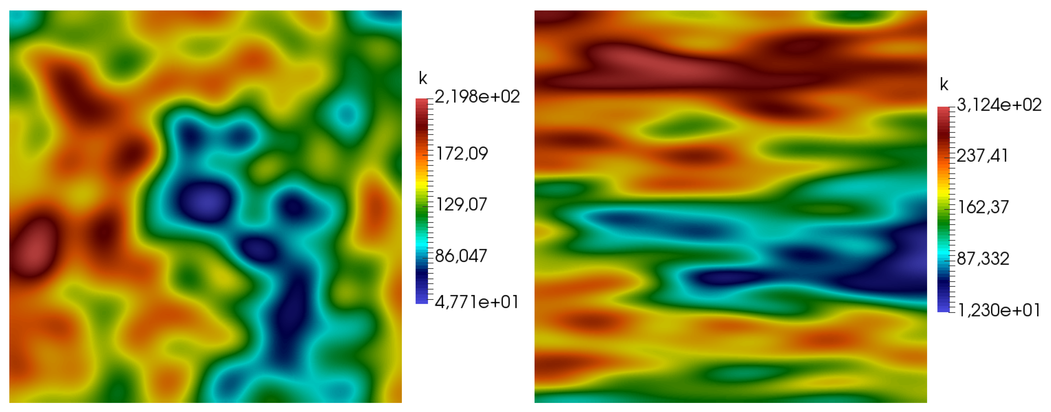
In the numerical study, we set μ = 1 , ρ = 1 , and f = 1 . For the Picard iteration, we set t o l = 10 8 . The permeability tensor k is heterogeneous and presented in Figure 3, where we considered two test cases. We set the Darcy-Forchheimer coefficient β = C · k 1 from [20,21], where the parameter C controls the influence of the nonlinear part of the equation. We studied the proposed multiscale solver for C = 10.24 , C = 34.93 , C = 1584.14 , and C = 71,554.17. With such values of C, we could investigate the behavior of a method with the various influences of the nonlinear part. By increasing the parameter C, we obtained a Darcy-Forchheimer equation with the dominant nonlinear part.
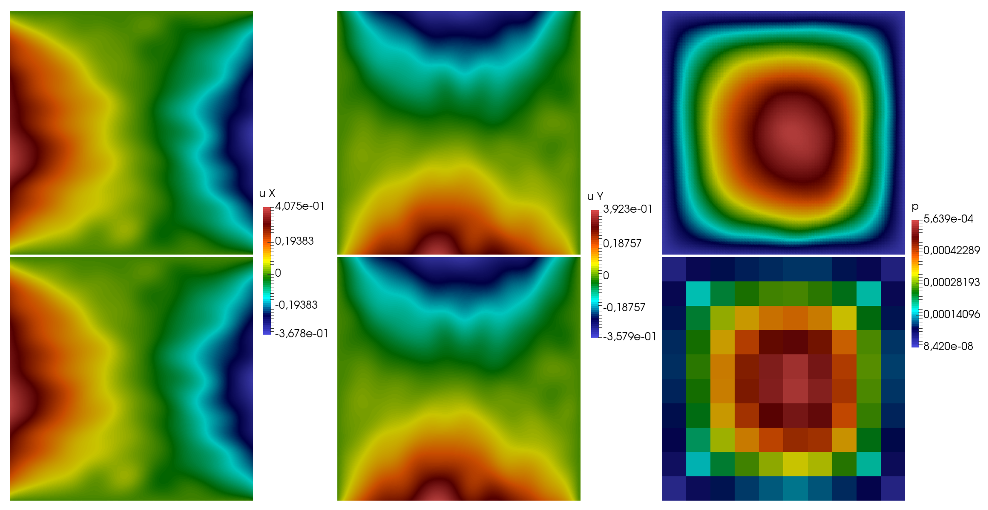
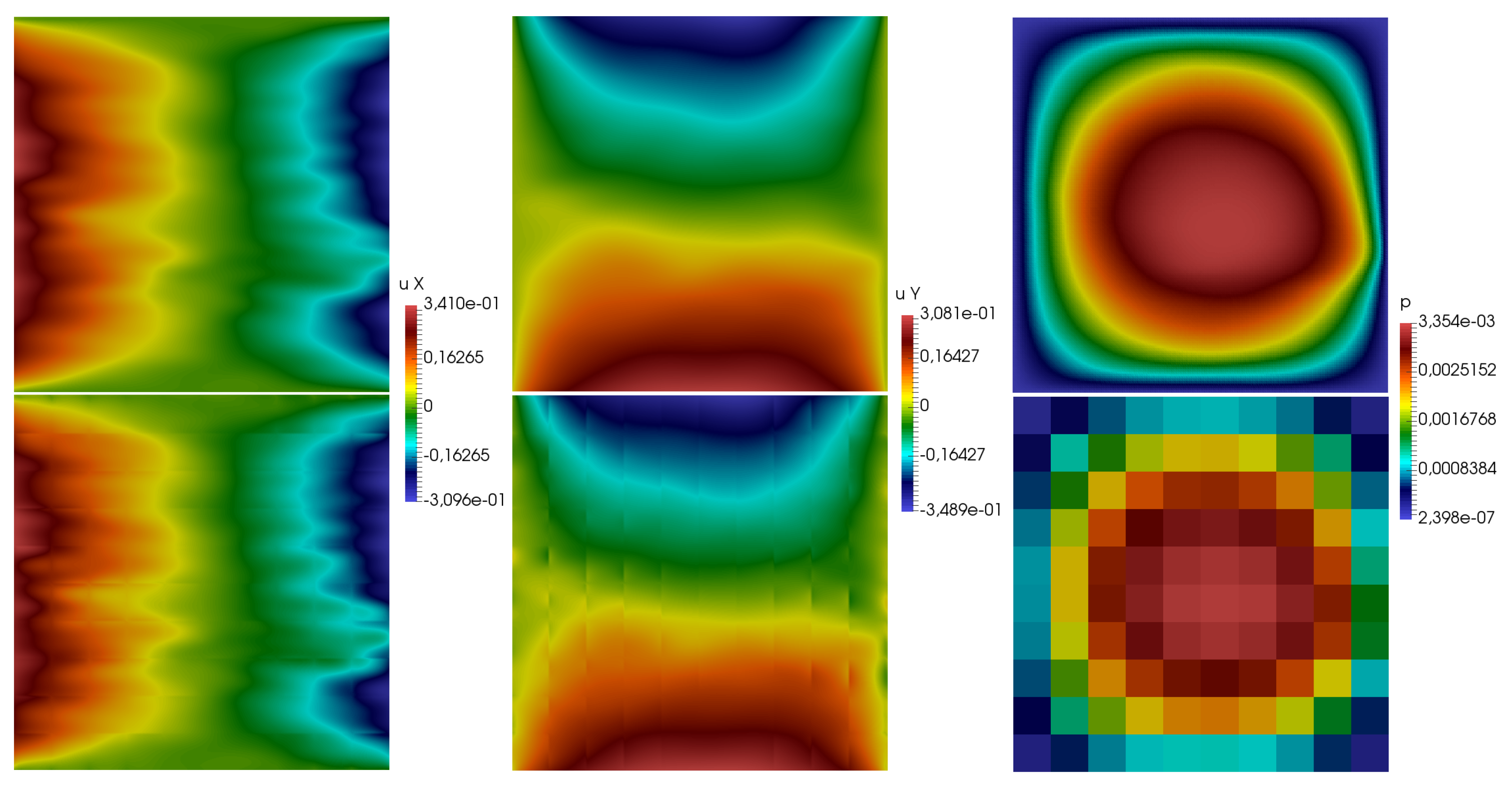
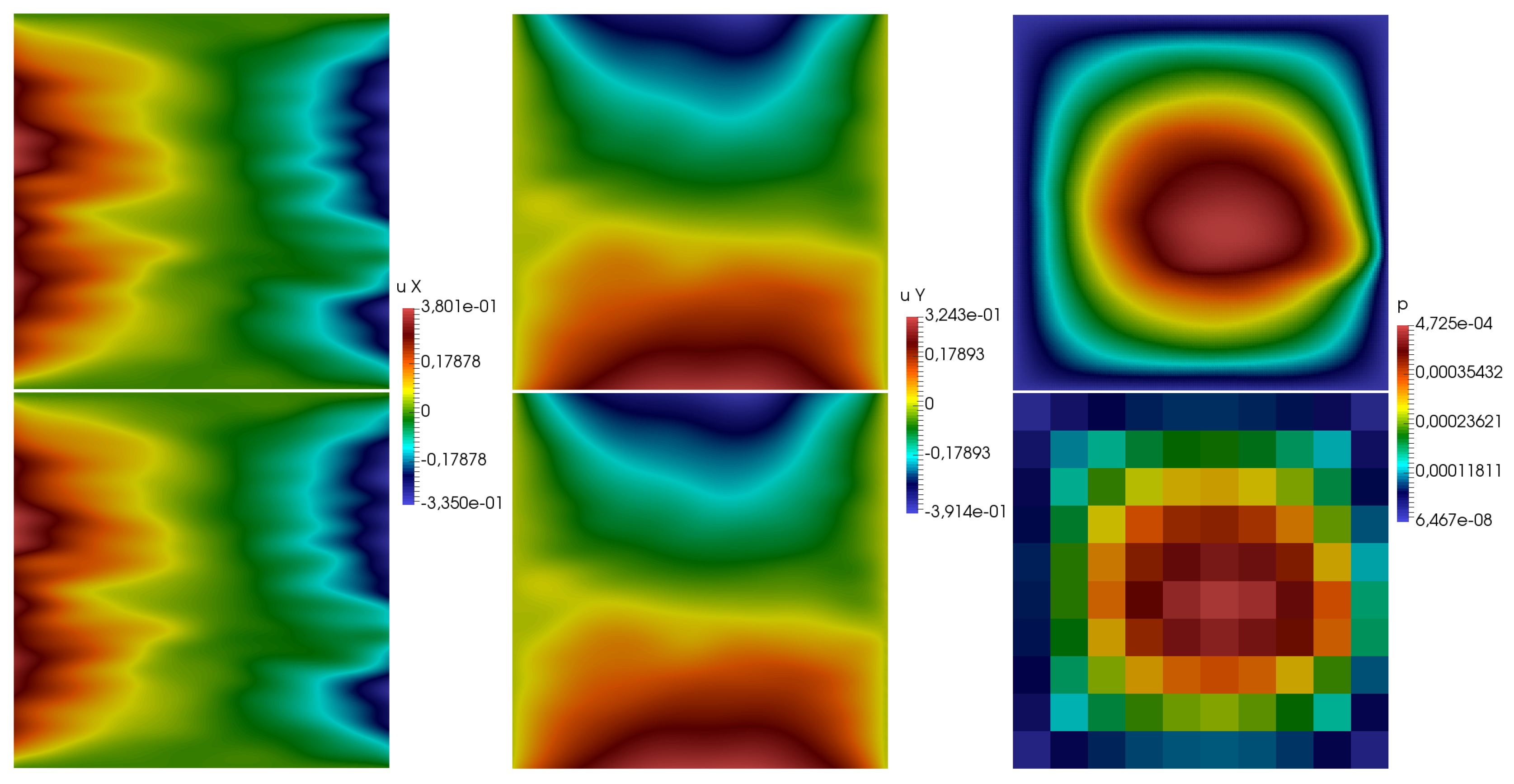
At first, we considered a test case with β = 0 . Fine scale and multiscale solutions using eight multiscale basis functions are presented in Figure 4 and Figure 5 for coefficient k from Test 1 and Test 2. In Table 1, the relative errors in the L 2 norm for different numbers of multiscale basis functions are presented for β = 0 . Here, D O F c and D O F f denote the size of the multiscale and fine grid solutions ( D O F f = 128,320), and M is the number of multiscale basis functions. By #iter, we denote the number of Picard iterations, and e u and e p are the relative errors in L 2 norm for velocity and pressure, respectively. To calculate the error of the pressure, the average values over the coarse grid cells are used.
The numerical results for C = 34.93 with coefficient k from Test 1 and Test 2 using eight multiscale basis functions are presented in Figure 6 and Figure 7. In Table 2, Table 3, Table 4 and Table 5, we show the relative error in the L 2 norm between the multiscale solution and the fine grid solution for different numbers of multiscale basis functions. The errors are presented for different values of C to see the influence of the nonlinear part on the accuracy of mixed GMsFEM. According to the obtained results, we observed that the method worked well with the presented problem. When we increased the number of multiscale bases, we observed that the error decreased. For large values of C the error was greater than for smaller values. This was due to the fact that for large C values, the influence of the nonlinear part of the equation increased, and our multiscale bases did not take into account the nonlinear part. From the tables, we can observe that the number of Picard iterations of mixed GMsFEM was significantly smaller than the number of iterations of the fine grid solution for large C. For Test 1 and Test 2, we obtained similar results for the presented multiscale solver.

6. Conclusions

In this paper, we conducted a numerical study of the solution of the Darcy-Forchheimer model in high contrast heterogeneous media. To solve this problem, we used the mixed multiscale finite element method. The method showed good accuracy in two model problems. The obtained solutions were compared with the fine grid solution using the mixed finite element method. The study showed that the accuracy of this method depended on the number of multiscale basis functions and was almost independent of the influence of the nonlinear part of the equation. Mixed GMsFEM provided a good solution for any β values, and the accuracy of the method was improved by using more basis functions. The method showed good efficiency, since the number of Picard iterations with a large influence of the nonlinear part was much less than when solving a problem on a fine grid.

Author Contributions

The authors have contributed equally to the work.

Funding

D.S.’s and M.V.’s work was supported by the grant of the Russian Scientific Found N17-71-20055 and the mega-grant of the Russian Federation Government (N 14.Y26.31.0013). E.T.C.’s work was partially supported by the Hong Kong RGC General Research Fund (Projects 14304217 and 14302018) and the CUHK Direct Grant for Research 2018-19. The work of J.H. was supported by the China Postdoctoral Science Foundation Funded Project Grant No. BX20180266, 2018M642991, in part by the National Natural Science Foundation of China Grant No. 11901497, and in part by the Natural Science Foundation of Hunan Province Grant No. 2019JJ50607. The work of Y.H. was supported by the National Natural Science Foundation of China Grant No. 11971410 and in part by the Project of Scientific Research Fund of Hunan Provincial Science and Technology Department (2018WK4006).

Conflicts of Interest

The authors declare no conflict of interest.

References

  1. Girault, V.; Wheeler, M.F. Numerical discretization of a Darcy-Forchheimer model. Numer. Math. 2008, 110, 161–198. [Google Scholar] [CrossRef]
  2. Park, E.J. Mixed finite element methods for generalized Forchheimer flow in porous media. Numer. Methods Partial Differ. Equ. 2005, 21, 213–228. [Google Scholar] [CrossRef]
  3. Pan, H.; Rui, H. Mixed element method for two-dimensional Darcy-Forchheimer model. J. Sci. Comput. 2012, 52, 563–587. [Google Scholar] [CrossRef]
  4. Rui, H.; Pan, H. A Block-Centered Finite Difference Method for the Darcy-Forchheimer Model. SIAM J. Numer. Anal. 2012, 50, 2612–2631. [Google Scholar] [CrossRef]
  5. Rui, H.; Zhao, D.; Pan, H. A block-centered finite difference method for Darcy-Forchheimer model with variable Forchheimer number. Numer. Methods Partial Differ. Equ. 2015, 31, 1603–1622. [Google Scholar] [CrossRef]
  6. Rui, H.; Liu, W. A Two-Grid Block-Centered Finite Difference Method For Darcy-Forchheimer Flow in Porous Media. SIAM J. Numer. Anal. 2015, 53, 1941–1962. [Google Scholar] [CrossRef]
  7. Huang, J.; Chen, L.; Rui, H. Multigrid methods for a mixed finite element method of the Darcy-Forchheimer model. J. Sci. Comput. 2018, 74, 396–411. [Google Scholar] [CrossRef] [PubMed]
  8. Chen, Z.; Hou, T. A mixed multiscale finite element method for elliptic problems with oscillating coefficients. Math. Comput. 2003, 72, 541–576. [Google Scholar] [CrossRef] [Green Version]
  9. Aarnes, J.E.; Efendiev, Y.; Jiang, L. Mixed multiscale finite element methods using limited global information. Multiscale Model. Simul. 2008, 7, 655–676. [Google Scholar] [CrossRef]
  10. Aarnes, J.E. On the use of a mixed multiscale finite element method for greaterflexibility and increased speed or improved accuracy in reservoir simulation. Multiscale Model. Simul. 2004, 2, 421–439. [Google Scholar] [CrossRef]
  11. Aarnes, J.E.; Kippe, V.; Lie, K.A. Mixed multiscale finite elements and streamline methods for reservoir simulation of large geomodels. Adv. Water Resour. 2005, 28, 257–271. [Google Scholar] [CrossRef]
  12. Chung, E.T.; Efendiev, Y.; Lee, C. Mixed generalized multiscale finite element methods and applications. Multiscale Model. Simul. 2015, 13, 338–366. [Google Scholar] [CrossRef] [Green Version]
  13. Chung, E.T.; Leung, W.T.; Vasilyeva, M. Mixed GMsFEM for second order elliptic problem in perforated domains. J. Comput. Appl. Math. 2016, 304, 84–99. [Google Scholar] [CrossRef]
  14. Chung, E.T.; Leung, W.; Vasilyeva, M.; Wang, Y. Multiscale model reduction for transport and flow problems in perforated domains. J. Comput. Appl. Math. 2018, 330, 519–535. [Google Scholar] [CrossRef]
  15. Zhang, J.; Xing, H. Numerical modeling of non-Darcy flow in near-well region of a geothermal reservoir. Geothermics 2012, 42, 78–86. [Google Scholar] [CrossRef]
  16. Chang, J.; Nakshatrala, K.B.; Reddy, J.N. Modification to Darcy-Forchheimer model due to pressure-dependent viscosity: Consequences and numerical solutions. J. Porous Media 2017, 20. [Google Scholar] [CrossRef]
  17. Ciarlet, P.G. The Finite Element Method for Elliptic Problems; SIAM: Philadelphia, PA, USA, 2002. [Google Scholar]
  18. Adams, R.; Fournier, J. Sobolev Spaces; Academic Press: New York, NY, USA; London, UK; Toronto, ON, Canada, 1975. [Google Scholar]
  19. Chan, H.Y.; Chung, E.; Efendiev, Y. Adaptive mixed GMsFEM for flows in heterogeneous media. Numer. Math. Theory Methods Appl. 2016, 9, 497–527. [Google Scholar] [CrossRef] [Green Version]
  20. Li, D.; Engler, T.W. Literature review on correlations of the non-Darcy coefficient. In Proceedings of the SPE Permian Basin Oil and Gas Recovery Conference, Midland, TX, YSA, 15–17 May 2001. [Google Scholar]
  21. Muljadi, B.P.; Blunt, M.J.; Raeini, A.Q.; Bijeljic, B. The impact of porous media heterogeneity on non-Darcy flow behaviour from pore-scale simulation. Adv. Water Resour. 2016, 95, 329–340. [Google Scholar] [CrossRef]
Figure 1. Illustration of the heterogeneous property, coarse grid, and multiscale basis functions in the local domain.
Mathematics 07 01212 g001
Figure 2. Coarse grid (left) and fine grid (right).
Mathematics 07 01212 g002
Figure 3. Heterogeneous coefficient for Test 1 (left) and Test 2 (right).
Mathematics 07 01212 g003
Figure 4. Fine grid solution (top) and multiscale solution using eight multiscale basis functions (bottom). Coefficient k from Test 1 with β = 0 .
Mathematics 07 01212 g004
Figure 5. Fine grid solution (top) and multiscale solution using eight multiscale basis functions (bottom). Coefficient k from Test 2 with C = 34.93 .
Mathematics 07 01212 g005
Figure 6. Fine grid solution (top) and multiscale solution using eight multiscale basis functions (bottom). Coefficient k from Test 1 with C = 34.93 .
Mathematics 07 01212 g006
Figure 7. Fine grid solution (top) and multiscale solution using eight multiscale basis functions (bottom). Coefficient k from Test 2 with β = 0 .
Mathematics 07 01212 g007
Table 1. Relative error in the L 2 norm for different numbers of multiscale basis functions. Coefficient k from Test 1 (left) and Test 2 (right) with β = 0 .
M DOF c e u , % e p , %M DOF c e u , % e p , %
132010.0691.212132011.2791.451
25401.1120.03125402.9430.104
49800.2530.00149800.5790.004
818600.0610.001818600.1520.001
Table 2. Relative error in the L 2 norm for different numbers of multiscale basis functions. Coefficient k from Test 1 (left) and Test 2 (right) with C = 10.24 .
M DOF c e u , % e p , %#iterM DOF c e u , % e p , %#iter
132010.3341.8569132011.0422.1557
25402.3290.136825403.5850.2526
49802.1740.129749802.8970.1995
818602.0540.1026818602.8560.1955
Iterations on the fine grid = 5Iterations on the fine grid = 5
Table 3. Relative error in the L 2 norm for different numbers of multiscale basis functions. Coefficient k from Test 1 (left) and Test 2 (right) with C = 34.93 .
M DOF c e u , % e p , %#iterM DOF c e u , % e p , %#iter
132010.3892.05224132011.0212.37422
25402.7660.1712325404.0590.31920
49802.5670.1512149803.4690.24819
818602.5610.15119818603.4460.24417
Iterations on the fine grid = 21Iterations on the fine grid = 21
Table 4. Relative error in the L 2 norm for different numbers of multiscale basis functions. Coefficient k from Test 1 (left) and Test 2 (right) with C = 1581.14 .
M DOF c e u , % e p , %#iterM DOF c e u , % e p , %#iter
132010.4152.181387132011.0332.518399
25402.9980.19740325404.3640.364388
49802.8140.17738949803.8680.294371
818602.7990.175368818603.8430.291348
Iterations on the fine grid = 1162Iterations on the fine grid = 1143
Table 5. Relative error in the L 2 norm for different numbers of multiscale basis functions. Coefficient k from Test 1 (left) and Test 2 (right) with C = 71,554.17.
M DOF c e u , % e p , %#iterM DOF c e u , % e p , %#iter
132010.4162.185744132011.0332.522794
25403.0030.19885425404.3720.365809
49802.8210.17788649803.8780.295805
818602.8050.176864818603.8530.291777
Iterations on the fine grid = 16,489Iterations on the fine grid = 14,466

