On Multilevel and Control Variate Monte Carlo Methods for Option Pricing under the Rough Heston Model

Abstract

The rough Heston model is a form of a stochastic Volterra equation, which was proposed to model stock price volatility. It captures some important qualities that can be observed in the financial market—highly endogenous, statistical arbitrages prevention, liquidity asymmetry, and metaorders. Unlike stochastic differential equation, the stochastic Volterra equation is extremely computationally expensive to simulate. In other words, it is difficult to compute option prices under the rough Heston model by conventional Monte Carlo simulation. In this paper, we prove that Euler’s discretization method for the stochastic Volterra equation with non-Lipschitz diffusion coefficient $\mathbb{E}\left[\right|V_t-V_t^n{|}^p]$ is finitely bounded by an exponential function of t. Furthermore, the weak error $\left|\mathbb{E}\right[V_t-V_t^n\left]\right|$ and convergence for the stochastic Volterra equation are proven at the rate of $\mathcal{O}\left(n^{-H}\right)$. In addition, we propose a mixed Monte Carlo method, using the control variate and multilevel methods. The numerical experiments indicate that the proposed method is capable of achieving a substantial cost-adjusted variance reduction up to 17 times, and it is better than its predecessor individual methods in terms of cost-adjusted performance. Due to the cost-adjusted basis for our numerical experiment, the result also indicates a high possibility of potential use in practice.

1. Introduction

Rough volatility has recently emerged as an impressive tool to model an asset’s volatility in the financial market. The empirical study [1] by Gatheral and his co-authors have made all this possible. In short, rough volatility is a type of fractional Brownian motion (fBm) with a Hurst parameter of $0<H<0.5$, or in terms of alpha notation, $0.5<\alpha =H+0.5<1$. Specifically, fBm with $0<H<0.5$ has rougher fluctuation than the ordinary Brownian motion, whereas fBm with $0.5<H<1$ has a smaller/lesser fluctuation than the ordinary Brownian motion. Before continuing the discussion on rough volatility, we would like to mention some of the work that made this discovery possible. First, before the introduction of rough volatility, the fractional Brownian motion with $0.5<H<1$ was used to model the long-term memory effect in the asset’s volatility by Comte and Renault [2]. Subsequently, mixed fractional Brownian motion, composing the sum of fractional Brownian motion and ordinary Brownian motion, was proposed to also model the volatility of the asset return in the work by Cheridito et al. [3].

One of the earliest work that uses fractional Brownian motion with $0<H<0.5$ as a volatility component in option pricing is by Alos et al. [4]. In particular, the authors managed to generate a short-time-to-maturity at-the-money-term-structure skew of the order $\mathcal{O}\left(T^c\right)$ for $c>-0.5$. This is a great accomplishment, as the individual local and stochastic volatility models are unable to replicate the mentioned behavior previously. Fukasawa [5] also demonstrated that option prices with volatility driven by the stochastic volatility model with the fractional Brownian motion of the Hurst parameter $0<H<0.5$ can generate an at-the-money volatility skew of the order $\mathcal{O}\left(T^{H-0.5}\right)$.

Due to recent advancements in rough volatility, there are many studies revolving around the development of rough volatility models. In particular, the authors of [6] proposed the rough Bergomi (rBergomi) model, which is a rough extension of the Bergomi model [7]. The result of the study found that the rBergomi model with fewer parameters fits the SPX volatility relatively better than Markovian stochastic volatility models; this is consistent with the SPX variance swap during the year 2008 economic crisis and the flash crash event. The rough Heston model is the main discussion of this paper and it was proposed by El Euch et al. in the work of [8,9]. What is so special about the rough Heston model is that it can fit the implied volatility of the options very well, and it can replicate the explosive behavior of the term-structure at-the-money skew observed in the financial market. Several studies [10,11,12,13,14,15] mainly focus on computational reduction of the rough Heston model. One of the greatest barriers to compute option prices under the rough Heston model is due to the lack of an explicit solution for the fractional Riccati equation, which is a part of the characteristic function of the option prices under the rough Heston model.

This paper contributes in three ways: (1) presents and proves a time bound on Euler’s discretization method for the simulation of the stochastic Volterra equation $\mathbb{E}\left[\right|V_t-V_t^n{|}^p]$ with a non-Lipschitz diffusion coefficient; (2) proves the weak error rate $\left|\mathbb{E}\right[V_t-V_t^n\left]\right|$ and weak convergence of Euler’s discretization method on the same stochastic Volterra equation; and (3) proposes a control variate estimator and a mixed Monte Carlo method to enhance the computational efficiency in computing the option price under the rough Heston model. Our work is possible mainly due to the work of [16,17,18,19,20,21]. The following Section 1.1 provides a simple and short introduction to our work. Section 2 mainly talks about discretization methods—the Euler–Maruyama (first-order Euler) method for the stochastic differential equation and stochastic Volterra equation, as well as the second-order Euler method for the stochastic differential equation. The bounded and weak errors of the Euler discretization method are also presented; the proofs are located in Appendix A, Appendix B and Appendix C. Furthermore, we discuss some existing Monte Carlo methods (base, control variate, and multilevel) and propose a mixed Monte Carlo (multilevel control variate) method in Section 3. Section 4 is dedicated to the numerical experiment of some existing methods and the proposed method. Specifically, we consider a few of the tests to benchmark our methods: (1) the capability of implied volatility to change on parameters $\rho ,\alpha$, and T; (2) cost-adjusted variation comparisons for OTM, ATM, and ITM options as well as the comparisons for different estimators; the (3) discretization bias for different estimators on a different number of time steps n and level L.

1.1. Prerequisites

The rough Heston model can be formulated as follows:

$$\frac{d{S}_t}{S_t}={\sigma }_t\left[\rho d{W}_t^1+\sqrt{1-{\rho }^2}d{W}_t^2\right]$$

(1)

and

$${\sigma }_t^2={\sigma }_0^2+\frac{1}{\Gamma \left(\alpha \right)}{\int }_0^t{(t-s)}^{\alpha -1}\lambda [\theta -{\sigma }_s^2]ds+\frac{\nu }{\Gamma \left(\alpha \right)}{\int }_0^t{(t-s)}^{\alpha -1}{\sigma }_{s}d{W}_s^1,$$

(2)

where S is the stock price, $\rho$ is the correlation between $d{W}_t^1$ and $d{W}_t^2$, $0.5<\alpha <1$ is the parameter to control the roughness of the volatility movements, $\theta$ is the mean reversion level for the variance of return, $\lambda >0$ is the speed at which the variance is reverting to its mean reversion level, $\nu >0$ is the magnitude of random movement of the variance of the return.

Proposition 1.

Assume the rough Heston model in Equation (2), and then the conditional expectation of the variance is as follows:

$${\mathbb{E}}_0\left[{\sigma }_t^2\right]={\sigma }_0^2+(\theta -{\sigma }_0^2){\int }_0^t{f}^{\alpha ,\lambda }\left(s\right)ds,$$

(3)

where

$$f^{\alpha ,\lambda }\left(t\right)=\lambda t^{\alpha -1}{E}_{\alpha ,\alpha }(-\lambda t^{\alpha }),$$

(4)

such that$E_{\alpha ,\beta }\left(x\right)={\sum }_{n=0}^{\infty }\frac{x^n}{\Gamma (\alpha n+\beta )}$denotes the generalized Mittag–Leffler function.

Proof. 

It was proven in several studies—Proposition 3.1 [22], Proposition 2.1 [23], and page 7–8 of [24]. □

2. Discretization Methods

This section mainly discusses the first-order Euler discretization method for the stochastic differential equation and stochastic Volterra equation, and together with the second-order Euler discretization methods for the stochastic differential equation.

2.1. Euler–Maruyama Discretization Method

We first consider the stock process S satisfying the following stochastic differential equation (SDE):

$$d{S}_t=a\left(S_t\right)dt+b\left(S_t\right)d{W}_t,$$

(5)

where $a,b:\mathbb{R}\to \mathbb{R}$ are coefficient functions, and W is an independent standard Brownian motion. Specifically, the coefficient functions a and b are assumed to satisfy the usual conditions (see Appendix B.2 in [18]) for the existence and uniqueness of a strong solution to the SDE (5). The initial condition of SDE (5) is set as $S\left(0\right)$.

First off, we denote the time-discretized approximation of the process S as $\widehat{S}$. Under the Euler–Maruyama method [25], the initial condition remains the same as ${\widehat{S}}_0=S_0$, and the SDE (5) is discretized on a time grid $0=t_0<t_1<\dots <t_m$ as follows:

$${\widehat{S}}_{t_{i+1}}={\widehat{S}}_{t_i}+a({\widehat{S}}_{t_i})[t_{i+1}-t_i]+b({\widehat{S}}_{t_i})\sqrt{t_{i+1}-t_i}{Z}_{i+1},$$

(6)

where $i=0,\dots ,m-1$, and Z is an independent standard Brownian motion $Z\sim N(0,1)$. In this work, we limit the method’s time grid to linear fixed spacing such that $t_i=i\delta$, where $\delta$ is the fixed space. It is widely known that the Euler–Maruyama method for SDE has a strong error of $\mathcal{O}\left(\sqrt{\delta }\right)$. Furthermore, it can be easily further refined to $\mathcal{O}\left(\delta \right)$, using Itô’s formula to expand $b\left(S\right(t\left)\right)$ [26] instead, but we will avoid further discussing this method, as we will introduce the second-order Euler method or Milstein scheme later. See Chapter 6 in [18] for more details.

Suppose now we consider the stochastic Volterra equation (SVE) of the following form:

$$V_t=V_0+{\int }_0^t{K}_1(t,s)m(s,V_s)ds+{\int }_0^t{K}_2(t,s)g(s,V_s)d{W}_s,t\in [0,T],$$

(7)

where $m,g:[0,T]\times \mathbb{R}\to \mathbb{R}$ and $K_1,K_2$ are the (possibly singular) kernels. We refer to the work of [21] on the discussion of discrete-time simulation of SVE for the Lipschitz condition. Notably, we can outline the following modified assumptions (one-dimensional space) stated in page 3 of [21] in order to provide theorems on the error of Euler’s discretization method for SVE related to the rough Heston model (non-Lipschitz diffusion coefficient).

Assumption 1.

We first denote the fixed space as $\delta :=\Delta t_{i+1}=t_{i+1}-t_i\le 1$, then let $n\ge 1$ such that $t_n=T$. Furthermore, we denote $\eta \left(s\right):=t_i$ for $s\in [t_i,t_{i+1})$ for $i\ge 0$ and again denote the following fixed constants $\beta \in (1,1/(1-2H\left)\right),H\in (0,1/2),\kappa \in (0,1),C>0$.

(AA1)

For $i=1,2$, let $K_i(t,u)=0$ when $u\ge t$, and the following holds:

$${\int }_0^t\left(K_i{(t,u)}^2+K_i{(t,u)}^{2\beta }+K_i{(t,\eta \left(u\right))}^2+K_i{(t,\eta \left(u\right))}^{2\beta }\right)du<\infty$$

(8)

for all $t\in [0,T]$.

(AA2)

For $i=1,2$, and $s\le t$, the following holds:

$${\int }_s^t{K}_i{(t,u)}^{2}ds+{\int }_s^t{K}_i{(t,\eta \left(u\right))}^{2}ds\le C{(t-s)}^{2H}.$$

(9)

(AA3)

For $i=1,2$, and $s\le t$, the following holds:

$${\int }_s^t{K}_i{(t,u)}^{2\beta }ds+{\int }_s^t{K}_i{(t,\eta \left(u\right))}^{2\beta }ds\le C{(t-s)}^{(2H-1)\beta +1}.$$

(10)

(AA4)

For $i=1,2$, the following holds:

$${\int }_0^t{[K_i(t+\delta ,u)-K_i(t,u)]}^{2}ds+{\int }_0^t{[K_i(t+\delta ,\eta \left(u\right))-K_i(t,\eta \left(u\right))]}^{2}du\le C{\delta }^{2H}.$$

(11)

(AA5)

For $i=1,2$, the following holds:

$${\int }_0^t{[K_i(t+\delta ,u)-K_i(t,u)]}^{2\beta }du\le C{\delta }^{(2H-1)\beta +1}.$$

(12)

(AA6)

For $i=1,2$, the following holds:

$${\int }_0^t{[K_i(t,u)-K_i(t,\eta \left(u\right))]}^{2}ds\le C{\delta }^{2H}.$$

(13)

(AA7)

For $i=1,2$, the following holds:

$${\int }_0^t{[K_i(t,u)-K_i(t,n\left(u\right))]}^{2\beta }du\le C{\delta }^{(2H-1)\beta +1}.$$

(14)

(BB1)

For $x,y\in \mathbb{R}$ and $s,t\in [0,T]$, let $\left|\right(m,g\left)\right(0,0\left)\right|\le C$ hold. The following inequalities hold:

$$\begin{array}{cc}\hfill \left|m\right(t,x)-m(t,y\left)\right|& \le C|x-y|,\hfill \end{array}$$

(15)

$$\begin{array}{cc}\hfill \left|g\right(t,x)-g(t,y\left)\right|& \le {C|x-y|}^{\kappa },\hfill \end{array}$$

(16)

$$\begin{array}{cc}\hfill \left|\right(m,g\left)\right(t,x\left)\right|& \le C(1+|x\left|\right),\hfill \end{array}$$

(17)

$$\begin{array}{cc}\hfill \left|\right(m,g\left)\right(t,x)-(m,g\left)\right(s,x\left)\right|& \le {C|t-s|}^H(1+|x\left|\right).\hfill \end{array}$$

(18)

Lemma 1.

Suppose that we let $K_i(t,u)={(t-u)}^{H-1/2}$ for $i=1,2$; then, it satisfies conditions (AA1)–(AA7).

Proof. 

See Appendix A. □

The SVE in the first-order Euler discretized form is as follows:

$$\begin{array}{cc}\hfill V_{t_{i+1}}^n=& V_{t_i}^n+\sum _{k=0}^{i-1}\left(K_1(t_{i+1},t_k)-K_1(t_i,t_k)\right)m(t_k,V_{t_k}^n)\Delta t_{k+1}+K_1(t_{i+1},t_i)m(t_i,V_{t_i}^n)\Delta t_{i+1}\hfill \\ \hfill & +\sum _{k=0}^{i-1}\left(K_2(t_{i+1},t_k)-K_2(t_i,t_k)\right)g(t_k,X_{t_k}^n)\Delta W_{k+1}+K_2(t_{i+1},t_i)g(t_i,V_{t_i}^n)\Delta W_{i+1},\hfill \end{array}$$

(19)

where $\Delta t_{i+1}=t_{i+1}-t_i=\delta$ and $\Delta W_{i+1}=W_{t_{i+1}}-W_{t_i}$ for $i=0,1,\dots ,n-1$. Note that we use the following solution $V_t^n$ of the Euler scheme (integral form) in the bounded proof of the Euler discretization method.

$$V_t^n=V_0+{\int }_0^t{K}_1(t,\eta \left(u\right))m(\eta \left(u\right),V_{\eta \left(u\right)}^n)du+{\int }_0^t{K}_2(t,\eta \left(u\right))g(\eta \left(u\right),V_{\eta \left(u\right)}^n)d{W}_u.$$

(20)

Theorem 1.

Suppose that Assumption 1, conditions (AA1)–(AA7) and condition (BB1) hold. Let $p\ge {\displaystyle \frac{2\beta }{\kappa (\beta -1)}}$ for $\beta \in (1,1/(1-2H\left)\right)$ and $\kappa \in (0,1)$; then, there exists a finite constant $C>0$ that depends on $T,p,V_0$, and β such that for $t\in [0,T]$ and $n\to \infty$, the following is true:

$$\underset{n\to \infty }{lim}\mathbb{E}\left[\right|V_t-V_t^n{|}^p]\le {\left[C(exp(Ct)-1)\right]}^{1/(1-\kappa )}.$$

(21)

Proof. 

Take the limit $n\to \infty$ in Theorem A1, and note that $ϵ>0$; then, the result follows directly. See Appendix B □

Remark 1.

We note that the Assumptions 1, conditions (AA1)–(AA7) and condition (BB1) satisfy the case of the rough Heston model. In addition, in the case of the rough Heston model, we have the non-Lipschitz diffusion coefficient factor of $\kappa =1/2$. Finally, it can be seen that for small time t, the bounded errors are small too. On the other note, we do have to mention that in the case of the Lipschitz condition for the diffusion coefficient in the stochastic Volterra equation, i.e., $\left|g\right(t,x)-g(t,y\left)\right|\le C|x-y|$, ${lim}_{n\to \infty }\mathbb{E}\left[\right|V_t-V_t^n{|}^p]=0$ as proven in [21].

Theorem 2.

Suppose that Assumption 1, conditions (AA1)–(AA7) and condition (BB1) hold. Then, the following is true:

$$\underset{n\to \infty }{lim}|\mathbb{E}\left[V_t\right]-\mathbb{E}\left[V_t^n\right]|=0.$$

(22)

Proof. 

Take the limit $n\to \infty$ in Theorem A2, then the result follows immediately. See Appendix C. □

Remark 2.

Theorem 2 shows the weak convergence of the variance process in the rough Heston model. This was actually proven in [27], but here, we provide the weak error order for the variance process of the rough Heston model. From Theorem 2, we know that the variance process converges at the rate of ${\delta }^{(1/2\beta )\left[\right(2H-1)\beta +1]}$, where $\delta =T/n$ and $\beta \in (1,1/(1-2H\left)\right)$. Since β can be specifically picked, our goal is to maximize the convergence order $(1/2\beta )\left[\right(2H-1)\beta +1]$ by changing β. We differentiate the order with respect to β as follows:

$$\frac{\partial }{\partial \beta }\left[\frac{1}{2\beta }\left((2H-1)\beta +1\right)\right]=-\frac{1}{2{\beta }^2}.$$

(23)

From Equation (23), we know that $(1/2\beta )\left[\right(2H-1)\beta +1]$ is strictly decreasing on the range of $\beta \in (1,1/(1-2H\left)\right)$. Then, the weak error order can be obtained as follows:

$$\underset{\beta \to 1}{lim}\frac{1}{2\beta }\left((2H-1)\beta +1\right)=H.$$

(24)

This indicates that the weak error of the rough Heston model is $O\left(n^{-H}\right)$.

2.2. Second-Order Euler Discretization Method

In this subsection, we discuss the second-order Euler discretization method that was introduced by Milstein [28] (we refer to the text [18]). Let us consider the stock process (5) in another manner, i.e., the following:

$$S_{t+\delta }=S_t+{\int }_t^{t+\delta }a(u,S_u)du+{\int }_t^{t+\delta }b(u,S_u)d{W}_u.$$

(25)

We denote the following operators:

$${\mathcal{L}}^0=\frac{\partial }{\partial t}+a\frac{\partial }{\partial s}+\frac{1}{2}{b}^2\frac{{\partial }^2}{\partial s^2}$$

(26)

and

$${\mathcal{L}}^1=b\frac{\partial }{\partial s}.$$

(27)

Then, the terms ${\int }_t^{t+\delta }a\left(S\left(u\right)\right)du$ and ${\int }_t^{t+\delta }b\left(S\left(u\right)\right)d{W}_u$ can be approximated as follows:

$${\int }_t^{t+\delta }a(u,S\left(u\right))du\approx a(t,S_t)\delta +{\mathcal{L}}^{0}a(t,S_t)I_1+{\mathcal{L}}^{1}a(t,S_t)I_2$$

(28)

and

$${\int }_t^{t+\delta }b(u,S\left(u\right))d{W}_u\approx b(t,S_t)[W(t+\delta )-W\left(t\right)]+{\mathcal{L}}^{0}b(t,S_t)I_3+{\mathcal{L}}^{1}b(t,S_t)I_4,$$

(29)

where $I_i$ for $i=1,\dots ,4$ denotes the double integral, which can be computed as follows:

$$\begin{array}{}(30)& \hfill I_1& =\frac{1}{2}{\delta }^2,\hfill (31)& \hfill I_3& =\delta \Delta W-I_2,\hfill (32)& \hfill I_4& =\frac{1}{2}[{(\Delta W)}^2-\delta ],\hfill \end{array}$$

where $\Delta W=W_{t+\delta }-W_t$. The computation of $I_2$ requires some derivation. Based on Chapter 6.2 in [18], $I_2$ can be simulated as follows:

$$\left(\begin{array}{c}\Delta W\\ I_2\end{array}\right)\sim N\left(\begin{array}{c}0,\left(\begin{array}{cc}\delta & \frac{1}{2}{\delta }^2\\ \frac{1}{2}{\delta }^2& \frac{1}{3}{\delta }^3\end{array}\right)\end{array}\right),$$

(33)

The correlation between $\Delta W$ and $I_2$ can be computed as follows:

$$\begin{array}{}(34)& \hfill {\rho }_{\Delta W,I_2}& =\frac{Cov(\Delta W,I_2)}{\sqrt{Var(\Delta W)Var\left(I_2\right)}}\hfill (35)& & =\frac{\frac{1}{2}{\delta }^2}{\sqrt{\delta }\sqrt{\frac{1}{3}{\delta }^3}}=\frac{\sqrt{3}}{2}.\hfill \end{array}$$

Then, we let B denote an independent Brownian motion and $\Delta B\sim N(0,1)$. Finally, we can obtain the following:

$$\begin{array}{}(36)& \hfill I_2& =\sqrt{\frac{1}{3}{\delta }^3}\left[{\rho }_{\Delta W,I_2}\sqrt{\frac{1}{\delta }}\Delta W+\sqrt{1-{\rho }_{\Delta W,I_2}^2}\Delta B\right]\hfill (37)& & =\sqrt{\frac{1}{3}{\delta }^3}\left[\frac{\sqrt{3}}{2}\sqrt{\frac{1}{\delta }}\Delta W+\sqrt{1-\frac{3}{4}}\Delta B\right]\hfill (38)& & =\frac{1}{2}\delta \Delta W+\frac{1}{2\sqrt{3}}{\delta }^{3/2}\Delta B.\hfill \end{array}$$

See [18] for specific details of the derivation of Equations (30)–(33). It was shown by [29] that the second-order Euler discretization method has a weak order of error of $\mathcal{O}\left({\delta }^2\right)$; it has a better convergence order than the first-order Euler discretization method, which possesses a weak error of $\mathcal{O}\left(\delta \right)$. However, the requirement that comes with the weak order of convergence on the second-order Euler discretization method requires the evaluated functions a and b to have uniformly bounded derivatives, and the functions need to be six times continuously differentiable. The purpose of giving a short review on this method is because while we will not be using this method for the discretization of the stochastic Volterra equation, we can actually use this on the discretization of the stock process in the control variate method and multilevel control variate method (control variate part) instead of the first-order Euler discretization method. We can reduce the overall error of the simulation in numerical experiment as per the weak error that the second-order Euler discretization method has suggested.

3. Monte Carlo Methods

This section outlines the conventional Monte Carlo method, control variate method, multilevel Monte Carlo methiod, and the novel multilevel control variate Monte Carlo method.

Suppose that the interest of our study is to estimate the $\mathbb{E}\left[P\right]$, the conventional Monte Carlo method estimates $\mathbb{E}\left[P\right]$, using N independent samples of $\omega$ with a given probability space $(\Omega ,\mathcal{F},\mathbb{P})$, that is, the following:

$$\widehat{P}=\frac{1}{N}\sum _{n=1}^{N}P({\omega }^{\left(n\right)}).$$

(39)

The variance of this estimator is $\frac{1}{N}Var\left[P\right]$, and the root mean square error (RMS) of the estimator has an order of $\mathcal{O}\left(N^{-1/2}\right)$. Particularly, suppose that we require an accuracy of $ϵ$ for the RMS for the estimator; then, a total of $N=\mathcal{O}\left({ϵ}^{-2}\right)$ samples are needed for the conventional Monte Carlo.

3.1. Control Variate Method

The control variate method is one of the variance reduction methods along with antithetic variates, quasi Monte Carlo, and importance sampling methods. The idea of the control variate method is somewhat simple. Suppose we consider another random variable X that is paired with P such that the pairs $(X_n,P_n)$ for $n=1,\dots ,N$ are simulated with the sample path $\omega$. Furthermore, it is required that $\mathbb{E}\left[X\right]$ is known, or it can be computed relatively cheaply and accurately. Then, we denote a fixed constant $\varsigma$ such that we can compute the following:

$$P_n\left(\varsigma \right)=P_n-\varsigma (X_n-\mathbb{E}\left[X\right]).$$

(40)

Equation (40) is a control variate estimator, and it is an unbiased estimator to P as follows:

$$\begin{array}{cc}\hfill \underset{N\to \infty }{lim}\frac{1}{N}\sum _{n=1}^N{P}_n\left(\varsigma \right)& =\underset{N\to \infty }{lim}\frac{1}{N}\sum _{n=1}^N\left[P_n-\varsigma (X_n-\mathbb{E}\left[X\right])\right]\hfill \\ & =\mathbb{E}\left[P\right].\hfill \end{array}$$

To optimally reduce the variance or mean square error of the estimator (40), we can pick the constant $\varsigma$ to be the following:

$${\varsigma }^{*}=\frac{{\sigma }_P}{{\sigma }_X}{\rho }_{X,P}=\frac{Cov(X,P)}{Var\left(X\right)}.$$

(41)

The ratio of the control variate estimator to the base estimator is as follows:

$$\frac{Var[P-\varsigma (X-\mathbb{E}\left[X\right]\left)\right]}{Var\left[P\right]}=1-{\rho }_{X,P}^2.$$

(42)

Equation (42) tells us that as long as the correlation between the random variable X and P is negatively correlated or positively correlated, variance reduction is guaranteed. Since the quantity of interest P is usually lacking $\mathbb{E}\left[P\right]$ in practice, we ought to use the optimal sample estimate of $\varsigma$ from Equation (41) as follows:

$${\widehat{\varsigma }}^{*}=\frac{{\sum }_{n=1}^N(X_n-\overline{X})(P_n-\overline{P})}{{\sum }_{n=1}^N{(X_n-\overline{X})}^2},$$

(43)

where $\overline{X}$ and $\overline{P}$ are the sample mean of $X_n$ and $P_n$, respectively. Accordingly, the expectation $\mathbb{E}\left[P\right]$ can be estimated using the sample mean estimator $\overline{P}\left({\widehat{\varsigma }}^{*}\right)$ such that the optimally variance reduced control variate estimator is as follows:

$$P^{CV}=\frac{1}{N}\sum _{n=1}^N\left[P_n-{\widehat{\varsigma }}^{*}(X_n-\overline{X})\right].$$

(44)

In practice, ${\widehat{\varsigma }}^{*}$ and $\overline{X}$ are most likely unknown variables, so it should be estimated beforehand. Pre-running a small number of samples is usually the only way to estimate ${\widehat{\varsigma }}^{*}$ and $\overline{X}$ since this study focuses on call option pricing under the rough Heston model. Obviously, $P={(S_T-K)}^{+}$ is the payoff of the call option prices where $S_T$ is the stock price at maturity time and K is the strike price. Now comes the question of what control variate we should employ in order to get ${\rho }_{X,P}$ to be closest to 1 or $-1$. We propose a control variate based on the idea of [19].

Proposition 2.

Let $S_0^{CV}$ be the initial stock price and W be an independent Brownian motion. Consider the stock process as follows:

$$d{S}_t^{CV}=\sigma \left(t\right)S_t^{CV}d{W}_t,$$

(45)

where $\sigma \left(t\right)$ is a nonrandom function of t. Then, there is an analytic solution for the European call option as follows:

$$\begin{array}{cc}\hfill C& =\mathbb{E}\left[{(S_T^{CV}-K)}^{+}\right]\hfill \\ & =S_0^{CV}N\left(d_{+}\right)-KN\left(d_{-}\right),\hfill \end{array}$$

where $N(·)$ denotes the cumulative distribution function of the standard normal distribution and

$$d_{\pm }=\frac{log{\displaystyle \frac{S_0^{CV}}{K}}\pm {\displaystyle \frac{1}{2}}\overline{\sigma }{}_T^{2}T}{\overline{\sigma }{}_T\sqrt{T}}$$

(46)

such that $\overline{\sigma }{}_T^2=\frac{1}{T}{\int }_0^T{\sigma }^2\left(t\right)dt$.

Proof. 

See page 253 of [30]. □

We propose a control variate X by using Proposition 1. We start by denoting

$$X_T={(S_T^{CV}-K)}^{+},$$

(47)

where $S_t^{CV}$ is the stock process governed by the following:

$$d{S}_t^{CV}=\sigma \left(t\right)S_t^{CV}d{W}_t.$$

(48)

Specifically, $\sigma \left(t\right)$ is a nonrandom function and the squared-function is denoted as follows:

$${\sigma }^2\left(t\right)={\mathbb{E}}_0\left({\sigma }_{t+\epsilon }^2\right),$$

(49)

where ${\mathbb{E}}_0\left({\sigma }_t^2\right)$ is the expectation from Proposition 1, and $\epsilon >0$ is a small positive constant. The use of $t+\epsilon$ in Equation (49) is to ensure that the conditions and requirements of the second-order Euler discretization method are being met. We set $\epsilon =\delta /10$ for our study to avoid the singularity at $\sqrt{{\mathbb{E}}_0^{\prime }\left({\sigma }_t^2\right)}{|}_{t=0}$, where $\delta$ is the step-size of the discretization method. Hence, the expectation of the call option price can be determined using Proposition 2. In a numerical experiment, the forward variance of the rough Heston model (Equation (3)) in Proposition 1 is computed through the truncated Mittag–Leffler function and numerical integration.

3.2. Multilevel Monte Carlo

Multilevel Monte Carlo is a form of the control variate method which uses multiple controls. Specifically, it uses itself with different level of coarseness as control variates. Instead of simulating the process at the finest level, the method approximates $P_L$, using the sequence of $P_0,\dots ,P_{L-1}$. In particular, the sequence $P_0,\dots ,P_{L-1},P_L$ is a sequence with increasing cost to simulate. The expectation of $\mathbb{E}\left[P_L\right]$ can be decomposed as follows:

$$\mathbb{E}\left[P_L\right]=\mathbb{E}\left[P_0\right]+\sum _{i=1}^L\mathbb{E}[P_i-P_{i-1}].$$

(50)

Consequently, we can rely on the following unbiased estimator of $\mathbb{E}\left[P_L\right]$ in practice:

$$P^{ML}=\frac{1}{N_0}\sum _{k=1}^{N_0}{P}_0^{(0,k)}+\sum _{i=1}^L\frac{1}{N_i}\sum _{k=1}^{N_i}\left(P_i^{(i,k)}-P_{i-1}^{(i,k)}\right).$$

(51)

For our study, we let $M\ge 2$ and $D>1$ such that the total discretization steps for $P_i^{(·,·)}$ is $n_i=M/D^{L-i}\in \mathbb{N}$ for $i=0,\dots ,L$, then the step size is defined as ${\delta }_i=T/n_i$. One thing to take note of is that the difference $P_i^{(i,k)}-P_{i-1}^{(i,k)}$ in Equation (51) actually relies on the same sample path $\omega$ but at a different coarseness level. For example, if k is the step number of the simulation (same as in Equation (51)) and we have the following parameters $M=256,D=2,L=4$, and $i=4$, we would simulate one set of sample stochastic path ${\omega }^{\left(n_4\right)}$ with $n_4=256$ discretization steps (in other words, the simulated Brownian motions are $W_a$, $a=0,1,\dots ,256$) to compute $P_4^{(4,k)}$, and using the same simulated set of sample path ${\omega }^{\left(n_4\right)}$, we would only use $W_{2a}$, $a=0,1,\dots ,128$ to compute $P_3^{(4,k)}$. To achieve minimization of the variance of the multilevel estimator using optimal $N_i$ with a fixed total cost, we need to solve an optimization problem. We first define $V_0$ and $C_0$ to be the variance and cost of one sample $P_0$ respectively, whereas we can define $V_i$ and $C_i$ to be the variance and cost of one sample $P_i-P_{i-1}$ respectively. The total variance of the multilevel estimator is as follows:

$$V(N_0,N_1,\dots ,N_L)=\sum _{i=0}^L\frac{1}{N_i}{V}_i,$$

(52)

and total cost of the multilevel estimator is as follows:

$$C(N_0,N_1,\dots ,N_L)=\sum _{i=0}^L{N}_i{C}_i.$$

(53)

Note that each level of correction in Equation (51) uses independent samples as indicated from the presence of the level i in superscript $(i,k)$ of Equation (51), which is why Equation (52) is of this form (absence of correlation on other random variables). Our optimization problem is to do the following:

$$\begin{array}{}(54)& & \mathrm{Minimize}V(N_0,N_1,\dots ,N_L),\hfill (55)& & \mathrm{subject}\mathrm{to}\Psi (N_0,N_1,\dots ,N_L)=C(N_0,N_1,\dots ,N_L)-C=0,\hfill \end{array}$$

where $C>0$ is a fixed total cost. The Lagrangian function can be constructed as follows:

$$L(N_0,\dots ,N_L,\lambda )=V(N_0,N_1,\dots ,N_L)+{\lambda }_L\Psi (N_0,N_1,\dots ,N_L),$$

(56)

where ${\lambda }_L$ is the Langrange multiplier. Solving it, we can obtain the optimal $N_i$ as follows:

$$N_i^{*}=\sqrt{\frac{V_i}{C_i}}\left(\frac{C}{{\sum }_{a=0}^L\sqrt{V_a{C}_a}}\right).$$

(57)

Using Equation (57), we are able to achieve the optimal least total variance with a fixed cost by distributing $N_i^{*}$ to a different coarse level of $P_i^{(i,·)}$. In practice, we will never know the exact $V_i$ and $C_i$; therefore, we will need to replace them with the estimates ${\widehat{V}}_i$ and ${\widehat{C}}_i$. What we can do in practice is that we can start by pre-running a small number of the simulation to compute for ${\widehat{V}}_i$ and ${\widehat{C}}_i$; then, we can use ${\widehat{V}}_i$ and ${\widehat{C}}_i$ to obtain an estimate of $N_i^{*}$ in Equation (57), i.e., ${\widehat{N}}_i^{*}$.

3.3. Multilevel Control Variate Method

We propose a mixed estimator that uses the idea of the control variate method and the multilevel Monte Carlo method. Readers may also see similar work in [31,32]. We refer to this method as the multilevel control variate method from now onward. From Equation (50), we estimate $\mathbb{E}\left[P_0\right]$ and $\mathbb{E}[P_i-P_{i-1}]$ using the control variate method. Let $X_0,X_1,\dots ,X_L$ be the control variate estimator proposed in Equation (47) such that $\mathbb{E}\left[X_i\right]$ for $i=0,\dots ,L$. Then, the estimator for the decomposition $\mathbb{E}\left[P_L\right]$ is the following:

$$\begin{array}{cc}\hfill P_L\left(\varsigma \right)& =\left[P_0-{\varsigma }_0(X_0-\mathbb{E}\left[X_0\right])\right]+\sum _{i=1}^L\left[P_i-P_{i-1}-{\varsigma }_i(X_i-X_{i-1}-\mathbb{E}[X_i-X_{i-1}])\right]\hfill \\ & =\left[P_0-{\varsigma }_0(X_0-\mathbb{E}\left[X_0\right])\right]+\sum _{i=1}^L\left[P_i-P_{i-1}-{\varsigma }_i(X_i-X_{i-1})\right].\hfill \end{array}$$

(58)

It can be easily shown that Equation (58) is an unbiased estimator for $\mathbb{E}\left[P_L\right]$:

$$\begin{array}{cc}\hfill \mathbb{E}\left[P_L\left(\varsigma \right)\right]& =\mathbb{E}[P_0-{\varsigma }_0(X_0-\mathbb{E}\left[X_0\right])]+\sum _{i=1}^L\mathbb{E}[P_i-P_{i-1}-{\varsigma }_i(X_i-X_{i-1})]\hfill \\ & =\mathbb{E}\left[P_0\right]-{\varsigma }_0\mathbb{E}[X_0-\mathbb{E}\left[X_0\right]]+\sum _{i=1}^L\mathbb{E}[P_i-P_{i-1}]-{\varsigma }_i\mathbb{E}[X_i-X_{i-1}]\hfill \\ & =\mathbb{E}\left[P_0\right]+\sum _{i=1}^L\mathbb{E}[P_i-P_{i-1}]=\mathbb{E}\left[P_L\right].\hfill \end{array}$$

(59)

To obtain the ratio of variance of the proposed estimator to the Multilevel estimator, we first define the total variance of the multilevel estimator as follows:

$$V^{ML}=\sum _{i=0}^L\frac{1}{N_i^{\left(1\right)}}{V}_i^{\left(1\right)},$$

(60)

where $V_0^{\left(1\right)}=Var\left(P_0\right)$ and $V_i^{\left(1\right)}=Var(P_i-P_{i-1})$ for $i=1,\dots ,L$. Similarly, we can define the total variance for the multilevel control variate estimator as follows:

$$V^{MLCV}=\sum _{i=0}^L\frac{1}{N_i^{\left(2\right)}}{V}_i^{\left(2\right)},$$

(61)

where $V_0^{\left(2\right)}=Var(P_0-{\varsigma }_0(X_0-\mathbb{E}\left[X_0\right]))$ and $V_i^{\left(2\right)}=Var(P_i-P_{i-1}-{\varsigma }_i(X_i-X_{i-1}))$ for $i=1,\dots ,L$. We can reduce the total variance for the multilevel control variate estimator by minimizing $V_i^{\left(2\right)}$ individually with optimal ${\varsigma }_i$ for $i=0,1,\dots ,L$, that is, the following:

$$\frac{\partial V_0^{\left(2\right)}}{\partial {\varsigma }_0}=\frac{\partial }{\partial {\varsigma }_0}\left[{\sigma }_{P_0}^2-2{\varsigma }_0{\sigma }_{P_0}{\sigma }_{X_0}{\rho }_{P_0{X}_0}+{\varsigma }_0^2{\sigma }_{X_0}^2\right]=0\Rightarrow {\varsigma }_0^{*}=\frac{{\sigma }_{P_0}}{{\sigma }_{X_0}}{\rho }_{P_0{X}_0},$$

(62)

where ${\varsigma }_0^{*}$ is the optimal value that minimizes $V_0^{\left(2\right)}$. Similarly, if we let $Y_i=P_i-P_{i-1}$ and $R_i=X_i-X_{i-1}$ for $i=1,\dots ,L$, then the optimal ${\varsigma }_i^{*}$ that reduces $V_i^{\left(2\right)}$ for $i=1,2,\dots ,L$ is as follows:

$${\varsigma }_i^{*}=\frac{{\sigma }_{Y_i}}{{\sigma }_{R_i}}{\rho }_{Y_i{R}_i}.$$

(63)

Equations (62) and (63) thus imply the least individual variance as follows:

$$V_0^{\left(2\right)}={\sigma }_{P_0}^2(1-{\rho }_{P_0{X}_0}^2),V_i^{\left(2\right)}={\sigma }_{Y_i}^2(1-{\rho }_{Y_i{R}_i}^2)\forall i=1,\dots ,L$$

(64)

or in another form

$$V_0^{\left(2\right)}=V_0^{\left(1\right)}(1-{\rho }_{P_0{X}_0}^2),V_i^{\left(2\right)}=V_i^{\left(1\right)}(1-{\rho }_{Y_i{R}_i}^2)\forall i=1,\dots ,L.$$

(65)

Using Equations (60), (61) and (65), we can compute the ratio of the total variance of the optimally controlled multilevel control variate estimator to the total variance of the multilevel estimator. Suppose we let $N_i=N_i^{\left(2\right)}=N_i^{\left(1\right)}$. To simplify the calculation, we can obtain the following ratio:

$$\begin{array}{cc}\hfill \frac{V^{MLCV}}{V^{ML}}& =\frac{{\sum }_{i=0}^L\frac{1}{N_i}{V}_i^{\left(2\right)}}{{\sum }_{i=0}^L\frac{1}{N_i}{V}_i^{\left(1\right)}}\hfill \\ & =\frac{\frac{1}{N_0}{V}_0^{\left(1\right)}(1-{\rho }_{P_0{X}_0}^2)+\frac{1}{N_1}{V}_1^{\left(1\right)}(1-{\rho }_{Y_1{R}_1}^2)+\dots +\frac{1}{N_L}{V}_1^{\left(1\right)}(1-{\rho }_{Y_L{R}_L}^2)}{\frac{1}{N_0}{V}_0^{\left(1\right)}+\frac{1}{N_1}{V}_1^{\left(1\right)}+\dots +\frac{1}{N_L}{V}_1^{\left(1\right)}}\hfill \\ & =1-\frac{\frac{1}{N_0}{V}_0^{\left(1\right)}{\rho }_{P_0{X}_0}^2+\frac{1}{N_1}{V}_1^{\left(1\right)}{\rho }_{Y_1{R}_1}^2+\dots +\frac{1}{N_L}{V}_1^{\left(1\right)}{\rho }_{Y_L{R}_L}^2}{\frac{1}{N_0}{V}_0^{\left(1\right)}+\frac{1}{N_1}{V}_1^{\left(1\right)}+\dots +\frac{1}{N_L}{V}_1^{\left(1\right)}}.\hfill \end{array}$$

(66)

Equation (66) indicates that the variance reduction factor is weighted by ${\rho }_{P_0{X}_0}^2, {\rho }_{Y_1{R}_1}^2,\dots , {\rho }_{Y_L{R}_L}^2$. Since $-1\le \rho \le 1$, the variance reduction on the multilevel estimator is basically guaranteed, unless ${\rho }_{P_0{X}_0}={\rho }_{Y_1{R}_1}=\dots ={\rho }_{Y_L{R}_L}=0$. Furthermore, if ${\rho }_{P_0{X}_0}={\rho }_{Y_1{R}_1}=\dots ={\rho }_{Y_L{R}_L}=1$, then the variance is minimized to zero. Unfortunately, we are faced with the same issue as any Monte Carlo estimation methods—we are unable simulate $X_0,X_1,\dots ,X_L$ directly and exactly. Therefore, we do have to rely on discretization methods and therefore, discretization bias is unavoidable. The estimator that we will be using to conduct numerical experiment is as follows:

$$\begin{array}{cc}\hfill {\widehat{P}}_L\left(\varsigma \right)=& \frac{1}{N_0^{\left(2\right)}}\sum _{k=1}^{N_0^{\left(2\right)}}\left(P_0^{(0,k)}-{\varsigma }_0[X_0^{(0,k)}-\mathbb{E}\left[X\right]]\right)\hfill \\ \hfill & +\sum _{i=1}^L\frac{1}{N_i^{\left(2\right)}}\sum _{k=1}^{N_i^{\left(2\right)}}\left(\left[P_i^{(i,k)}-P_{i-1}^{(i,k)}\right]-{\varsigma }_i\left[X_i^{(i,k)}-X_{i-1}^{(i,k)}\right]\right),\hfill \end{array}$$

(67)

where the optimal ${\varsigma }_0$ and ${\varsigma }_i$ from Equations (62) and (63) are estimated as follows:

$${\widehat{\varsigma }}_0^{*}=\frac{{\sum }_{k=1}^{N_0^{\left(2\right)}}\left(P_0^{(0,k)}-\overline{P}{}_0^{(0,·)}\right)\left(X_0^{(0,k)}-\overline{X}{}_0^{(0,·)}\right)}{{\sum }_{k=1}^{N_0^{\left(2\right)}}{\left(X_0^{(0,k)}-\overline{X}{}_0^{(0,·)}\right)}^2}$$

(68)

and

$${\widehat{\varsigma }}_i^{*}=\frac{{\sum }_{k=1}^{N_i^{\left(2\right)}}\left(\left[P_i^{(i,k)}-P_{i-1}^{(i,k)}\right]-\left[\overline{P}{}_i^{(i,·)}-\overline{P}{}_{i-1}^{(i,·)}\right]\right)\left(\left[X_i^{(i,k)}-X_{i-1}^{(i,k)}\right]-\left[\overline{X}{}_i^{(i,·)}-\overline{X}{}_{i-1}^{(i,·)}\right]\right)}{{\sum }_{k=1}^{N_i^{\left(2\right)}}{\left(\left[X_i^{(i,k)}-X_{i-1}^{(i,k)}\right]-\left[\overline{X}{}_i^{(i,·)}-\overline{X}{}_{i-1}^{(i,·)}\right]\right)}^2}$$

(69)

such that $(\overline{P}{}_i^{(i,·)},\overline{P}{}_{i-1}^{(i,·)})$ and $(\overline{X}{}_i^{(i,·)},\overline{X}{}_{i-1}^{(i,·)})$ are the sample mean for $(P_i^{(i,·)},P_{i-1}^{(i,·)})$ and $(X_i^{(i,·)},X_{i-1}^{(i,·)})$. In practice, we will not have the optimal ${\widehat{\varsigma }}_i^{*}$ for $i=0,\dots ,L$ immediately; pre-running the simulation with a small sample is needed. We need to clarify that $X_i^{(·,·)}$ has the same coarseness level as $P_i^{(·,·)}$. In other words, $X_i^{(·,·)}$ has the same number of discretization steps and the same step size as $P_i^{(·,·)}$. Additionally, in order to generate the largest correlation for the pairs $(P_0,X_0),(Y_1,R_1),\dots ,(Y_L,R_L)$, we should employ the same sample path to each of the pairs $(P_0^{(0,k)},X_0^{(0,k)}),(P_0^{(1,k)},X_0^{(1,k)}),(P_1^{(1,k)},X_1^{(1,k)}),\dots ,(P_L^{(L,k)},X_L^{(L,k)})$. Furthermore, to avoid large discretization error on the simulation of $X_i$ for $i=0,1,\dots ,L$, we will simulate $X_i$ for $i=0,1,\dots L$, using the second-order Euler method (introduced in Section 2.2), which has a weak order of convergence $O\left({\delta }^2\right)$. We will see that in the numerical experiment Section 4, the discretization biases are ignorable once a certain level of the multilevel control variate method is employed.

Remark 3.

The total discretization steps $n_i$ and step size ${\delta }_i$ for the multilevel control variate method are defined the same as the multilevel method. In addition, the optimal $N_i^{\left(2\right)}$ for Equation (61) is computed similarly as in Section 3.2. Note that a fair comparison between the multilevel and multilevel control variate should be done using cost-adjusted performance. In other words, the benefit of using the extra control variates to reduce variance must outweigh the cost of generating the extra paths for the control variate.

4. Numerical Experiments

This section discusses the numerical experiments for our evaluated Monte Carlo methods in four different ways. First, we demonstrate that by using the multilevel control variate Monte Carlo, the implied volatility under the rough Heston model has the ability to change according to different $\rho$ and $\alpha$ with different maturity time T. Then, we will evaluate the cost-adjusted distribution for the OTM, ATM, and ITM volatility under the rough Heston model on the following estimators: (1) base estimator (BE), (2) control variate estimator (CV), (3) multilevel estimator (ML), and (4) multilevel control variate estimator (MLCV). Subsequently, we will compare the bias of the four above-mentioned estimators. Finally, we compare our methods to the implied volatility under the rough Heston model computed, using the Fourier inversion method.

Accordingly, we define the following parameters for four estimators that will be used in the following numerical experiment unless stated otherwise.

$$\begin{array}{c}S=100,K=100,\alpha =0.6,{\sigma }_0^2=0.16,T=1\\ \theta =0.16,\lambda =0.5,\nu =0.5,\rho =-0.6n=256\\ M=256,D=2,L=4.\end{array}$$

(70)

The parameter n is used by BE and CV, whereas the parameters $M,D$ and L are used by ML and MLCV. Note that we did not specify the number of simulations N for all the estimators, and instead, we will be using the same run-time or cost for all the methods, as this will keep the benchmark of different methods fair. The general steps of our Monte Carlo simulation are as follows:

• Pre-run the simulation of the methods with relatively small $N^1$ and store the intended result.
• Compute time-taken to run a single simulation.
• Compute $N^2$ as the number of simulations needed to achieve the specific run-time or cost C.
• With the previous $N^1$ simulations stored, conduct the rest of $N^2-N^1$ simulations.

The numerical experiments are coded in MATLAB R2019b software with i7-8750H CPU @ 2.20 GHz (Max Turbo Frequency: 4.10 GHz) and 16 GB memory.

4.1. The $\rho$ and $\alpha$ Change

Here, we show that the Monte Carlo method on implied volatility under the rough Heston model is capable of demonstrating various smile shapes, according to $\alpha$ and $\rho$ with different maturity time T. Figure 1 is produced using MLCV with the parameters stated in Equation (70), except for the $\alpha$ and $\rho$. In addition, in order to make the graph looks smoother, we used 250 simulations of cost $C=1$ and then averaged the computed implied volatility values.

We can see that the behaviors from Figure 1 are quite reasonable for short- and long-term implied volatility. The plots somewhat fit the empirical observation from the work of [6], i.e., their Figures 4 and 8 indicate that as the maturity T of the implied volatility plots gets smaller, the center of the smile approaches to $log(K/S)=0$ becomes much more obvious. In addition, we can observe the following effects from the implied volatility plots Figure 1: (1) larger $\alpha$ causes the implied volatilities for different log-strike to have larger discrepancies at in-the-money options, whereas out-of-the-money options are priced below the Black–Scholes option prices on different maturity lengths T; (2) higher correlation $\rho$ flattens the implied volatility such that it behaves more like a smile shape.

Remark 4.

Note that during the computational work in the numerical experiment, the implied volatility with a higher correlation between the stock return and volatility movement ρ requires more computational effort to compute to an accurate number as compared to the lower ρ. Furthermore, while we have only used MLCV to estimate the implied volatility plots on Figure 1, similar plots can be constructed using the BE, CV, and ML methods, but it would take a larger number of simulations to create a smooth line across different log strikes in the figures. The reason that it requires a larger number of simulations is discussed in the subsequent subsection.

4.2. Cost-Adjusted Variation and Bias

This section focuses on the following four matters: (1) evaluate the distribution and standard deviation of the out-of-the-money (OTM), at-the-money (ATM), and in-the-money (ITM) implied volatilities under the rough Heston model using MLCV; (2) compare the standard deviation of the MLCV on the changes of the parameters $T,\rho ,$ and $\alpha$; (3) evaluate the distribution and standard deviations between the BE, CV, ML, and MLCV; and (4) compute discretization biases for all the previously mentioned methods on a different number of time steps n and level L. We set the cost of numerical experiments as $C=1$ (second) to avoid improper comparison between estimators.

Figure 2 shows the histogram plots of $1000({\sigma }_{imp}^i-\overline{\sigma }{}_{imp})$ for $i=1,2,\dots ,3000$ simulations (3000 runs of 1 second performance) of MLCV with a normal distribution fit; $\overline{\sigma }{}_{imp}$ is the sample mean of the computed implied volatility ${\sigma }_{imp}$. Furthermore, we have fitted normal distribution plot $N(0,{\sigma }_{norm})$, where ${\sigma }_{norm}$ is the standard deviation of $1000({\sigma }_{imp}^i-\overline{\sigma }{}_{imp})$. Based on Figure 2, we can observe that ITM options have the largest standard deviation, and therefore, it is harder to pin down an exact option price as compared to the ATM and OTM option. On a bright note, the concept of normal distribution ensures that there is a $99.7\%$ (6 standard deviations gap) chance that the ITM implied volatility would have an absolute error of at most $0.459\%$ (implied volatility error) or roughly $1\%$ percentage error for the implied volatility.

Similarly, we can compute the standard deviations for ATM implied volatility on different values of $\rho$, $\alpha$, and T.

Table 1. Computation of implied volatility’s standard deviation.

	${\mathit{\sigma }}_{\mathit{norm}}$
	$\mathit{T}=\mathbf{1}/\mathbf{52}$	$\mathit{T}=\mathbf{3}/\mathbf{12}$	$\mathit{T}=\mathbf{6}/\mathbf{12}$	$\mathit{T}=\mathbf{1}$
$\rho =-0.6,\alpha =0.6$	0.00084	0.00084	0.00100	0.00123
$\rho =-0.6,\alpha =0.8$	0.00025	0.00036	0.00045	0.00062
$\rho =-0.2,\alpha =0.6$	0.00089	0.00107	0.00123	0.00156
$\rho =-0.2,\alpha =0.8$	0.00033	0.00044	0.00062	0.00085

displays the standard deviation of the implied volatility estimator computed by using the MLCV. From Table 1, we can infer that by using the MLCV, option prices under the rough Heston model that have longer maturity time T incur more error than the shorter maturity time T. In addition, based on the observation of the changes in $\rho$ and $\alpha$, it is evident that a higher $\alpha$ value will lead to a smaller error for the implied volatility, whereas a higher $\rho$ will do the opposite. It is important to realize that among the evaluated ATM implied volatility standard deviations, even the worst case scenario ($\rho =-0.2,\alpha =0.6,T=1$) would have $99.7\%$ chance of having a percentage error of roughly 1.2% only.

In addition, we have computed and plotted the histogram shown in Figure 3 for the ATM implied volatility of the four estimators. Unsurprisingly, the MLCV performed the best, with the smallest standard deviation among all the estimators. To put it in a perspective, by using the multilevel control variate estimator, we managed to achieve a roughly 17 times variance reduction as compared to BE. CV and ML are also able to demonstrate a substantial variance reduction of roughly 11 times and 12 times.

Finally, Figure 4 shows the discretization biases on $n=64,128,256,512,1024$ for BE and CV, as well as the biases on $L=1,\dots ,4$ for ML and MLCV. Note that for ML and MLCV, we are using $(L,M)=\left\{\right\{1,128\},\{2,256\},\{3,512\},\{4,1024\left\}\right\}$. Figure 4 shows the number of time steps n or M against the ATM implied volatility. Evidently, the observed implied volatilities of the estimators do differ by a slight bit. The most notable difference in implied volatility is from ML. The result of ML seems to have slightly higher implied volatility, but ultimately, when n becomes larger or level L becomes larger, Figure 4 shows that the estimators do appear to converge and have little variance between one another. A 2 level MLCV with $M=256$ has $0.15\%$ percentage error as compared to BE with number of time steps $n=1024$, which is acceptable in the financial industry.

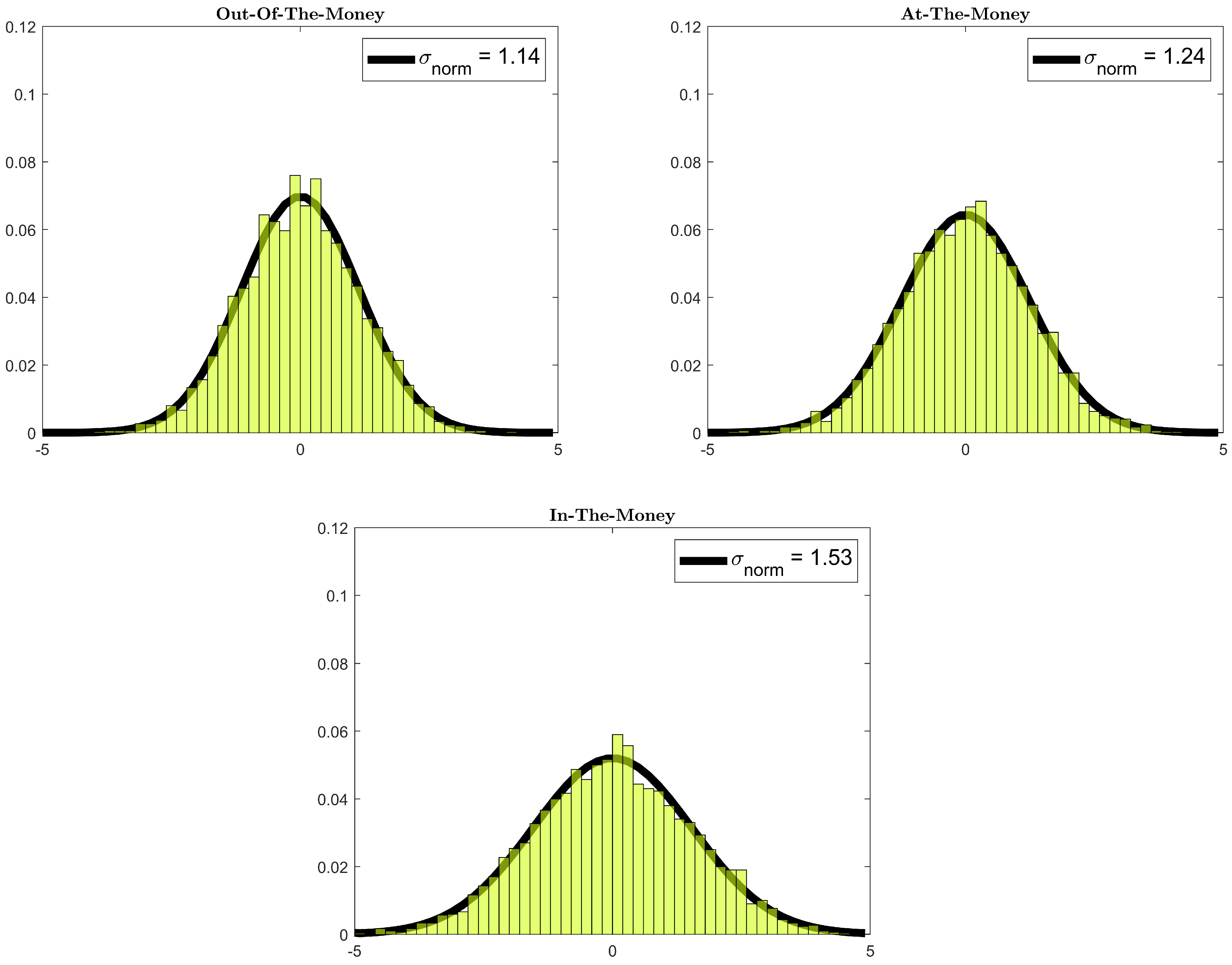
4.3. Calibration to SPX Options

In this section, we will calibrate the implied volatility under the rough Heston model computed through MLCV to the options of an index consisting of the top 500 companies in the U.S. market, which is the S&P 500 (SPX) option. The SPX options prices and stock are taken from the ending on 22 October 2021 with maturity dates ranging from $T=0.0992$ up to $T=0.4812$. The interest rate is assumed to be zero in the inversion of option price to implied volatility and computation of implied volatility through the rough Heston model. The main criterion of optimizing the parameters is the minimization of the root mean squared error between the bid-ask implied volatility. The calibrated parameters are as follows:

$$\begin{array}{cc}\hfill \alpha & =0.7600,\theta =0.0450,V_0=0.0095,\hfill \end{array}$$

(71)

$$\begin{array}{cc}\hfill \lambda & =2.0558,\nu =3.0480,\rho =-0.9507.\hfill \end{array}$$

(72)

Figure 5 shows the calibration of implied volatility under the rough Heston model to the SPX options against log-moneyness $log(K/S)$ (on the x-axis), using the MLCV Monte Carlo method. It shows that the calibrated implied volatility performs reasonably well for the different option maturities considered. It can be seen from Figure 5 that the implied volatility on $T=0.2579$ and $T=0.4812$ have some deviations at its end (in-the-money and out-of-the-money). One thing to take note of is that we have actually attempted to calibrate the rough Heston’s implied volatility, using MLCV up to maturity of $T=1.66$, but were unable to do so because of two main reasons: (1) with cost $C=1$ s, the implied volatility at larger maturity actually has large deviation, so the optimization algorithm simply would not work well with such a large deviation at each iteration; (2) there are six parameters to consider, and therefore, the optimization cost is extremely high. We are actually unsure whether the parameters in Equations (71) and (72) are even the global minimum of the optimization problem or not. We have tried three different optimization algorithms, including the gradient-based method (interior-point method), evolutionary algorithm (genetic algorithm), and pattern search algorithm. The gradient-based method obviously does not work well with stochastic problems, whereas the evolutionary algorithm simply requires extremely large computational cost to give a moderate optimal parameter. The parameters in Equations (71) and (72) are obtained through a pattern search algorithm with initial parameters given by the genetic algorithm.

5. Conclusions and Future Research

This paper mainly contributes to the Monte Carlo computation for option prices under the rough Heston model. In particular, we have proved finite bounds on t for the stochastic Volterra equation with a non-Lipschitz diffusion coefficient as well as the weak error and weak convergence of the discretization method. The proofs are located in the Appendix A and Appendix B. In addition, we have proposed a Control Variate estimator for variance reduction purpose and a mixed Monte Carlo method, which consists of the control variate method and multilevel method.

In Section 4, we conducted extensive numerical experiments that consider many scenarios, which we believe many readers or practitioners might find interesting. The most notable part is in Section 4.2, where all the computations and simulations are performed, using the cost-adjusted method rather than the number of simulations N. Time to time comparisons make it easier to identify which estimator is performing the best. In this case, the most favorable estimator goes to the proposed MLCV method. A substantial 17 times variance reduction can be achieved by using MLCV as compared to the BE. The numerical experiment for the discretization bias of the estimators was also conducted. The results show that there is little difference between $n=256$ and $n=1024$ in terms of discretization bias. A calibration of the SPX option was also performed on the MLCV Monte Carlo method at the end of Section 4. The overall performance of the calibration is overall satisfied, but there were some struggles in calibrating the optimal parameters.

We are aware that there was a recent study on an efficient simulation method of the stochastic Volterra equation [33] that used a hybrid exponential scheme. In particular, the author proved the convergence of the method with Lipschitz coefficient functions to the stochastic Volterra equation. The method can be potentially used to replace the discrete simulation of the stochastic Volterra equation for rough Heston volatility in practice once the convergence of the non-Lipschitz coefficient functions is proven. For future research, it would be interesting to see the hybrid exponential scheme [20,34] being used on a rough Heston model simulation and then consider the cost-adjusted performance of different estimators, including the proposed multilevel control variate estimator. In general, we also do hope to see improvements on the finite bound of $\mathbb{E}\left[\right|V_t-V_t^n{|}^p]$ or perhaps even strong convergence of the stochastic Volterra equation with a non-Lipschitz diffusion coefficient, i.e., ${lim}_{n\to \infty }\mathbb{E}\left[\right|V_t-V_t^n{|}^p]=0$. The main hurdle of proving the strong convergence in Lemma A1 is because we cannot use the Grönwall inequality to Equation (A37) the same way as we did to Equation (A49). Instead, we have to use Perov’s inequality to prove the convergence that is bounded on time t. In addition, Remark 2 indicates that the weak convergence rate of stochastic Volterra equation $|\mathbb{E}\left[V_t\right]-\mathbb{E}\left[V_t^n\right]|$ is of the order $O\left(n^{-H}\right)$, but in the study [35], the author proved that the discretization scheme of the Heston model (with $H=1/2$ in the stochastic Volterra process) under a certain hypothesis has a weak convergence rate of $O\left(n^{-1}\right)$. This indicates that the weak convergence rate of stochastic Volterra equation $|\mathbb{E}\left[V_t\right]-\mathbb{E}\left[V_t^n\right]|$ can potentially be improved to the order of $O\left(n^{-H-1/2}\right)$, which we leave for future work.

References

1. Gatheral, J.; Jaisson, T.; Rosenbaum, M. Volatility is rough. Quant. Financ. 2018, 18, 933–949. [Google Scholar] [CrossRef]
2. Comte, F.; Renault, E. Long memory in continuous-time stochastic volatility models. Math. Financ. 1998, 8, 291–323. [Google Scholar] [CrossRef]
3. Cheridito, P. Mixed fractional Brownian motion. Bernoulli 2001, 7, 913–934. [Google Scholar] [CrossRef]
4. Alòs, E.; León, J.A.; Vives, J. On the short-time behavior of the implied volatility for jump-diffusion models with stochastic volatility. Financ. Stoch. 2007, 11, 571–589. [Google Scholar] [CrossRef] [Green Version]
5. Fukasawa, M. Asymptotic analysis for stochastic volatility: Martingale expansion. Financ. Stoch. 2011, 15, 635–654. [Google Scholar] [CrossRef] [Green Version]
6. Bayer, C.; Friz, P.; Gatheral, J. Pricing under rough volatility. Quant. Financ. 2016, 16, 887–904. [Google Scholar] [CrossRef]
7. Bergomi, L. Smile Dynamics II. SSRN 2005. Available online: http://dx.doi.org/10.2139/ssrn.1493302 (accessed on 3 May 2021).
8. El Euch, O.; Fukasawa, M.; Rosenbaum, M. The microstructural foundations of leverage effect and rough volatility. Financ. Stoch. 2018, 22, 241–280. [Google Scholar] [CrossRef] [Green Version]
9. El Euch, O.; Rosenbaum, M. The characteristic function of rough Heston models. Math. Financ. 2019, 29, 3–38. [Google Scholar] [CrossRef] [Green Version]
10. El Euch, O.; Gatheral, J.; Radoicic, R.; Rosenbaum, M. The zumbach effect under rough heston. arXiv 2018, arXiv:1809.02098. Available online: https://arxiv.org/abs/1809.02098 (accessed on 2 April 2021). [CrossRef] [Green Version]
11. Gatheral, J.; Radoicic, R. Rational approximation of the rough Heston solution. Int. J. Theor. Appl. Financ. 2019, 22, 1950010. [Google Scholar] [CrossRef]
12. Jeng, S.W.; Kilicman, A. Approximation formula for option prices under rough heston model and short-time implied volatility behaviour. Symmetry 2020, 12, 1878. [Google Scholar] [CrossRef]
13. Jeng, S.W.; Kilicman, A. Fractional Riccati Equation and Its Applications to Rough Heston Model Using Numerical Methods. Symmetry 2020, 12, 959. [Google Scholar] [CrossRef]
14. Jeng, S.W.; Kilicman, A. Series Expansion and Fourth-Order Global Padé Approximation for a Rough Heston Solution. Mathematics 2020, 8, 1968. [Google Scholar] [CrossRef]
15. Abi Jaber, E. Lifting the Heston model. Quant. Financ. 2019, 19, 1995–2013. [Google Scholar] [CrossRef]
16. Giles, M.B. Multilevel monte carlo path simulation. Oper. Res. 2008, 56, 607–617. [Google Scholar] [CrossRef] [Green Version]
17. Giles, M.B. Multilevel monte carlo methods. Acta Numer. 2015, 24, 259. [Google Scholar] [CrossRef] [Green Version]
18. Glasserman, P. Monte Carlo Methods in Financial Engineering; Springer Science & Business Media: Berlin/Heidelberg, Germany, 2003; Volume 53. [Google Scholar]
19. Liu, G.; Zhao, Q.; Gu, G. A simple control variate method for options pricing with stochastic volatility models. Int. J. Appl. Math. 2015, 8, 1968. [Google Scholar]
20. McCrickerd, R.; Pakkanen, M.S. Turbocharging Monte Carlo pricing for the rough Bergomi model. Quant. Financ. 2018, 18, 1877–1886. [Google Scholar] [CrossRef] [Green Version]
21. Richard, A.; Tan, X.; Yang, F. Discrete-time simulation of stochastic volterra equations. arXiv 2020, arXiv:2004.00340. Available online: https://arxiv.org/abs/2004.00340 (accessed on 3 May 2021). [CrossRef]
22. El Euch, O.; Rosenbaum, M. Perfect hedging in rough Heston models. Ann. Appl. Probab. 2018, 28, 3813–3856. [Google Scholar] [CrossRef] [Green Version]
23. Forde, M.; Gerhold, S.; Smith, B. Small-time and large-time smile behaviour for the Rough Heston model. arXiv 2019, arXiv:1906.09034. Available online: https://arxiv.org/abs/1906.09034 (accessed on 25 April 2021).
24. Gatheral, J.; Keller-Ressel, M. Affine forward variance models. Financ. Stoch. 2018, 23, 501–533. [Google Scholar] [CrossRef] [Green Version]
25. Maruyama, G. Continuous markov processes and stochastic equations. Rend. Del Circ. Mat. Di Palermo 1955, 4, 48. [Google Scholar] [CrossRef]
26. Milstein, G. Approximate integration of stochastic differential equations. Theory Probab. Its Appl. 1975, 19, 557–562. [Google Scholar]
27. Richard, A.; Tan, X.; Yang, F. On the discrete-time simulation of the rough Heston model. arXiv 2021, arXiv:2107.07835. Available online: https://arxiv.org/abs/2107.07835 (accessed on 3 May 2021).
28. Milstein, G. A method of second-order accuracy integration of stochastic differential equations. Theory Probab. Its Appl. 1979, 23, 396–401. [Google Scholar] [CrossRef]
29. Talay, D. Efficient numerical schemes for the approximation of expectations of functionals of the solution of a sde, and applications. In Filtering and Control of Random Processes; Springer: Berlin/Heidelberg, Germany, 1984; pp. 294–313. [Google Scholar]
30. Shreve, S.E. Stochastic Calculus for Finance II: Continuous Time Models; Springer Science & Business Media: Berlin/Heidelberg, Germany, 2004; Volume 11. [Google Scholar]
31. Fairbanks, H.R.; Doostan, A.; Ketelsen, C.; Iaccarino, G. A low-rank control variate for multilevel Monte Carlo simulation of high-dimensional uncertain systems. J. Comput. Phys. 2017, 341, 121–139. [Google Scholar] [CrossRef] [Green Version]
32. Nobile, F.; Tesei, F. A Multi Level Monte Carlo method with control variate for elliptic PDEs with log-normal coefficients. Stoch. Partial Differ. Equ. Anal. Comput. 2015, 3, 398–444. [Google Scholar] [CrossRef]
33. Rømer, S.E. The Hybrid-Exponential Scheme for Stochastic Volterra Equations. SSRN 2020, ssrn.3706253. Available online: http://dx.doi.org/10.2139/ssrn.3706253 (accessed on 23 April 2021).
34. Bennedsen, M.; Lunde, A.; Pakkanen, M.S. Hybrid scheme for Brownian semistationary processes. Financ. Stoch. 2017, 21, 931–965. [Google Scholar] [CrossRef] [Green Version]
35. Alfonsi, A. On the discretization schemes for the CIR (and Bessel squared) processes. De Gruyter 2005, 355–384. [Google Scholar] [CrossRef]
36. Mitrinovic, D.S.; Pecaric, J.; Fink, A.M. Inequalities Involving Functions and Their Integrals and Derivatives; Springer Science & Business Media: Berlin/Heidelberg, Germany, 2012; Volume 53. [Google Scholar]
Figure 1. Implied volatility against log-strike log ( K / S ) plots on using α = { 0.6 , 0.8 } and ρ = { 0.6 , 0.2 } with different maturity time T.
Mathematics 09 02930 g001
Figure 2. Histograms and normal distribution fits of OTM, ATM and ITM ( k = log ( K / S ) = { 0.1053 , 0 , 0.0953 } ) implied volatility. The x-axis is 1000 ( σ i m p k σ ¯ i m p ) , whereas the y-axis is simply the probability that the implied volatility falls into the interval of the histogram. The σ n o r m is the standard deviation of the normal distribution fit.
Mathematics 09 02930 g002
Figure 3. Histograms and normal distribution fits of ATM implied volatility errors for base, control variate, multilevel and multilevel control variate estimator. The x-axis is transformed to 1000 ( σ i m p k σ ¯ i m p ) , whereas the y-axis is simply the probability that the implied volatility falls into the interval of the histogram. The σ n o r m is the standard deviation of the normal distribution fit.
Mathematics 09 02930 g003
Figure 4. Number of time steps or levels against the implied volatility plot to assess the discretization error.
Mathematics 09 02930 g004
Figure 5. Implied volatility surface of SPX options (22 October 2021) and its calibration. Red and blue solid lines are bid and ask implied volatilities respectively, whereas green-dashed line is implied volatility under the rough Heston model computed through the MLCV Monte Carlo method.
Mathematics 09 02930 g005