1. Preliminary Discussion
We are interested in the initial value problem (IVP) of the particular form:
where
and
. This equation is used to model a wide range of problems in science and engineering. We remark that
is absent from Equation (
1).
The Numerov method, which aids in advancing the numerical estimation of the solution from
to
, is one of the most well-known approaches for solving Equation (
1), is given by the formula:
with
and
. Remark also that
.
Hairer [
1], Chawla [
2] and Cash [
3] presented implicit Numerov-type techniques using off-step points for the first time around 40 years ago. The primary challenge at the time was dealing with the P-stability characteristic, which is important for addressing stiff oscillatory problems. Chawla [
4] presented the following modified Numerov scheme, which had the advantage of being evaluated explicitly:
with
h a steplength that remains constant through the integration of Equation (
1):
The vectors and are approximating and , respectively, while and are the function evaluations used by the method.
We utilize the known information at mesh according to
Since we have already computed in the previous step, we need only to evaluate and every step, and consequently, we spend only two stages per step.
Tsitouras then suggested a Runge–Kutta–Nyström (RKN)-style method [
5]. This technique significantly lowered the cost. As a result, just four steps are required to create a sixth-order method, whereas previous implementations required six function evaluations (see [
6]).
In the years that followed, our group delved thoroughly into the issue. Tsitouras developed eighth-order methods with nine steps per step in [
7]. Ninth-order methods were studied in [
8]. Simultaneously, a group of Spanish researchers published some highly interesting work on the same topic [
9,
10,
11].
In the present work, we intend to present a new method for addressing the problems with periodic solutions better. Traditionally, for achieving this, we try to fulfill various properties coming from a simple test equation. The main novelty here is that we will train the available free parameters in a wide set of relevant problems. For this training, we will use the differential evolution technique. It is believed that by using this methodology, we will conclude with a method better tuned for oscillatory problems.
2. Theory of Two-Step Hybrid Numerov-Type Methods
For numerically addressing Equation (
1), higher algebraic order methods are in great demand. We may express
t, which is the independent variable, as one of the components of
z. As a result, we concentrate without losing generality on the autonomous system
. Then, an
s-stages hybrid Numerov method may presented as [
7]:
with
the identity matrix,
the coefficient matrices of the method and
For the presentation of the coefficients, we make use of the Butcher tableau [
12,
13],
Method (
2) can be given using matrices [
8]. Since the function evaluations are computed sequentially, these methods are explicit. Thus,
D is strictly lower triangular matrix. When
, the associated matrices take the following form:
Since
is known from the previous step, four function evaluations are evaluated each step. For attaining sixth algebraic order, we must cancel the associated truncation error terms (see [
14]).
Seventeen parameters are shared by the scheme under examination. Namely, nine entries from the matrix
D (i.e.,
), five coefficients for vector
w and 3 coefficients for vector
a. However, in order to obtain 6th order, we must solve 23 condition equations (see Table 5 in [
14]).
The parameters are less than the equations. This is a usual problem while developing Runge–Kutta type methods. Using simplifying assumptions is a common way to get around this issue. We proceed setting,
Then we spend only the six parameters
,
,
and
to satisfy the above assumptions. Our profit is that all order conditions, including
and
, are discarded from the relevant list given in [
14]. As a result, only 9 order conditions remain to be satisfied by the remaining 11 coefficients.
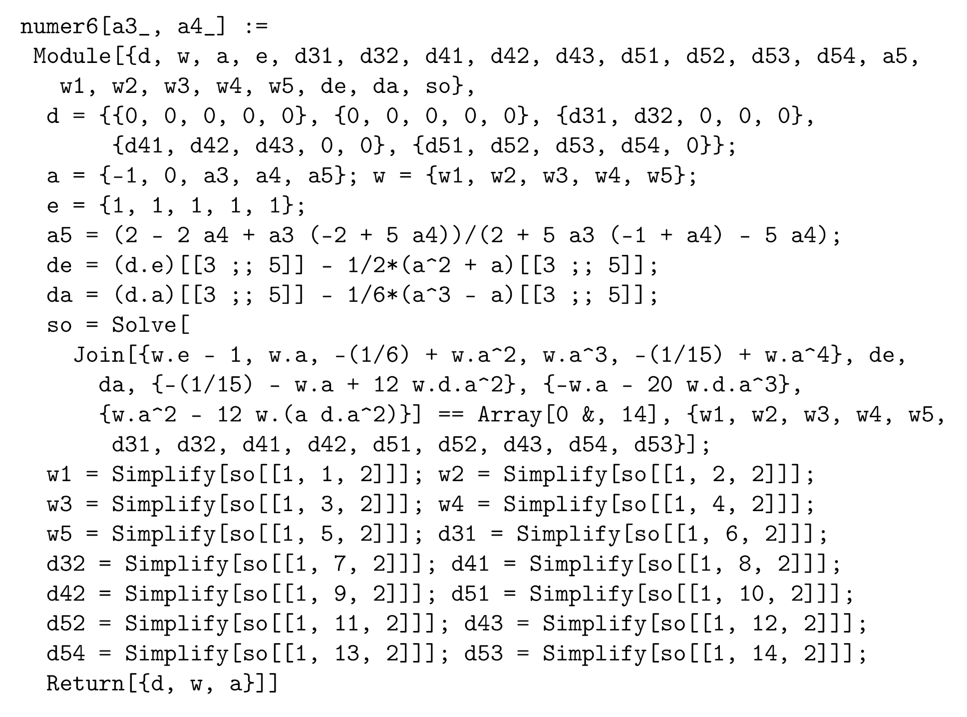
We select
and
as free parameters. The remainder of the coefficients are computed successively below through a Mathematica [
15] listing presented in
Figure 1.
For exhaustive information on the derivation of truncation error coefficients, see the review in [
14]. Through its link with the so-called T2 rooted trees, Coleman [
16] advocated using the B2 series representation of the local truncation error.
A first method from this family was given by Tsitouras [
5]. We may write in Mathematica the following lines and derive the method given in there.
In[1]:= numer6[1/2, -1/2] // AbsoluteTiming
Out[1]= {0.0141117, {
{{0, 0, 0, 0, 0},
{0, 0, 0, 0, 0},
{1/16, 5/16, 0, 0, 0},
{-(7/144), -(5/48), 1/36, 0, 0},
{-(2/9), 1/3, 2/9, 2/3, 0}},
{1/60, 13/30, 4/15, 4/15, 1/60},
{-1, 0, 1/2, -(1/2), 1}}}
Thus, we verify the efficiency of the algorithm since almost
seconds are enough for furnishing the coefficients in a Ryzen 9 3900X processor running at 3.79 GHz. Later, Franco [
9] chose
. These were all-purpose methods. In [
17], we proposed another approach for selecting
and
that concentrates on the method’s behavior in Keplerian type orbits. There we concluded that the choice
,
furnishes a method that best address the latter type of problems.
3. Performance of Methods in a Wide Set of Problems with Oscillating Solutions
From the above-mentioned family, we intend to develop a particular hybrid Numerov-type scheme. The resulting method has to perform best on problems with oscillating solutions. For this reason, we have chosen to test the following problems.
1–5.
The model problem
with the theoretical solution
. This problem was run for five different selections of
. Namely,
Thus, we obtain five problems 1–5.
6.
The inhomogeneous problem
with the theoretical solution
.
7. The Bessel equation
The wellknown Bessel equation
is verified by a theoretical solution of the form,
with
the zeroth-order Bessel function of the first kind. This equation in also integrated in the interval
.
8. The Duffing equation
Next, we choose the equation
with an approximate analytical solution given in [
14],
We again solved the above equation in the interval .
The three methods F6 [
9], M6 [
17] and T6 [
5] were run for the above problems and for different numbers for steps. The results in [
5,
9,
17] showed the superiority of the latter methods over the older schemes. The global errors over the whole mesh was recorded in
Table 1. Actually, we presented the errors in the form of the accurate digits observed. A final row with the mean value is also given in
Table 1.
In these 8 problems and for the 32 runs carried, it seems that T6 performed best. The question raised now is if we can do even better.
4. Phase-Lag and Amplification Errors
At first, we select a method of high phase-lag order. This means that we try to reduce the gap in the angle among the numerical and the theoretical solution in a free oscillator [
18]. The latter approach is well suited for use in problems with periodic solutions. Thus, after considering the test problem
and applying Method (
3), we verify as phase-lag the expression:
A sixth-order method shares sixth phase-lag order. Then after expanding with respect to
, we obtain
The equations for eighth and tenth phase-lag order are
and
respectively.
The only acceptable solution of
is
and
. However, we can not use such coefficients being so far away from the interval of interest
. Thus, we may draw back and accept only
by setting
We name this method PL8.
Another choice is the elimination of amplification errors. This is the distance from the orbit of the theoretical solution of a free oscillator. It is given as
Expanding with respect to
, we conclude to the exact form,
Unfortunately, we may not satisfy simultaneously and since we arrive at coefficients with indeterminate values. Thus, we may admit only by setting and . We name this method .
Another interesting property is P-stability [
2,
3]. Then, we have to satisfy
along with
Only implicit methods may address these two requirements simultaneously.
5. Training the Free Parameters in a Wide Set of Periodic Problems
Our current project’s initial concept is based on [
19]. After choosing the free parameters
, we obtain a method named NEW6 and form another column in
Table 1 for it. The average value
r obtained after the 32 runs may serve as a fitness measure and meant to be maximized. For the maximization process, we applied the differential evolution technique [
20].
DE is an iterative procedure, and in every iteration, named generation g, we work with a “population” of individuals , , with N the population size. An initial population , is randomly created in the first step of the method. We have also set the measure r as the fitness function, i.e., the average of accurate digits after the 32 runs mentioned above. The fitness function is then evaluated for each individual in the initial population. In each generation (iteration) g, a three-phases sequential scheme updates all of the individuals involved. These phases are Differentiation, Crossover and Selection.
We used MATLAB [
21] software DeMat [
22] for implementing the latter technique. Indeed, we manage to produce an improvement by choosing:
The coefficients of the new method in matrix forms are given below, which are suitable for double precision computations.
and
For this method, we obtained
, which is a very impressive result. Actually, we obtained many methods with
since there seems to exist a small area of pairs
, where
r attains high values. We also remark that for Selection (
4), the amplification is
and for phase lag
holds, i.e.,
, and no special property is satisfied.
We run the methods constructed for addressing periodic problems in the eight problems listed in
Section 3. We summarize the results in
Table 2. It is clear from this Table that NEW6 performs better than all methods referred until now. Namely, F6, M6, T6, PL8 and
.
Other authors have also tried recently to train coefficients of RK methods [
23]. However, in that later paper, only second- and third-order methods are considered [
24,
25] with constant step sizes and over single problems (e.g., Van der Pol). The learning algorithm given there remains to be tested on current and stiffer cases. Our proposal for differential evolution comes after several papers through the years [
19].
6. Numerical Results
Method NEW6 was produced to perform best on problems 1–8 listed in
Section 3. In the tests recorded in
Table 1 and
Table 2, it was meant to outperform other methods for the intervals and steps used there.
Thus, we intend to test NEW6 in a different set of problems, intervals and number of steps. In this direction, we run again problems 1–8 to the longer interval . We name these problems now . In addition, we included two nonlinear problems more.
9. Semi-Linear system.
The nonlinear problem proposed by Franco and Gomez [
26] follows:
with theoretical solution
10. Two coupled oscillators with different frequencies.
The problem is characterized by the equations [
27],
We also integrated this problem into
, but no analytical solution is available. For an estimation of the error in the grid points, we used a Runge–Kutta–Nyström method [
28] with very stringent tolerance.
11. Wave equation.
Finally, we consider the linearized wave equation, which is a rather large-scale problem [
14],
with the theoretical solution
We semi-discretisize
with fourth order symmetric differences at internal points and one sided differences of the same order at the boundaries (including the knowledge of
there) and conclude with the system:
By choosing , we arrive at a constant coefficients system with . The results for this problem were dominated by the semi-discretization errors.
We run these 11 problems for various numbers of steps and tabulated the results in
Table 3. There, we included results with other state-of-the-art methods considered in the area of sixth-order Numerov-type (i.e., including off step points) methods. It is obvious from there that NEW6 outperformed all other methods from the literature by a considerable distance.
7. Conclusions
The main points of our research was the following.
We considered a family of a sixth-order hybrid two-step scheme that shares the lowest number of stages, and the main novelty is suggesting a method for selecting proper free parameters.
The parameters of the new method were chosen after testing their performance in a large set of periodic problems.
The best choice was found using the differential evolution method. In a wide range of problems with oscillating solutions, the developed scheme significantly outperformed other methods from the same or other families.
The presented method is tuned for problems with periodic solutions, F especially when these problems share a large linear part.
Author Contributions
Conceptualization, V.N.K., T.E.S. and C.T.; Data curation, V.N.K., R.V.F., T.V.K. and T.E.S.; Formal analysis, V.N.K., R.V.F., T.V.K., T.E.S. and C.T.; Funding acquisition, T.E.S.; Investigation, V.N.K., R.V.F., T.V.K., T.E.S. and C.T.; Methodology, T.E.S. and C.T.; Project administration, T.E.S.; Resources, T.E.S. and C.T.; Software, R.V.F., T.V.K. and C.T.; Supervision, T.E.S.; Validation, V.N.K. and T.E.S.; Visualization, V.N.K., R.V.F. and T.E.S.; Writing—original draft, C.T.; Writing—review & editing, T.E.S. and C.T. All authors have contributed equally. All authors have read and agreed to the published version of the manuscript.
Funding
The research was supported by a Mega Grant from the Government of the Russian Federation within the framework of the federal project No. 075-15-2021-584.
Institutional Review Board Statement
Not applicable.
Informed Consent Statement
Not applicable.
Data Availability Statement
Not applicable.
Conflicts of Interest
The authors declare no conflict of interest.
References
- Hairer, E. Unconditionally stable methods for second order differential equations. Numer. Math. 1979, 32, 373–379. [Google Scholar] [CrossRef]
- Chawla, M.M. Two–step fourth order P–stable methods for second order differential equations. BIT 1981, 21, 190–193. [Google Scholar] [CrossRef]
- Cash, J.R. High order P–stable formulae for the numerical integration of periodic initial value problems. Numer. Math. 1981, 37, 355–370. [Google Scholar] [CrossRef]
- Chawla, M.M. Numerov Made Explicit has Better Stability. BIT 1984, 24, 117–118. [Google Scholar] [CrossRef]
- Tsitouras, C. Explicit Numerov type methods with reduced number of stages. Comput. Math. Appl. 2003, 45, 37–42. [Google Scholar] [CrossRef] [Green Version]
- Chawla, M.M.; Rao, P.S. An explicit sixth—Order method with phase—Lag of order eight for y′′=f(t,y). J. Comput. Appl. Math. 1987, 17, 365–368. [Google Scholar] [CrossRef] [Green Version]
- Tsitouras, C. Explicit eighth order two–step methods with nine stages for integrating oscillatory problems. Int. J. Modern Phys. C 2006, 17, 861–876. [Google Scholar] [CrossRef]
- Tsitouras, C.; Simos, T.E. On ninth order, explicit Numerov type methods with constant coefficients. Mediterr. J. Math. 2018, 15, 46. [Google Scholar] [CrossRef]
- Franco, J.M. A class of explicit two-step hybrid methods for second-order IVPs. J. Comput. Appl. Math. 2006, 187, 41–57. [Google Scholar] [CrossRef] [Green Version]
- Franco, J.M.; Randez, L. Explicit exponentially fitted two-step hybrid methods of high order for second-order oscillatory IVPs. Appl. Maths. Comput. 2016, 273, 493–505. [Google Scholar] [CrossRef]
- Franco, J.M.; Randez, L. Eighth-order explicit two-step hybrid methods with symmetric nodes and weights for solving orbital and oscillatory IVPs. Int. J. Modern. Phys. C 2018, 29, 1850002. [Google Scholar] [CrossRef]
- Butcher, J.C. Implicit Runge Kutta processes. Math. Comput. 1964, 18, 50–64. [Google Scholar]
- Butcher, J.C. On Runge–Kutta processes of high order. J. Austral. Math. Soc. 1994, 4, 179–194. [Google Scholar] [CrossRef] [Green Version]
- Simos, T.E.; Tsitouras, C.; Famelis, I.T. Explicit Numerov Type Methods with Constant Coefficients: A Review. Appl. Comput. Math. 2017, 16, 89–113. [Google Scholar]
- Wolfram Research Inc. Mathematica, Version 11.3; Wolfram Research Inc.: Champaign, IL, USA, 2018. [Google Scholar]
- Coleman, J.P. Order conditions for a class of two-step methods for y′′=f(x,y). IMA J. Numer. Anal. 2003, 23, 197–220. [Google Scholar] [CrossRef]
- Liu, C.; Hsw, C.W.; Tsitouras, C.; Simos, T.E. Hybrid Numerov-type methods with coefficients trained to perform better on classical orbits. B. Malays, Math. Sci. Soc. 2019, 42, 2119–2134. [Google Scholar] [CrossRef]
- Chawla, M.M.; Rao, P.S. Numerov-type method with minimal phase-lag for the integration of second order periodic initial value problems. J. Comput. Appl. Math. 1984, 11, 277–281. [Google Scholar] [CrossRef] [Green Version]
- Tsitouras, C. Neural Networks With Multidimensional Transfer Functions. IEEE T. Neural Nets 2002, 13, 222–228. [Google Scholar] [CrossRef]
- Storn, R.; Price, K. Differential evolution—A simple and efficient heuristic for global optimization over continuous spaces. J. Glob. Optim. 1997, 11, 341–359. [Google Scholar] [CrossRef]
- MATLAB Version R2019b. Available online: https://www.mathworks.com/products/new_products/release2019b.html (accessed on 23 August 2021).
- DeMat. Available online: https://www.swmath.org/software/24853 (accessed on 23 August 2021).
- Guo, Y.; Dietrich, F.; Bertalan, T.; Doncevic, D.T.; Dahmen, M.; Kevrekidis, I.G. Personalized Algorithm Generation: A Case Study in Meta-Learning ODE Integrators. arXiv 2021, arXiv:2105.01303v1. [Google Scholar]
- Runge, C. Ueber die numerische Auflöung von Differentialgleichungen. Math. Ann. 1895, 46, 167–178. [Google Scholar] [CrossRef] [Green Version]
- Kutta, W. Beitrag zur naherungsweisen Integration von Differentialgleichungen. Z. Math. Phys. 1901, 46, 435–453. [Google Scholar]
- Franco, J.M.; Gomez, I. Trigonometrically fitted nonlinear two-step methods for solving second order oscillatory IVPs. Appl. Math. Comput. 2014, 232, 643–657. [Google Scholar] [CrossRef]
- Vigo-Aguiar, J.; Simos, T.E.; Ferrndiz, J.M. Controlling the error growth in long-term numerical integration of perturbed oscillations in one or several frequencies. Proc. R. Soc. Lond. A 2004, 460, 561–567. [Google Scholar] [CrossRef]
- Dormand, J.R.; El-Mikkawy, M.E.A.; Prince, P.J.C. High-Order Embedded Runge-Kutta and Nyström pairs. IMA J. Numer. Anal. 1987, 7, 423–430. [Google Scholar] [CrossRef]
| Publisher’s Note: MDPI stays neutral with regard to jurisdictional claims in published maps and institutional affiliations. |
© 2021 by the authors. Licensee MDPI, Basel, Switzerland. This article is an open access article distributed under the terms and conditions of the Creative Commons Attribution (CC BY) license (https://creativecommons.org/licenses/by/4.0/).


 ,
, 
