Adjustment of Force–Gradient Operator in Symplectic Methods

Abstract

Many force–gradient explicit symplectic integration algorithms have been designed for the Hamiltonian $H=T\left(\mathbf{p}\right)+V\left(\mathbf{q}\right)$ with kinetic energy $T\left(\mathbf{p}\right)={\mathbf{p}}^2/2$ in the existing references. When a force–gradient operator is appropriately adjusted as a new operator, it is still suitable for a class of Hamiltonian problems $H=K(\mathbf{p},\mathbf{q})+V\left(\mathbf{q}\right)$ with integrable part $K(\mathbf{p},\mathbf{q})={\sum }_{i=1}^n{\sum }_{j=1}^n{a}_{ij}{p}_i{p}_j+{\sum }_{i=1}^n{b}_i{p}_i$, where $a_{ij}=a_{ij}\left(\mathbf{q}\right)$ and $b_i=b_i\left(\mathbf{q}\right)$ are functions of coordinates $\mathbf{q}$. The newly adjusted operator is not a force–gradient operator but is similar to the momentum-version operator associated to the potential V. The newly extended (or adjusted) algorithms are no longer solvers of the original Hamiltonian, but are solvers of slightly modified Hamiltonians. They are explicit symplectic integrators with symmetry or time reversibility. Numerical tests show that the standard symplectic integrators without the new operator are generally poorer than the corresponding extended methods with the new operator in computational accuracies and efficiencies. The optimized methods have better accuracies than the corresponding non-optimized counterparts. Among the tested symplectic methods, the two extended optimized seven-stage fourth-order methods of Omelyan, Mryglod and Folk exhibit the best numerical performance. As a result, one of the two optimized algorithms is used to study the orbital dynamical features of a modified Hénon–Heiles system and a spring pendulum. These extended integrators allow for integrations in Hamiltonian problems, such as the spiral structure in self-consistent models of rotating galaxies and the spiral arms in galaxies.

1. Introduction

In some cases, many trajectories of nonlinear ordinary differential dynamical systems exhibit chaotic behavior; namely, the separations between the trajectories and their nearby trajectories display exponentially sensitive dependence on initial conditions. The trajectories are not analytically integrable, and therefore their studies mainly rely on numerical integration schemes. In general, detecting the chaotic behavior needs long enough numerical integrations with reliable results. Thus, the adopted computational schemes must perform with good stability and high precision. An eighth- and ninth-order Runge–Kutta–Fehlberg integrator [RKF8(9)] with adaptive step sizes significantly improves the accuracies of the integrals of motion and the trajectories. However, the higher-precision solutions come at the expense of computational time. Furthermore, lower-order numerical methods that preserve geometric properties of the flow of differential equations, i.e., geometric numerical integration schemes [1], are often employed to achieve very accurate long-time determination of the trajectories. The geometric integrators include symplectic integrators for Hamiltonian systems [2,3,4], symmetric integrators for reversible systems, manifold correction schemes for the consistency of integrals (or quasi integrals) of motion [5,6], energy-preserving methods [7], etc.

When dealing with Hamiltonian systems, symplectic integrators are the most appropriate geometric solvers, which own the symplectic nature of Hamiltonian dynamics. The errors in the integrals of motion involving energy integral have no secular growth and tend to zero for infinitesimal time steps. In this sense, symplectic methods approximately conserve the integrals of motion. There are implicit symplectic schemes for inseparable Hamiltonian systems, and explicit symplectic schemes for integrable separable Hamiltonian systems. The implicit schemes were developed by Feng and Qin [8] using generating functions. Implicit symplectic Runge–Kutta methods including the second-order implicit midpoint rule were presented by Sanz-Serna [9]. The family of Gauss–Legndre Runge–Kutta methods [10] are also symplectic. These implicit methods are applied to full Hamiltonian systems. If a part of the Hamiltonian systems is explicitly solved and another part of the Hamiltonian systems is implicitly solved, then explicit and implicit combined symplectic methods [11,12,13] are obtained and can reduce the expense of computational time, compared with the implicit symplectic methods for the full Hamiltonian systems.

Are symplectic integrations always implicit for nonseparable Hamiltonians? No, they are not. In fact, explicit symplectic integrations have been possibly available for some nonseparable Hamiltonians [14]. Relatively recently, explicit symplectic integrators were designed for the Hamiltonian of Schwarzschild spacetime split into four integrable parts [15]. There are a class of explicit extended phase-space symplectic or symplectic-like integrations [16] for an arbitrary separable or inseparable Hamiltonian system. Of course, explicit symplectic integrations are less computationally expensive in general than same order implicit symplectic integrations.

Naturally, explicit symplectic integrations are extensively applied to separable Hamiltonians. Ruth [3] proposed second- and third-order explicit symplectic methods for Hamiltonian systems of the form $H=T\left(\mathbf{p}\right)+V\left(\mathbf{q}\right)$. Along this direction, higher order standard explicit symplectic schemes were developed by many authors [17,18,19,20]. It is worth emphasizing that Ruth [3] also gave another third-order symplectic algorithm in which the computation of force gradient is included. Such construction is the force–gradient symplectic integrator. Based on this idea, a series of higher order explicit force–gradient symplectic integration algorithms were established and applied by several authors [21,22,23]. Positive time coefficients can be admissible in many of the algorithmic constructions. In view of this, the force–gradient algorithms with positive intermediate time-steps are suitable for solving time-irreversible problems, such as imaginary time Schrödinger equations. A force–gradient explicit symplectic integration needs less exponential functions of Lie operators than a same order standard explicit symplectic integration. The former algorithm is generally superior to the latter one at same order in accuracy.

When dealing with Hamiltonian systems with the integrable perturbation decomposition form $H=H_0(\mathbf{p},\mathbf{q})+ϵH_1\left(\mathbf{q}\right)$, the Wisdom-Holman symplectic map of second order [24] drastically improves the numerical accuracy, compared with the standard explicit symplectic method of second order for the Hamiltonian splitting form $H=T\left(\mathbf{p}\right)+V\left(\mathbf{q}\right)$. According to the perturbation decomposition of Hamiltonian systems, a number of higher order explicit symplectic integrations were developed and generalized in some references [25,26].

It can be seen from the above presentations that the construction of symplectic integrators is closely related to Hamiltonian systems or their splitting forms. In this contribution, we plan to develop explicit force–gradient symplectic integration algorithms for Hamiltonian systems of the form $H=K(\mathbf{p},\mathbf{q})+V\left(\mathbf{q}\right)$ with integrable kinetic energy $K(\mathbf{p},\mathbf{q})={\sum }_{i=1}^n{\sum }_{j=1}^n{a}_{ij}{p}_i{p}_j+{\sum }_{i=1}^n{b}_i{p}_i$, where $a_{ij}=a_{ij}\left(\mathbf{q}\right)$ and $b_i=b_i\left(\mathbf{q}\right)$. Because this Hamiltonian is different from the Hamiltonian $H=T\left(\mathbf{p}\right)+V\left(\mathbf{q}\right)$, the force–gradient operator for the latter Hamiltonian should be modified appropriately in the former Hamiltonian.

The remainder of the present paper is organized as follows. The force–gradient operator is extended or adjusted in Section 2. Taking two models, we estimate the numerical performance of some extended version fourth-order force–gradient symplectic integrators in Section 3. For comparison, the standard fourth-order symplectic method of Forest & Ruth [17] and its optimized methods [20] are employed. Possible differences in the dynamics of order and chaos among the tested symplectic integrators are compared, and the dynamics of the two systems is truly described. Finally, the main results are concluded in Section 4.

2. Extension of Force–Gradient Operator

In this Section, some known force–gradient symplectic integrators are introduced. Then, their applications are extended. In what follows, the symplecticity of the extended algorithms is clearly shown.

2.1. Existing Force–Gradient Symplectic Integrators

A kinetic energy $T\left(\mathbf{p}\right)$ is a quadratic function of n-dimensional momentum vector $\mathbf{p}=(p_1,\cdots ,p_n)$

$$T\left(\mathbf{p}\right)=\frac{1}{2}{\mathbf{p}}^2,$$

(1)

and a potential energy $V\left(\mathbf{q}\right)$ depends on coordinate $\mathbf{q}=(q_1,\cdots ,q_n)$ only. T and V determine a Hamiltonian

$$H(\mathbf{p},\mathbf{q})=T\left(\mathbf{p}\right)+V\left(\mathbf{q}\right).$$

(2)

Lie derivative operators of T and V are defined as

$$\begin{array}{ccc}\hfill A& =& \{,T\}=\sum _{i=1}^n{T}_{p_i}\frac{\partial }{\partial q_i},\hfill \end{array}$$

(3)

$$\begin{array}{ccc}\hfill B& =& \{,V\}=-\sum _{i=1}^n{V}_{q_i}\frac{\partial }{\partial p_i},\hfill \end{array}$$

(4)

where $T_{p_i}=\partial T/\partial p_i=p_i$, $V_{q_i}=\partial V/\partial q_i$, and symbols $\{,\}$ denote Poisson brackets. Applying Lie derivative A to act on coordinates $q_i$ and momenta $p_i$, we obtain ${\dot{q}}_i=A{q}_i=T_{p_i}=p_i$ and ${\dot{p}}_i=A{p}_i=0$. Clearly, A is a position-version operator. In other words, T has an analytical solution as an explicit function of time. Because $B{p}_i=-V_{q_i}$ and $B{q}_i=0$, B is a momentum-version operator and is easily analytically solved.

The two operators A and B can symmetrically compose a second-order Verlet symplectic integrator [27]

$$\begin{array}{c}\hfill \mathrm{M}2=e^W=e^{\frac{\tau }{2}B}{e}^{\tau A}{e}^{\frac{\tau }{2}B},\end{array}$$

(5)

where $\tau$ is a step size, and W is written in terms of Baker-Campbell-Hausdroff (BCH) formula as

$$\begin{array}{ccc}\hfill W& =& \tau (A+B)+{\tau }^3(-\frac{1}{12}[A,[B,A]]\hfill \\ & & +\frac{1}{24}[B,[A,B]])+\mathcal{O}\left({\tau }^5\right).\hfill \end{array}$$

(6)

The two operators can also symmetrically compose fourth-order explicit symplectic algorithms, such as the Forest-Ruth method [17]

$$\begin{array}{ccc}\hfill \mathrm{M}4& =& e^{\alpha \tau A}{e}^{\beta \tau B}{e}^{(\frac{1}{2}-\alpha )\tau A}{e}^{(1-2\beta )\tau B}\hfill \\ & & \times e^{(\frac{1}{2}-\alpha )\tau A}{e}^{\beta \tau B}{e}^{\alpha \tau A},\hfill \end{array}$$

(7)

where $\beta =1/(2-\sqrt[3]{2})$ and $\alpha =\beta /2$. An optimized Forest-Ruth-like explicit symplectic algorithm of order 4 in [20] is

$$\begin{array}{ccc}\hfill \mathrm{M}4\mathrm{V}& =& e^{\xi \tau B}{e}^{(1-2\lambda )\frac{\tau }{2}A}{e}^{\chi \tau B}{e}^{\lambda \tau A}{e}^{(1-2(\chi +\xi \left)\right)\tau B}\hfill \\ & & \times e^{\lambda \tau A}{e}^{\chi \tau B}{e}^{(1-2\lambda )\frac{\tau }{2}A}{e}^{\xi \tau B},\hfill \end{array}$$

(8)

where time coefficients are

$$\begin{array}{ccc}\hfill \xi & =& 0.1644986515575760E+00,\hfill \\ \hfill \lambda & =& -0.2094333910398989E-01,\hfill \\ \hfill \chi & =& +0.1235692651138917E+01.\hfill \end{array}$$

In fact, only two of the three coefficients sufficiently satisfy the conditions for order 4. In this case, one of the three coefficients has a free choice. However, the free coefficient such as $\xi$ can be determined when the norm of the leading term of fifth-order truncation errors is minimized. This is the so-called optimized method. Another optimized algorithm of order 4 is

$$\begin{array}{ccc}\hfill \mathrm{M}4\mathrm{P}& =& e^{\xi \tau A}{e}^{(1-2\lambda )\frac{\tau }{2}B}{e}^{\chi \tau A}{e}^{\lambda \tau B}{e}^{(1-2(\chi +\xi \left)\right)\tau A}\hfill \\ & & \times e^{\lambda \tau B}{e}^{\chi \tau A}{e}^{(1-2\lambda )\frac{\tau }{2}B}{e}^{\xi \tau A},\hfill \end{array}$$

(9)

where time coefficients are

$$\begin{array}{ccc}\hfill \xi & =& 0.1786178958448091\times {10}^0,\hfill \\ \hfill \lambda & =& -0.2123418310626054\times {10}^0,\hfill \\ \hfill \chi & =& -0.6626458266981849\times {10}^{-1}.\hfill \end{array}$$

Explicit symplectic algorithms to arbitrary even orders were given in [18,19].

Let us consider one of the truncation error terms about ${\tau }^3$ in Equation (6). In terms of commutator $[A,B]=AB-BA$, we have a commutator $C=[B,[A,B\left]\right]=[B,AB-BA]=2BAB-BBA-ABB$. It is easy to derive the following results: $ABB{q}_i=ABB{p}_i\equiv 0$, $BAB{q}_i\equiv 0$, $BBA{q}_i=BBA{p}_i\equiv 0$, and

$$\begin{array}{c}\hfill BAB{p}_i=\sum _{j=1}^n{V}_{q_i{q}_j}{V}_{q_j}.\end{array}$$

(10)

Thus, C is still a momentum-version operator

$$\begin{array}{ccc}\hfill C& =& 2BAB\hfill \\ \hfill & =& \sum _{i=1}^n\sum _{j=1}^{n}2V_{q_i{q}_j}{V}_{q_j}\frac{\partial }{\partial p_i}\hfill \\ & =& \sum _{i=1}^n{\nabla }_i{\mathbf{f}}^2\frac{\partial }{\partial p_i},\hfill \end{array}$$

(11)

where $V_{q_i{q}_j}={\partial }^{2}V/\partial q_i\partial q_j$, and $\mathbf{f}=(f_1,\cdots ,f_n)$ with ${\mathbf{f}}_j=-V_{q_j}$ is a component of the force governed by potential V. That is to say, C is a momentum-version operator with respect to the gradient of the square of force. In this sense, C is called as a force–gradient operator in [21,22,23].

The above demonstrations show that the third-order truncation error term C in the second-order method M2 and B belong to momentum-version operators. This means that a combination of B and C can yield higher-order algorithms. For example,

$$\begin{array}{c}\hfill \mathrm{F}2=e^{\frac{\tau }{2}(B+\frac{{\tau }^2}{24}C)}{e}^{\tau A}{e}^{\frac{\tau }{2}(B+\frac{{\tau }^2}{24}C)}\end{array}$$

(12)

is a second-order algorithm which eliminates the error term $[B,[A,B\left]\right]$ in Equation (6). If the error term $[A,[B,A\left]\right]$ in Equation (6) is also eliminated, a five-stage fourth-order method is Chin’s construction [21]

$$\begin{array}{c}\hfill \mathrm{F}4=e^{\frac{\tau }{2}\left(1-\frac{1}{\sqrt{3}}\right)A}{e}^{\frac{\tau }{2}(B+\frac{{\tau }^2}{24}(2-\sqrt{3})C)}\\ \hfill \times e^{\frac{\tau }{\sqrt{3}}A}{e}^{\frac{\tau }{2}(B+\frac{{\tau }^2}{24}(2-\sqrt{3})C)}{e}^{\frac{\tau }{2}\left(1-\frac{1}{\sqrt{3}}\right)A}.\end{array}$$

(13)

When $A\leftrightarrow B$ in Equation (13), there is another five-stage fourth-order scheme

$$\begin{array}{c}\hfill {\mathrm{F}4}^{*}=e^{\frac{\tau }{6}(B+\frac{{\tau }^2}{72}C)}{e}^{\frac{\tau }{2}A}{e}^{\frac{2\tau }{3}[B+\frac{{\tau }^2}{72}C]}{e}^{\frac{\tau }{2}A}{e}^{\frac{\tau }{6}[B+\frac{{\tau }^2}{72}C]}.\end{array}$$

(14)

An optimized five-stage fourth-order method with the operator C [23] is

$$\begin{array}{ccc}\hfill \mathrm{F}4\mathrm{O}& =& e^{\lambda \tau [B+(6\xi +k){\tau }^{2}C]}{e}^{\frac{\tau }{2}A}{e}^{(1-2\lambda )\tau [B+(6\xi +k){\tau }^{2}C]}\hfill \\ & & \times e^{\frac{\tau }{2}A}{e}^{\lambda \tau [B+(6\xi +k){\tau }^{2}C]},\hfill \end{array}$$

(15)

where $\lambda =1/6$, $\xi =-$17/18,000, $\chi =71/4500$, and $k=-4\xi -\frac{1}{2}+\frac{3\chi }{2}$. The choice of $\xi$ minimizes the norm of the leading term of fifth-order truncation errors. Two optimized seven-stage fourth-order methods with the operator C in [23] are

$$\begin{array}{ccc}\hfill \mathrm{F}4\mathrm{V}& =& e^{\lambda \tau [B+2(\xi +\chi ){\tau }^{2}C]}{e}^{\theta \tau A}{e}^{(1-2\lambda )\frac{\tau }{2}[B+2(\xi +\chi ){\tau }^{2}C]}\hfill \\ & & \times e^{(1-2\theta )\tau A}{e}^{(1-2\lambda )\frac{\tau }{2}[B+2(\xi +\chi ){\tau }^{2}C]}{e}^{\theta \tau A}\hfill \\ & & \times e^{\lambda \tau [B+2(\xi +\chi ){\tau }^{2}C]},\hfill \end{array}$$

(16)

where

$$\begin{array}{ccc}\hfill \theta & =& 0.2728983001988755\times {10}^0,\hfill \\ \hfill \lambda & =& 0.8002565306418866\times {10}^{-1},\hfill \\ \hfill \chi & =& 0.2960781208329478\times {10}^{-2},\hfill \\ \hfill \xi & =& 0.2725753410753895\times {10}^{-3},\hfill \end{array}$$

and

$$\begin{array}{ccc}\hfill \mathrm{F}4\mathrm{P}& =& e^{\theta \tau A}{e}^{\lambda \tau [B+(2\xi +\chi ){\tau }^{2}C]}{e}^{(1-2\theta )\frac{\tau }{2}A}\hfill \\ & & \times e^{(1-2\lambda )\tau [B+(2\xi +\chi ){\tau }^{2}C]}{e}^{(1-2\theta )\frac{\tau }{2}A}\hfill \\ & & \times e^{\lambda \tau [B+(2\xi +\chi ){\tau }^{2}C]}{e}^{\theta \tau A},\hfill \end{array}$$

(17)

where

$$\begin{array}{ccc}\hfill \theta & =& 0.1159953608486416\times {10}^0,\hfill \\ \hfill \lambda & =& 0.2825633404177051\times {10}^0,\hfill \\ \hfill \chi & =& 0.3035236056708454\times {10}^{-2},\hfill \\ \hfill \xi & =& 0.1226088989536361\times {10}^{-2}.\hfill \end{array}$$

Note that the combinations of B and C in Equations (15)–(17) are slightly unlike those in [23], but the time coefficients are the same as those in [23]. While the three methods F4O, F4V and F4P are optimized algorithms, their differences are that a free coefficient for F4O minimizes the norm of the leading term of fifth-order truncation errors, but two free coefficients such as $\xi$ and $\chi$ for F4V and F4P do.

Algorithms (12)–(17) with the force–gradient operator C are the so-called force–gradient explicit symplectic methods in the known publications (e.g., [21,22,23]). Their constructions are based on one of the third-order truncation error terms in the second-order method M2 included in the potential energy. Only the time coefficient $\lambda (6\xi +k)$ with respect to the operator C in Equation (15) is negative, but the time coefficients with respect to the operators A and B in Equations (12)–(17) and the time coefficients with respect to the operator C in Equations (12)–(14), (16) and (17) are positive. Thus, no F4O but F2, F4, F4${}^{*}$, F4V and F4P can have positive intermediate time-steps.

2.2. Adjustment of the Force–Gradient Operator

Now, let us suppose a Hamiltonian

$$\begin{array}{ccc}\hfill J(\mathbf{p},\mathbf{q})& =& K(\mathbf{p},\mathbf{q})+V\left(\mathbf{q}\right),\hfill \end{array}$$

(18)

$$\begin{array}{ccc}\hfill K(\mathbf{p},\mathbf{q})& =& \sum _{i=1}^n\sum _{j=1}^n{a}_{ij}{p}_i{p}_j+\sum _{i=1}^n{b}_i{p}_i,\hfill \end{array}$$

(19)

where $a_{ij}=a_{ij}\left(\mathbf{q}\right)$ and $b_i=b_i\left(\mathbf{q}\right)$. $K(\mathbf{p},\mathbf{q})$ is a formal kinetic energy unlike the kinetic energy in Equation (1). It is a quadratic function of the momentum vector $\mathbf{p}$, and also depends on the coordinate vector $\mathbf{q}$.

Lie derivative operator of K is expressed as

$$\begin{array}{ccc}\hfill A& =& \{,K\}=\sum _{i=1}^n\left(K_{p_i}\frac{\partial }{\partial q_i}-K_{q_i}\frac{\partial }{\partial p_i}\right),\hfill \end{array}$$

(20)

where $K_{p_i}=\partial K/\partial p_i$ and $K_{q_i}=\partial K/\partial q_i$. We have ${\dot{q}}_i=A{q}_i=K_{p_i}$ and ${\dot{p}}_i=A{p}_i=-K_{q_i}$. In this sense, A is a momentum- and position-version mixed operator. If K is nonlinear, it is not necessarily analytically solved. Here, K is assumed to have an analytical solution as an explicit function of time, i.e., operator A is analytically solvable. Taking $D=[B,[A,B\left]\right]=[B,AB-BA]=2BAB-BBA-ABB$, we obtain the results as follows: $ABB{q}_i=ABB{p}_i\equiv 0$, $BAB{q}_i\equiv 0$, $BBA{q}_i\equiv 0$, and

$$\begin{array}{ccc}\hfill BAB{p}_i& =& \sum _{j=1}^n\sum _{k=1}^n{V}_{q_i{q}_j}{V}_{q_k}{K}_{p_j{p}_k},\hfill \end{array}$$

(21)

$$\begin{array}{ccc}\hfill BBA{p}_i& =& -\sum _{j=1}^n\sum _{k=1}^n{V}_{q_j}{V}_{q_k}{K}_{q_i{p}_j{p}_k},\hfill \end{array}$$

(22)

where $K_{p_j{p}_k}=\frac{{\partial }^{2}K}{\partial p_j\partial p_k}$ and $K_{q_i{p}_j{p}_k}=\frac{{\partial }^{3}K}{\partial q_i\partial p_j\partial p_k}$. Thus, D is still a momentum-version operator

$$\begin{array}{ccc}\hfill D& =& 2BAB-BBA\hfill \\ \hfill & =& \sum _{i=1}^n\sum _{j=1}^n\sum _{k=1}^n(2V_{q_i{q}_j}{V}_{q_k}{K}_{p_j{p}_k}\hfill \\ & & +V_{q_j}{V}_{q_k}{K}_{q_i{p}_j{p}_k})\frac{\partial }{\partial p_i}.\hfill \end{array}$$

(23)

Obviously, D is different from the force–gradient operator C. It is an extended or adjusted operator of the force–gradient operator C.

Algorithms (12)–(17) with the force–gradient operator C become useless for the Hamiltonian J without doubt. However, when the force–gradient operator C is replaced with the extended operator D, these integrators are still available for the Hamiltonian J. That is, they correspond in sequence to the following forms

$$\begin{array}{c}\hfill \mathrm{N}2=e^{\frac{\tau }{2}(B+\frac{{\tau }^2}{24}D)}{e}^{\tau A}{e}^{\frac{\tau }{2}(B+\frac{{\tau }^2}{24}D)},\end{array}$$

(24)

$$\begin{array}{c}\hfill \mathrm{N}4=e^{\frac{\tau }{2}\left(1-\frac{1}{\sqrt{3}}\right)A}{e}^{\frac{\tau }{2}(B+\frac{{\tau }^2}{24}(2-\sqrt{3})D)}\\ \hfill \times e^{\frac{\tau }{\sqrt{3}}A}{e}^{\frac{\tau }{2}(B+\frac{{\tau }^2}{24}(2-\sqrt{3})D)}{e}^{\frac{\tau }{2}\left(1-\frac{1}{\sqrt{3}}\right)A},\end{array}$$

(25)

$$\begin{array}{c}\hfill {\mathrm{N}4}^{*}=e^{\frac{\tau }{6}(B+\frac{{\tau }^2}{72}D)}{e}^{\frac{\tau }{2}A}{e}^{\frac{2\tau }{3}[B+\frac{{\tau }^2}{72}D]}{e}^{\frac{\tau }{2}A}{e}^{\frac{\tau }{6}[B+\frac{{\tau }^2}{72}D]},\end{array}$$

(26)

$$\begin{array}{ccc}\hfill \mathrm{N}4\mathrm{O}& =& e^{\lambda \tau [B+(6\xi +k){\tau }^{2}D]}{e}^{\frac{\tau }{2}A}{e}^{(1-2\lambda )\tau [B+(6\xi +k){\tau }^{2}D]}\hfill \\ & & \times e^{\frac{\tau }{2}A}{e}^{\lambda \tau [B+(6\xi +k){\tau }^{2}D]},\hfill \end{array}$$

(27)

$$\begin{array}{ccc}\hfill \mathrm{N}4\mathrm{V}& =& e^{\lambda \tau [B+2(\xi +\chi ){\tau }^{2}D]}{e}^{\theta \tau A}{e}^{(1-2\lambda )\frac{\tau }{2}[B+2(\xi +\chi ){\tau }^{2}D]}\hfill \\ & & \times e^{(1-2\theta )\tau A}{e}^{(1-2\lambda )\frac{\tau }{2}[B+2(\xi +\chi ){\tau }^{2}D]}{e}^{\theta \tau A}\hfill \\ & & \times e^{\lambda \tau [B+2(\xi +\chi ){\tau }^{2}D]},\hfill \end{array}$$

(28)

$$\begin{array}{ccc}\hfill \mathrm{N}4\mathrm{P}& =& e^{\theta \tau A}{e}^{\lambda \tau [B+(2\xi +\chi ){\tau }^{2}D]}{e}^{(1-2\theta )\frac{\tau }{2}A}\hfill \\ & & \times e^{(1-2\lambda )\tau [B+(2\xi +\chi ){\tau }^{2}D]}{e}^{(1-2\theta )\frac{\tau }{2}A}\hfill \\ & & \times e^{\lambda \tau [B+(2\xi +\chi ){\tau }^{2}D]}{e}^{\theta \tau A}.\hfill \end{array}$$

(29)

Higher-order force–gradient algorithms in [22,23] can become the extended methods similar to the constructions (25)–(29).

The time coefficients of the composite operators A, B and D in each of the newly extended methods (24)–(29) correspond to those in the existing force–gradient algorithms (12)–(17). No N4O but N2, N4, N4${}^{*}$, N4V and N4P can have positive intermediate time-steps. These extended methods are symmetric or time-reversible. The condition for symmetry or time-reversibility is, e.g., $\mathrm{N}4\mathrm{O}\left(\tau \right)\times \mathrm{N}4\mathrm{O}(-\tau )=id$ for the method N4O [1], where id denotes an identical map. The condition is easily checked from a theoretical point of view because the exponents of these operators are linear combinations of $\tau$ and ${\tau }^3$ terms. If the exponents include even power terms of $\tau$ such as ${\tau }^2$ and ${\tau }^4$ terms, then the condition for symmetry or time-reversibility is not satisfied.

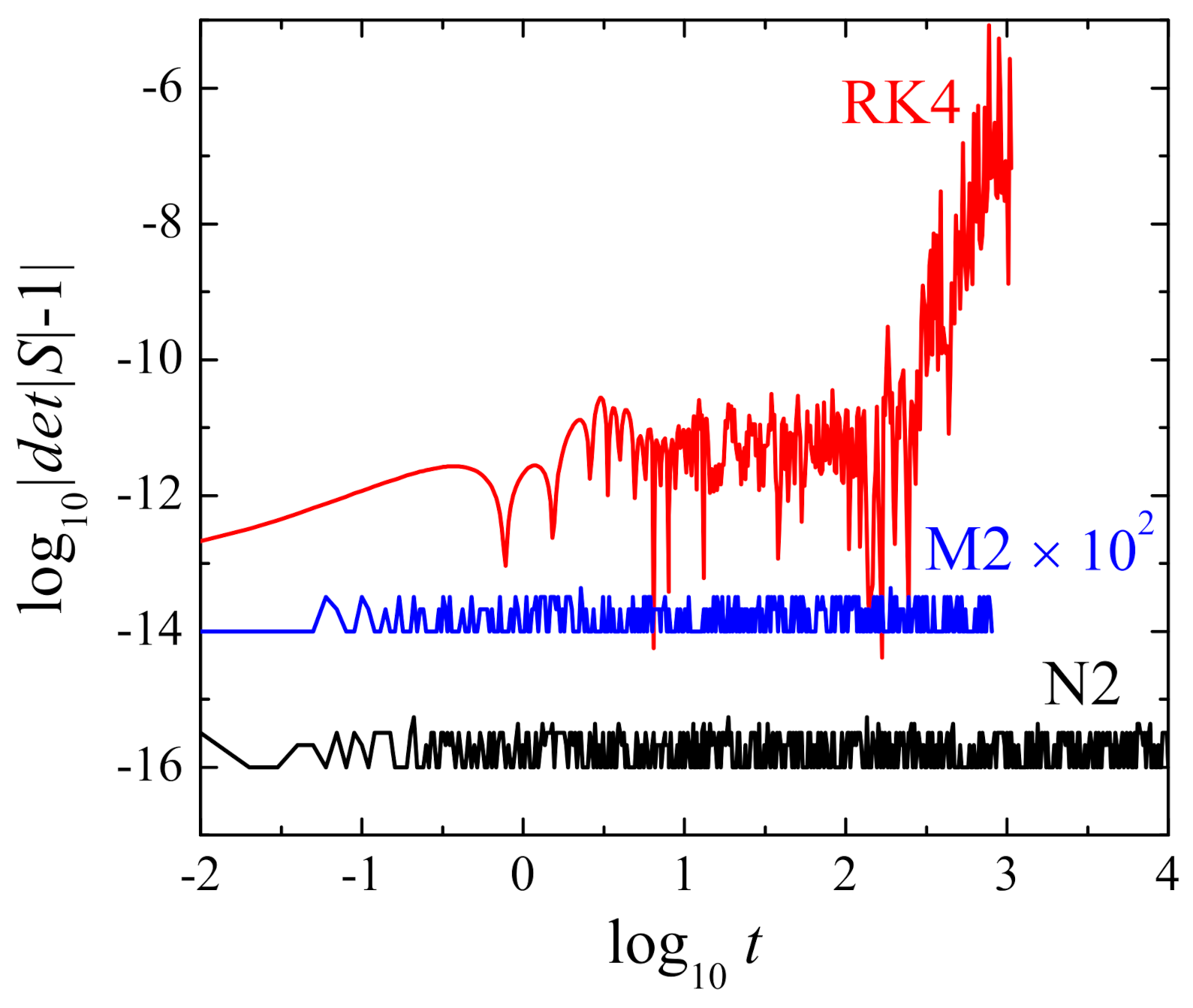
2.3. Preservations of Symplecticity and Volume of the Phase Space

The standard algorithms M2, M4, M4V and M4P are symplectic because A as a Lie operator with respect to the phase flow of a sub-Hamiltonian $H_1=T\left(\mathbf{p}\right)$ is symplectic, and B as a Lie operator with respect to the phase flow of another sub-Hamiltonian $H_2=V\left(\mathbf{q}\right)$ is also symplectic. A product of the two symplectic operators and its compositions are still symplectic for the Hamiltonian (2). That is to say, when operators A and B correspond to the phase flows of the two sub-Hamiltonians for the Hamiltonian (2) (namely, the Hamiltonian (2) is a symplectically separable Hamiltonian system), their composition products are naturally symplectic from a physical point of view [28]. Noting this idea, we can similarly show the symplecticity of the existing force–gradient algorithms (12)–(17) and the extended algorithms (24)–(29). Some discussions are given as follows.

At first, we investigate the construction mechanisms of the existing force–gradient algorithms (12)–(17). As is mentioned above, they are constructed by adding one of the third-order truncation error terms in the second-order method M2 to the potential energy. This is one path for understanding the construction mechanisms of the original force–gradient algorithms. Another path is that the force–gradient algorithms are not directly applied to solve the Hamiltonian (18) but are applied to solve some modified Hamiltonians. To show this, we take a Hamiltonian solved by the algorithm F2 as an example. Equation (12) is a solver of a modified Hamiltonian $H_{\mathrm{F}2}=T+V_{\mathrm{F}2}$, where a modified potential is $V_{\mathrm{F}2}=V\left(\mathbf{q}\right)-\frac{{\tau }^2}{24}{\mathbf{f}}^2$. Operator A acting on the sub-Hamiltonian T advancing a time of $\tau$ is the exact phase flow $e^{\tau A}$ of the sub-Hamiltonian T, and is symplectic. Operator $B_{\mathrm{F}2}=(B+\frac{{\tau }^2}{24}C)$ acting on the sub-Hamiltonian $V_{\mathrm{F}2}$ advancing a time of $\tau /2$ is the exact phase flow $e^{\frac{\tau }{2}{B}_{\mathrm{F}2}}$ of the sub-Hamiltonian $V_{\mathrm{F}2}$, and is also symplectic. Naturally, a composition porduct of these symplectic operators such as $e^{\tau A}{e}^{\frac{\tau }{2}{B}_{\mathrm{F}2}}$ is symplectic [28]. In fact, the explicit symmetric composition scheme F2 for the symplectically separable modified Hamiltonian $H_{\mathrm{F}2}$ is the standard second-order symplectic method M2 with $B\to B_{\mathrm{F}2}$. Of course, different force–gradient symplectic algorithms such as F4 correspond to different modified Hamiltonians. Namely, the force–gradient symplectic algorithms for the original Hamiltonian (2) are the standard symplectic methods for the corresponding modified Hamiltonians.

The construction mechanisms of the extended algorithms (24)–(29) are similar to those of the existing force–gradient algorithms (12)–(17). To show this, we consider the algorithm N2 for the Hamiltonian problem J in Equation (18). There is a modified potential $V_{\mathrm{N}2}\left(\mathbf{q}\right)=V\left(\mathbf{q}\right)-\frac{{\tau }^2}{24}{V}_D\left(\mathbf{q}\right)$, where $V_D\left(\mathbf{q}\right)$ is solved by $\partial V_D\left(\mathbf{q}\right)/\partial q_i={\sum }_{j=1}^n{\sum }_{k=1}^n(2a_{jk}{V}_{q_i{q}_j}{V}_{q_k}+V_{q_j}{V}_{q_k}\frac{\partial a_{jk}}{\partial q_i})$. While the function $V_D$ is difficulty written in general, it should exist from a mathematical point of view. In fact, we do not need to know what the function $V_D$ is, but we need to know only what the function $\partial V_D/\partial q_i$ is. The modified Hamiltonian solved by the algorithm N2 is a symplectically separable Hamiltonian system $J_{N2}=K+V_{\mathrm{N}2}\left(\mathbf{q}\right)$. Only one difference in the construction mechanisms between the force–gradient algorithm F2 and the extended algorithm N2 is that the modified potential $V_{\mathrm{F}2}$ for F2 is easily expressed, whereas the modified potential $V_{\mathrm{N}2}$ for N2 is not. This does not destroy the symplecticity of the algorithm N2 with the extended operator D for the Hamiltonian (18). Similarly, the modified Hamiltonians solved by the algorithms N4 and ${\mathrm{N}4}^{*}$ can be expressed as symplectically separable Hamiltonian systems $J_{\mathrm{N}4}=K+[V\left(\mathbf{q}\right)-\frac{{\tau }^2}{24}(2-\sqrt{3})V_D\left(\mathbf{q}\right)]$ and $J_{{\mathrm{N}4}^{*}}=K+[V\left(\mathbf{q}\right)-\frac{{\tau }^2}{72}{V}_D\left(\mathbf{q}\right)]$. In this way, the symplecticity of the algorithms N4 and ${\mathrm{N}4}^{*}$ is shown sufficiently. The modified Hamiltonians for the extended algorithms (27)–(29) also exist and therefore the extended algorithms remain symplectic.

Precisely speaking, the symplecticity of each of the aforementioned algorithms should satisfy the condition

$$\begin{array}{c}\hfill {\mathbf{S}}^T\mathbf{I}\mathbf{S}=\mathbf{I},\end{array}$$

(30)

where $\mathbf{S}$ and $\mathbf{I}$ are $2n\times 2n$ matrixes. Here, we take four-dimensional phase-space variables $\mathbf{Z}=(x,y,p_x,p_y)$ as an example to show the expressions of $\mathbf{S}$ and $\mathbf{I}$. The solutions ${\mathbf{Z}}_m=(x_m,p_{xm},y_m,p_{ym})$ at an mth step from the solutions ${\mathbf{Z}}_{m-1}=(x_{m-1},p_{xm-1}$, $y_{m-1},p_{ym-1})$ at an $(m-1)$th step advancing the time step $\tau$ for one of the aforementioned algorithms are expressed as

$$\begin{array}{c}\hfill {\mathbf{Z}}_m^T={\mathbf{f}}^T(\tau ,{\mathbf{Z}}_{m-1}),\end{array}$$

(31)

where $\mathbf{f}=(f_x,f_{px},f_y,f_{py})$; that is,

$$\begin{array}{ccc}\hfill x_m& =& f_x(\tau ,x_{m-1},p_{xm-1},y_{m-1},p_{ym-1}),\hfill \\ \hfill p_{xm}& =& f_{px}(\tau ,x_{m-1},p_{xm-1},y_{m-1},p_{ym-1}),\hfill \\ \hfill y_m& =& f_y(\tau ,x_{m-1},p_{xm-1},y_{m-1},p_{ym-1}),\hfill \\ \hfill p_{xm}& =& f_{py}(\tau ,x_{m-1},p_{xm-1},y_{m-1},p_{ym-1}).\hfill \end{array}$$

Their differential forms are $d{\mathbf{Z}}_m^T=\mathbf{S}d{\mathbf{Z}}_{m-1}^T$, where $\mathbf{S}$ is a $4\times 4$ matrix

$$\mathbf{S}=\left(\begin{array}{cccc}\frac{\partial x_m}{\partial x_{m-1}}& \frac{\partial x_m}{\partial y_{m-1}}& \frac{\partial x_m}{\partial p_{xm-1}}& \frac{\partial x_m}{\partial p_{ym-1}}\\ \frac{\partial p_{xm}}{\partial x_{m-1}}& \frac{\partial p_{xm}}{\partial y_{m-1}}& \frac{\partial p_{xm}}{\partial p_{xm-1}}& \frac{\partial p_{xm}}{\partial p_{ym-1}}\\ \frac{\partial y_m}{\partial x_{m-1}}& \frac{\partial y_m}{\partial y_{m-1}}& \frac{\partial y_m}{\partial p_{xm-1}}& \frac{\partial y_m}{\partial p_{ym-1}}\\ \frac{\partial p_{ym}}{\partial x_{m-1}}& \frac{\partial p_{ym}}{\partial y_{m-1}}& \frac{\partial p_{ym}}{\partial p_{xm-1}}& \frac{\partial p_{ym}}{\partial p_{ym-1}}\end{array}\right).$$

(32)

$\mathbf{I}$ is another $4\times 4$ matrix

$$\mathbf{I}=\left(\begin{array}{cccc}0& 0& 0& -1\\ 0& 0& -1& 0\\ 0& 1& 0& 0\\ 1& 0& 0& 0\end{array}\right).$$

(33)

Matrix $\mathbf{S}$ for satisfying the condition (30) is a symplectic matrix. Such symplectic matrixes are present for the above algorithms M2, ⋯, F2, ⋯, N2, ⋯. This symplecticity means a symplectic structure described by a closed nondegenerate differential 2-form $\omega =dx\wedge d{p}_x+dy\wedge d{p}_y$ on a four-dimensional differential manifold ${\mathrm{M}}_4$ (symbol ∧ denotes a wedge product). The condition (30) corresponds to the equality of the symplectic structure ${\omega }_{m-1}$ at the $(m-1)$th step and the symplectic structure ${\omega }_m$ at the mth step: ${\omega }_m={\omega }_{m-1}$. A differential 4-form comes from the product of original differential 2-forms: $\tilde{\omega }=dx\wedge d{p}_x\wedge dy\wedge d{p}_y$. The preservation of differential 2-form naturally leads to that of differential 4-form

$$\begin{array}{c}\hfill {\tilde{\omega }}_m=det\left|\mathbf{S}\right|{\tilde{\omega }}_{m-1},\end{array}$$

(34)

where the determinant of the matrix $\mathbf{S}$ is $det\left|\mathbf{S}\right|=1$. From a geometric point of view, the differential 4-form corresponds to a volume of the phase space:

$$\begin{array}{ccc}& & Vol=|{\tilde{\omega }}_m|=|det\left|\mathbf{S}\right||·|{\tilde{\omega }}_{m-1}|.\hfill \end{array}$$

(35)

Therefore, the differential 4-form and volume of the phase space are preserved when $det\left|\mathbf{S}\right|=1$ (see [28] for more details on the symplectic structure and volume of the phase space). The result on $det\left|\mathbf{S}\right|=1$ will be tested in later numerical experiments.

In short, the novel contribution of this paper is to extend the existing force–gradient symplectic algorithms for the Hamiltonian (2) in [21,22,23] to solve the Hamiltonian (18). Above all, the force–gradient operator C must be replaced by the new operator D.

3. Numerical Simulations

A modified Hénon–Heiles system and a spring pendulum are taken as two models to check the numerical performance of the extended algorithms N4, N4O, N4V and N4P in accuracies of energy and position. Methods M4, M4V and M4P are compared with the extended algorithms. Possible regular and chaotic dynamical differences between the algorithms N4 and M4 are shown. Dynamical behavior of order and chaos in the two problems are described in terms of the best extended algorithm.

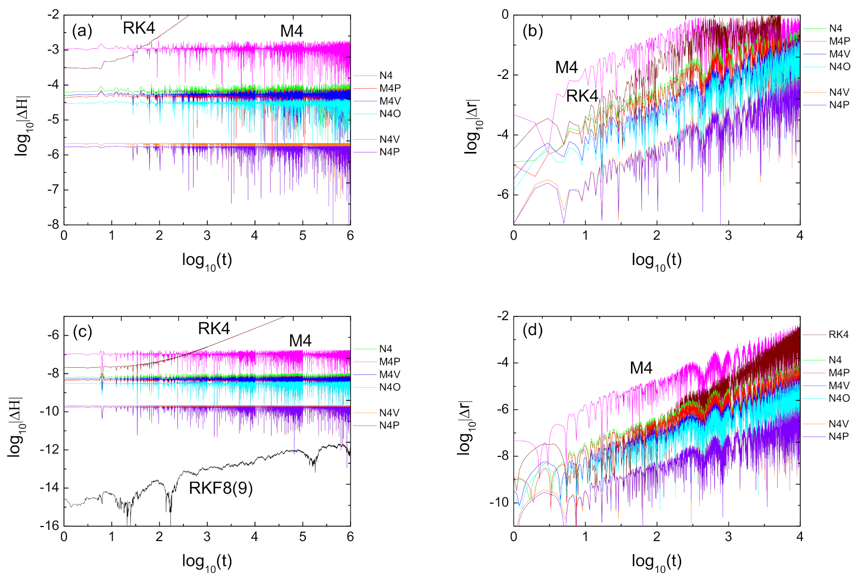
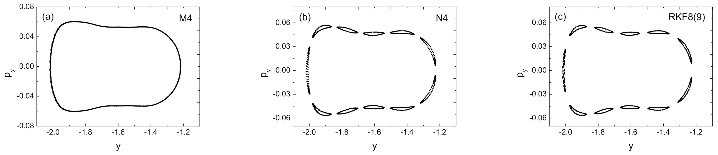
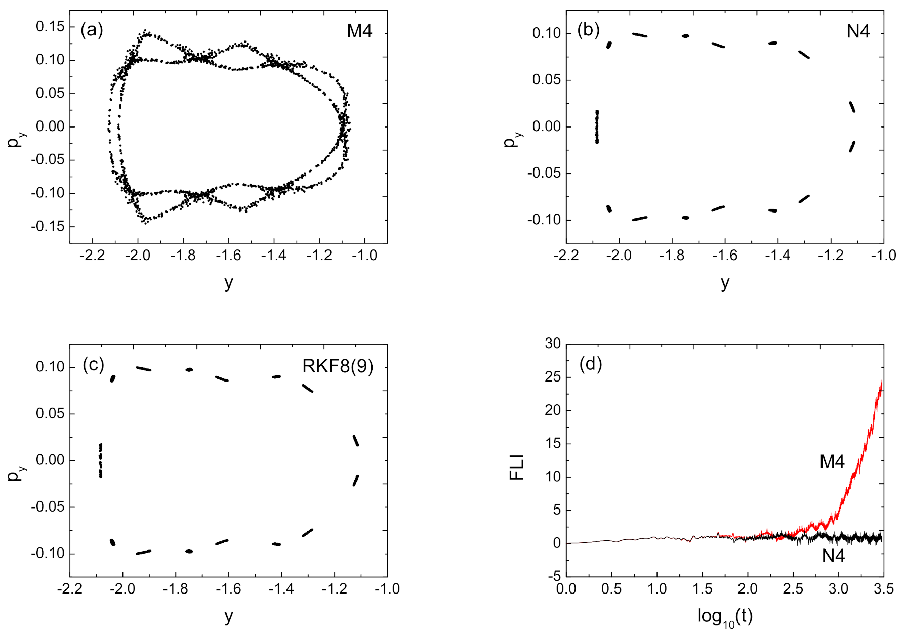
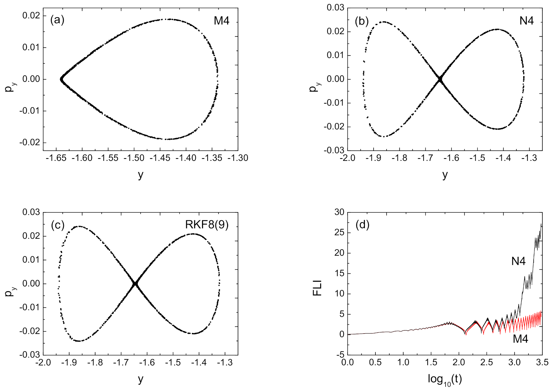
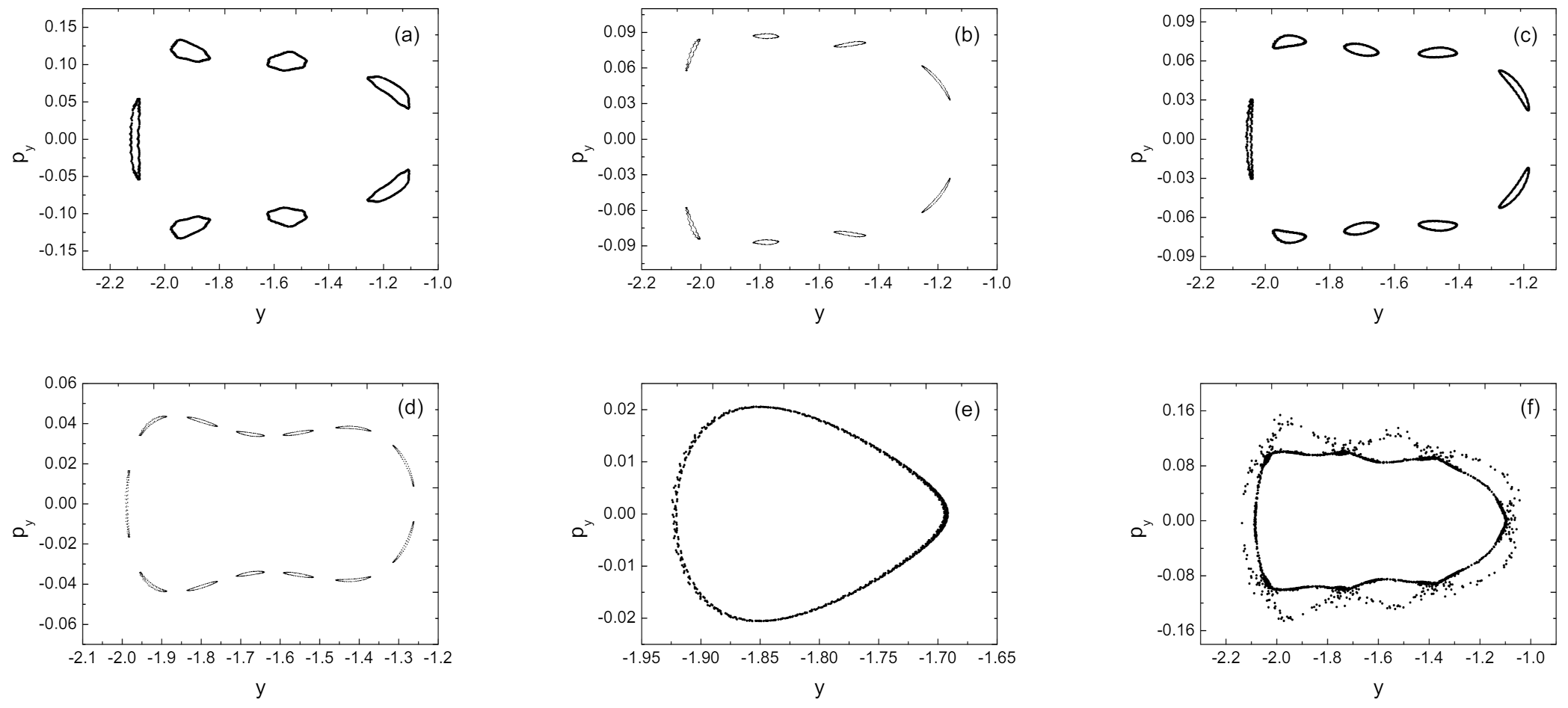
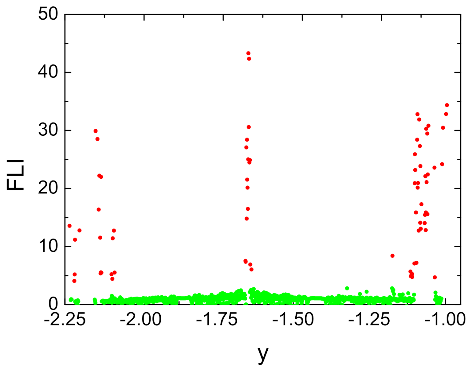
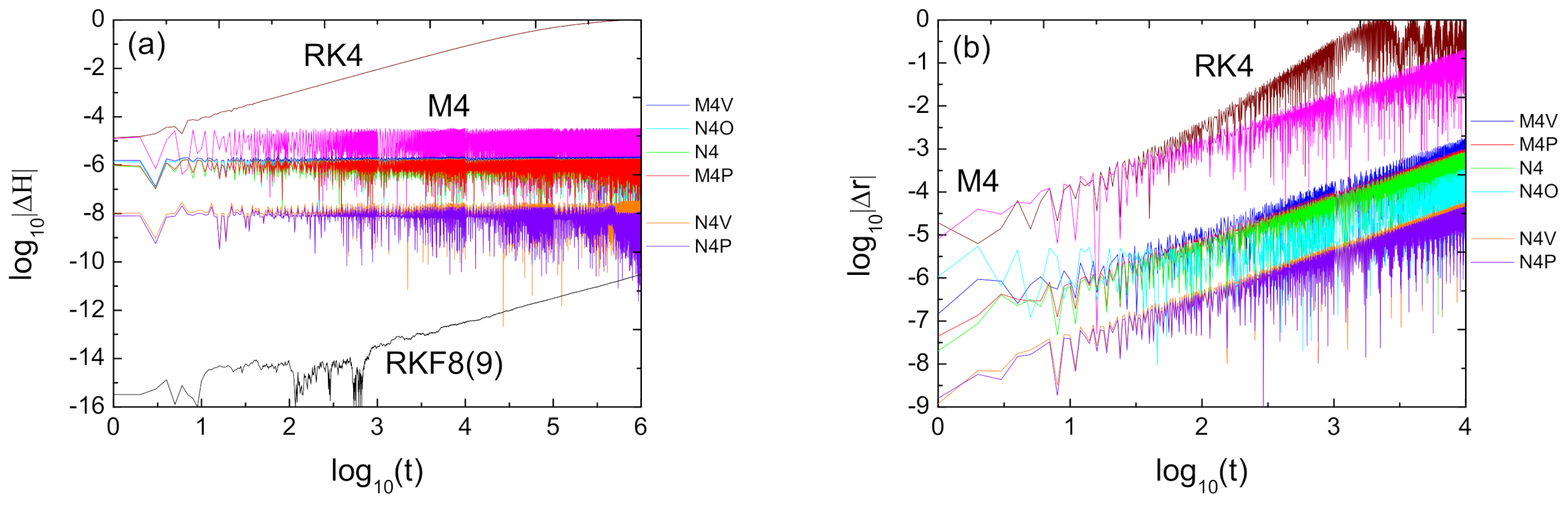
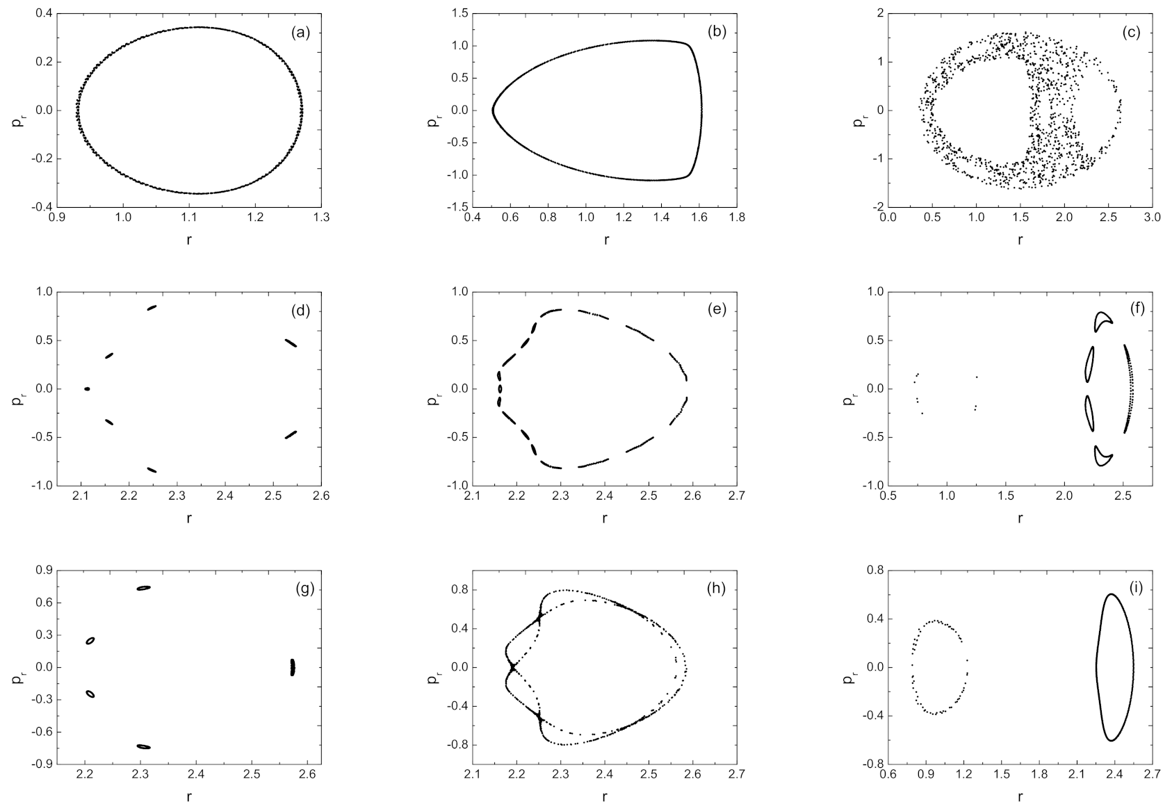
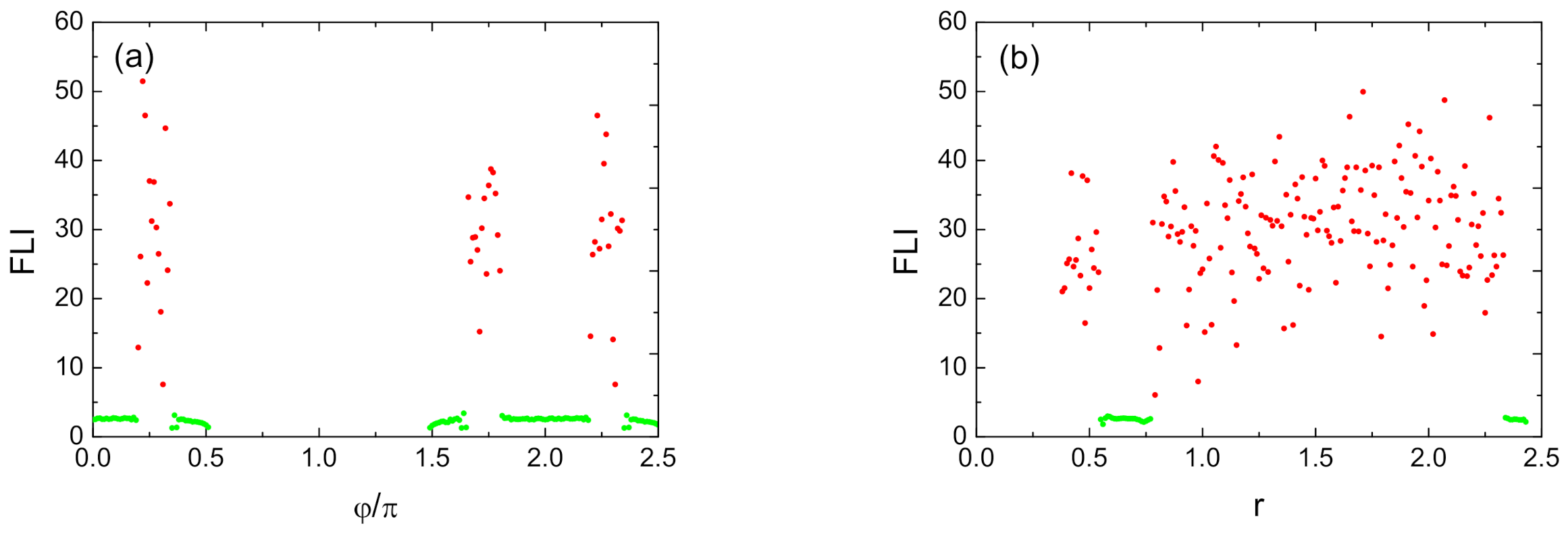
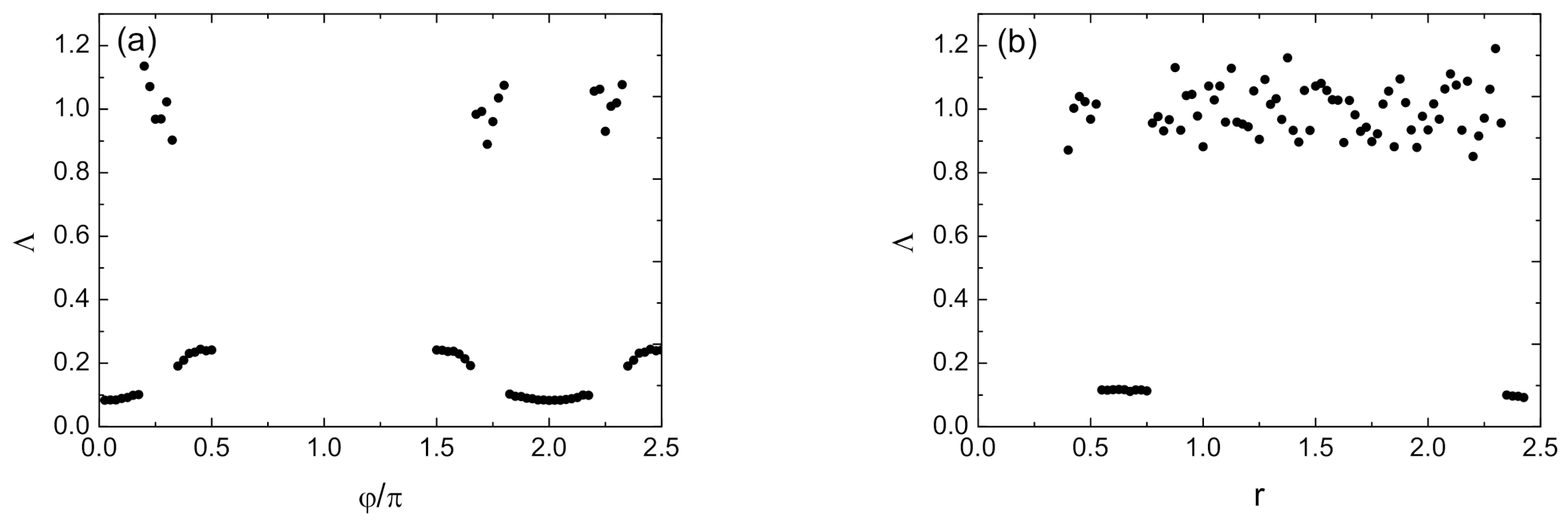
3.1. Modified Hénon–Heiles System

Let us consider a modified Hénon–Heiles system. Set V as the potential of Hénon–Heiles system [29]

$$\begin{array}{c}\hfill V=\frac{1}{2}\left(x^2+y^2\right)+x^{2}y-\frac{1}{3}{y}^3.\end{array}$$

(36)

The standard kinetic energy of Hénon–Heiles system is $T=\left(p_x^2+p_y^2\right)/2$. Here, it is slightly modified as

$$\begin{array}{c}\hfill K=\frac{1}{2}\left(y{p}_x^2+p_y^2\right).\end{array}$$

(37)

K belongs to one of the forms given in Equation (19). Obviously, the operator A for K, the operator B for V and the operator D are easily, analytically solvable. Thus, the algorithms N4, $\mathrm{N}{4}^{*}$, N4O, N4V, N4P, M4, M4V and M4P are easily available for the system $H=K+V$ (for convenience, J in Equation (18) is replaced by H).

The time step is $\tau =0.1$. Energy in the system is $E=1/120$. Initial conditions are $x=0$, $y=-2.02$ and $p_y=0$. The initial positive value of $p_x$ is determined by $E=H$. Figure 1a plots energy errors $|\Delta H|=E_t-E$ for several algorithms, where $E_t$ denotes the numerical energy at time t. The errors have secular growth for the conventional fourth-order Runge–Kutta (RK4), whereas do not have for the algorithms N4, N4O, N4V, N4P, M4, M4V and M4P. The property without secular drift in the energy errors is due to the symplecticity of these methods. The symplectic methods according to the energy errors listed in

Table 1. Energy errors for the algorithms in Figure 1a,c. Because RKF8(9) uses variable time steps, $\tau$ = 0.1 and 0.01 are not time steps but are time intervals for outputting data. Note that 1.29 denotes the error with an order of ${10}^{1.29}$, −9.69 means the error with an order of ${10}^{-9.69}$, and so on.

Method	RK4	RKF8(9)	M4	M4P	M4V	N4	N4O	N4P	N4V
$\tau =0.1$	1.29	−9.69	−2.73	−4.08	−4.13	−3.96	−4.40	−5.75	−5.66
$\tau =0.01$	−3.63	−11.67	−6.75	−8.09	−8.14	−7.97	−8.40	−9.72	−9.67

are mainly divided into three groups as follows. M4 has the poorest anergy accuracy, and N4P and N4V have the best anergy accuracies. N4P and N4V have almost the same accuracy, and their accuracies are about three orders of magnitude better than the accuracy for M4. The four methods N4, M4P, M4V and N4O have minor differences in the energy accuracies. The errors for large to small are N4, M4P, M4V and N4O. In particular, the accuracy for N4 is one order of magnitude better than that for M4. A position error at time t for each of the methods RK4, N4, N4O, N4V, N4P, M4, M4V and M4P is estimated by $|\Delta \mathbf{r}|=\sqrt{{(x_2-x_1)}^2+{(y_2-y_1)}^2}$, where the solutions $(x_1,y_1)$ are given by the method, and the solutions $(x_2,y_2)$ are obtained from the higher-precision integrator RKF8(9). When the integration time reaches ${10}^4$ corresponding to ${10}^5$ steps, the position errors are shown in Figure 1b and

Table 2. Position errors for the algorithms in Figure 1b,d.

Method	RK4	M4	M4P	M4V	N4	N4O	N4P	N4V
$\tau =0.1$	0.47	0.006	−0.56	−0.63	−0.49	−0.87	−2.06	−2.03
$\tau =0.01$	−2.38	−2.32	−4.07	−4.50	−3.96	−4.72	−5.858	−5.856

. RK4 has the largest error with an order of ${10}^{0.47}$. The position error for M4 is also larger than 1. The position errors for N4P and N4V are two orders of magnitude smaller than that for M4, and one order of magnitude smaller than those for the four methods N4, M4P, M4V and N4O. The four methods N4, M4P, M4V and N4O are almost the same in the position errors. These results in Table 1 and Table 2 indicate that the standard symplectic integrators without the operator D are poorer than the corresponding extended methods with the operator D in energy accuracies (e.g., M4 inferior to N4, M4V and M4P inferior to N4O, N4V and N4P). The optimized methods are better than the corresponding non-optimized methods (e.g., M4V and M4P superior to M4, and N4O, N4V and N4P superior to N4). The optimized methods with one free coefficient are inferior to those with two free coefficients (e.g., N4O inferior to N4V and N4P). Clearly, M4 performs the poorest accuracy, and N4V and N4P exhibit the best accuracies.

The smaller the time step gets, the higher the accuracy of an integrator is. When the time step is appropriately smaller, e.g., $\tau =0.01$, the energy errors are described in Figure 1c and Table 1. The errors are ${10}^{-6.75}$ for M4, ${10}^{-8}$ for N4, M4V, M4P, and N4O, and ${10}^{-9.7}$ for N4V and N4P. That is, the energy errors typically decrease for each symplectic algorithm. While RKF8(9) as a non-symplectic method has a secular drift in the energy errors, it has the best energy accuracy and is a good reference integrator for evaluating the performance of the other methods. The position errors in Figure 1d and Table 2 are about ${10}^{-2}$ for M4 and RK4, ${10}^{-5}$∼${10}^{-4}$ for M4V, M4P, N4 and N4O, and ${10}^{-6}$ for N4V and N4P. That is to say, as far as the accuracies of energy and position for the smaller time step $\tau =0.01$ are concerned, M4 is still the poorest one, and N4V and N4P are the best ones among the symplectic methods.

Table 3. CPU times (unit: Second) of each algorithm in Figure 1a,c.

Method	RK4	RKF8(9)	M4	M4P	M4V	N4	N4O	N4P	N4V
$\tau =0.1$	0.33	24	0.51	0.66	0.64	0.44	0.44	0.59	0.59
$\tau =0.01$	2.56	83	4.53	5.89	5.70	3.63	3.64	5.22	5.23

lists CPU times for each algorithm in Figure 1a,c. RK4 is the fastest, and RKF8(9) is the slowest. The computational efficiencies of the symplectic integrators from high to low are N4, N4O, M4, N4P, N4V, M4V and M4P. Of course, there are no relatively dramatic differences in the computational cost between N4 (or N4O) and N4P (or N4V).

Figure 2 is used to check whether the determinants of the matrix $\mathbf{S}$, $det\left|\mathbf{S}\right|$, are 1 for the three methods RK4, M2 and N2. The error $det\left|\mathbf{S}\right|-1$ for RK4 grows with time spanning 300. This means that RK4 does not satisfy Equations (34) and (35). However, the errors $det\left|\mathbf{S}\right|-1$ for M2 and N2 almost remain at the machine precision in the double-precision environment. This sufficiently supports the preservations of the differential 4-form $\tilde{\omega }$ and the phase-space volume in the standard symplectic method M2 and the extended algorithm N2. In principle, $det\left|\mathbf{S}\right|\ne 1$ for RKF8(9) and $det\left|\mathbf{S}\right|=1$ for the fourth-order methods M4, M4V, M4P, N4, N4${}^{*}$, N4O, N4V and N4P can be confirmed numerically. However, the matrixes $\mathbf{S}$ for these algorithms have such long expressions (with over 1000 pages outputted by Matlab) that their determinants are difficultly computed.

Figure 3 shows that the two symplectic integrators N4 and M4 provide different dynamical phase-space structures to the same orbit in Figure 1 because they have different numerical accuracies for the time step $\tau =0.1$. A single Kolmogorov-Arnold-Moser (KAM) torus on the Poincaré section $x=0$ with $p_x>0$ is described by the Forest-Ruth method M4 in Figure 3a, but many islands are given by the newly extended method N4 in Figure 3b. While the two tori are regular, they are different. In fact, a many-islands torus becomes easier for the occurrence of chaos than a single torus. Which of the algorithms M4 and N4 can provide correct results? N4 can because the results of N4 are consistent with those of higher-precision method RKF8(9) in Figure 3c, and are also the same as those of the five methods M4V, M4P, N4O, N4V and N4P. The different KAM tori described by the two methods N4 and M4 are because N4 is one order of magnitude better than M4 in the accuracies of energy and position, as shown in Figure 1a,b. In other words, the time step $\tau =0.1$ is too large to be chosen for M4. However, the phase-space structures can be truly described by M4 for the smaller time step $\tau =0.01$ because M4 has better accuracies for the smaller time step $\tau =0.01$ than for the larger time step $\tau =0.1$ (see Figure 1 and Table 1 and Table 2 for more information).

Only when the initial value $y=-1.108$ with the initial value $p_x$ is altered, does M4 with the larger time step $\tau =0.1$ indicate that the orbit considered in Figure 4a seems to be a many-islands torus, but exhibits the chaoticity because many discrete points are randomly filled with small regions. Unlike M4, N4 with the larger time step $\tau =0.1$ and RKF8(9) show the regularity of the same orbit in Figure 4b,c. As claimed above, N4 is superior to M4 in accuracy; therefore, the KAM torus is physically given by N4, but the non-physically spurious chaoticity is caused by M4. These results are also confirmed by fast Lyapunov indicators (FLIs) in Figure 4d. The FLIs are from a modified form of Lyapunov exponents [30]. They are originally defined in terms of the lengths of tangent vectors by Froeschlé & Lega [31]. Using the phase-space distances between two adjacent orbits at times 0 and t, $d\left(0\right)$ and $d\left(t\right)$, Wu et al. [32] suggested the computation of FLI according to the following form

$$\mathrm{FLI}={log}_{10}\frac{d\left(t\right)}{d\left(0\right)}.$$

(38)

A bounded orbit is ordered if its FLI grows algebraically with time ${log}_{10}t$, but chaotic when its FLI increases exponentially. In other words, the method of complete different growth rates of FLIs with time is faster to distinguish between the two cases of order and chaos than the technique of Lyapunov exponents. When the integration time reaches 3000 in Figure 4d, the FLI is 25 for M4, and smaller than 2.5 for N4. Clearly, M4 and N4 for the larger time step $\tau =0.1$ indeed give the orbit chaotic and regular dynamical behaviors, respectively. Of course, the chaoticity for M4 is spurious because of M4 performing the poor accuracy. If the smaller time step $\tau =0.01$ is adopted, M4 like N4 can give the true dynamical behavior to the orbit.

Given the initial value $y=-1.654$ and the larger time step $\tau =0.1$, the methods of Poincaré section and FLI in Figure 5 show that the integrated orbit is a regular single torus for M4, whereas a figure-eight orbit for N4 and RKF8(9). The figure-eight orbit seems to be regular, but is in fact chaotic due to the existence of a hyperbolic point, which has a stable direction and a unstable direction. The chaoticity for N4 is physical, but the regular dynamical information given by M4 is not physical. This is because M4 does not give high enough accuracy to the numerical solutions, but N4 does. M4 can also provide the reliable results for the smaller time step $\tau =0.01$. In addition, the energy error (not plotted) of the chaotic orbit for N4 in Figure 5 is similar to that of the regular orbit for N4 in Figure 1. Namely, the energy accuracy for N4 is independent of the regularity or chaoticity of orbits.

Several main results can be concluded from the above demonstrations. The standard symplectic integrators without the operator D are inferior to the corresponding extended methods with the operator D in computational accuracies and efficiencies. The optimized methods have better accuracies than the corresponding non-optimized methods. N4V and N4P exhibit the best accuracies. While N4 can provide reliable results on the orbital dynamical behavior for the larger time step $\tau =0.1$, one of the two optimized extended methods N4P and N4V should be the best integrator from the computational accuracies and efficiencies.

Now, we apply the optimized extended method N4P with the large time step $\tau =0.1$ to explore the dynamics of the modified Hénon–Heiles system. As the magnitude of negative initial value of y decreases, there is a dynamical transition from physical many-islands tori (Figure 6a–d), to single torus (Figure 6e) and to chaotic orbits (Figure 6f). This seems to show that the strength of chaos is enhanced with a decrease of the magnitude of negative initial value of y. However, chaos is not always enhanced, as can be seen from the dependence of FLI on the initial value of y in Figure 7 that displays the dynamical transition from order to chaos. Chaos mainly occurs for the initial values of y in the vicinity of −2.25∼−2.1, −1.6, and −1.2∼−1. Here, the initial value $x=0$ is fixed, and each value of FLI is obtained after integration time $t=3000$. Numerical tests show that the threshold of FLIs between the ordered and chaotic cases is 4. The FLIs larger than the threshold determine the chaoticity of bounded orbits, but the FLIs less than the threshold indicate the regularity of bounded orbits.

3.2. Spring Pendulum

A spring pendulum in polar coordinates is described by the Hamiltonian [1]

$$\begin{array}{c}\hfill H=\frac{1}{2}\left(p_r^2+\frac{p_{\phi }^2}{r^2}\right)-rcos\phi +{(r-1)}^2.\end{array}$$

(39)

The Hamiltonian is divided into kinetic energy K and potential energy V as follows:

$$\begin{array}{ccc}\hfill K& =& \frac{1}{2}\left(p_r^2+\frac{p_{\phi }^2}{r^2}\right),\hfill \end{array}$$

(40)

$$\begin{array}{ccc}\hfill V& =& -rcos\phi +{(r-1)}^2.\hfill \end{array}$$

(41)

K is one of the expressions in Equation (19) and is analytically solved. In this case, the extended algorithms such as N4 can be suitable for integrating the spring pendulum problem.

Taking the step size $\tau =0.1$ and energy $E=1/12$, we choose initial conditions $r=1.15$, $p_r=0$ and $\phi =0.05\pi$. The initial value $p_{\phi }>0$ is solved from the energy equation $E=H$. Figure 8 and

Table 4. Energy errors $|\Delta H|$ and position errors $|\Delta r|$ for the algorithms in Figure 8.

Method	RK4	RKF8(9)	M4	M4P	M4V	N4	N4O	N4P	N4V
$|\Delta H|$	0.04	−10.53	−4.47	−5.73	−5.65	−5.73	−5.74	−7.65	−7.47
$|\Delta r|$	0.13		−0.67	−2.99	−2.74	−3.06	−3.45	−4.34	−4.24

show that RK4 has the largest errors in the energy and position, and RKF8(9) exhibits the smallest energy error. The errors in the energy have secular drifts for the non-symplectic methods RK4 and RKF8(9), but do not have for the symplectic methods M4, M4V, M4P, N4, N4O, N4V and N4P. The errors in the energy and position for N4V and N4P are about three orders of magnitude smaller than those for M4.

Table 5. CPU times (unit: second) of each algorithm in Figure 8a.

Method	RK4	RKF8(9)	M4	M4P	M4V	N4	N4O	N4P	N4V
Time	0.73	28	3.70	4.56	3.86	2.78	2.98	3.89	3.30

lists CPU times of the methods. The standard symplectic methods are slower than the corresponding extended schemes in computational efficiencies. The optimized methods N4V and N4P need small additional cost compared with the corresponding non-optimized method N4.

The tested orbit in Figure 8 is a regular single closed torus on the Poincaré section $\phi =0$ and $p_{\phi }>0$ in Figure 9a. Unlike in the modified Hénon–Heiles system, M4 in the present problem is the same as anyone of the methods M4V, M4P, N4, N4O, N4V, N4P and RKF8(9) in the description of phase-space structures. This is because the accuracies in the energy and position for M4 in Figure 8 are higher than those in Figure 1. In fact, the energy for M4 is accurate to an order of ${10}^{-3}$, and the position for M4 is accurate to an order of 1 in Figure 1 when the integration time $t={10}^4$. However, the energy for M4 is accurate to an order of ${10}^{-5}$, and the position for M4 is accurate to an order of 0.1 in Figure 8 when the integration time $t={10}^4$. Because of this, M4 can truly describe the phase-space structures, as the methods M4V, M4P, N4, N4O, N4V, N4P and RKF8(9) can. For given integrator and time step, the numerical accuracy closely depends on model Hamiltonians, and particularly depends on the periods of orbits in the Hamiltonians. The larger the periods are, the better the numerical accuracy is.

Considering the best performance in numerical accuracies and computational efficiency, we use N4P to trace different phase-space structures when various initial values are given to $\phi$. For example, single-torus orbits exist for $\phi =0.19\pi$ in Figure 9b and $\phi =0.358\pi$ in Figure 9e. There are many islands for $\phi =0.35\pi$ in Figure 9d, $\phi =0.361\pi$ in Figure 9f, $\phi =0.366\pi$ in Figure 9g, and $\phi =0.39\pi$ in Figure 9i. Chaos occurs for $\phi =0.2\pi$ in Figure 9c and $0.376\pi$ in Figure 9h. No universal rule for the dynamical transition from order to chaos seems to be given to a variation of the initial value $\phi$. However, Figure 10a for the description of the initial values of $\phi$ and their corresponding FLIs shows that chaos mainly occurs for the initial values of $\phi$ in the vicinity of 0.25, 1.75, and 2.25. This is because the spring pendulum suffers from strong perturbations in the vicinity of $\phi =\pi /4,7\pi /4$. Scanning the initial values of r and their corresponding FLIs in Figure 10b displays that chaos mainly occurs for the initial values of r in the vicinity of 0.5, and 0.75∼2.25.

Besides the method of FLIs, the 0–1 test for chaos [33] can be applied to explore the transition from order to chaos with the initial value $\phi$ or r varying. The 0–1 test chaos indicator is described here. Set $\mathbf{Z}=(r,\phi ,p_r,p_{\phi })$ as a solution of the system (39) at time t. $\psi \left(\mathbf{Z}\right)$ is a function of $\mathbf{Z}$; for example, $\psi \left(\mathbf{Z}\right)=r$ is a simple choice. The authors of [33] defined two functions

$$\begin{array}{ccc}\hfill \theta \left(t\right)& =& ct+{\int }_0^t\psi \left(\mathbf{Z}\left(s\right)\right)ds,\hfill \end{array}$$

(42)

$$\begin{array}{ccc}\hfill q\left(t\right)& =& {\int }_0^t\psi \left(\mathbf{Z}\left(s\right)\right)cos\left(\theta \left(s\right)\right)ds,\hfill \end{array}$$

(43)

where $c>0$ is an arbitrarily constant. The mean-square displacement of $q\left(t\right)$ is

$$\begin{array}{c}\hfill L\left(t\right)=\underset{T\to \infty }{lim}\frac{1}{T}{\int }_0^T{[q(t+s)-q\left(s\right)]}^2\mathrm{d}s.\end{array}$$

(44)

Finally, the asymptotic growth rate of the mean-square displacement is expressed as

$$\begin{array}{c}\hfill \Lambda =\underset{t\to \infty }{lim}\frac{lnL\left(t\right)}{lnt}.\end{array}$$

(45)

Based on ergodic theory, $\Lambda =0$ signifies regular dynamics, but $\Lambda =1$ signifies chaotic dynamics. Taking $c=1.8$, $T=$ 1,000,000, $t=1000$ and time step $\tau =0.1$, we calculate the values of $\Lambda$ with respect to the orbits in Figure 10 and obtain the dependence of $\Lambda$ on the initial values $\phi$ in Figure 11. The values of $\Lambda$ in Figure 11a are in the vicinity of 1 when the initial values of $\phi$ are in the vicinity of 0.25, 1.75 and 2.25, and are in the vicinity of 0 when the initial values of $\phi$ are in the vicinity of 0.1, 0.5, 1.5, 2.0 and 2.5. The values of $\Lambda$ in Figure 11b are in the vicinity of 1 when the initial values of r are in the vicinity of 0.5, and 0.75∼2.25, and are in the vicinity of 0 when the initial values of r are in the vicinity of 0.7 and 2.5. That is to say, the dynamical properties described by the 0–1 indicator $\Lambda$ in Figure 11 are consistent with those given by the FLIs in Figure 10. However, because T is large enough, computations of $L\left(t\right)$ are relatively expensive. In fact, CPU time is 284.41 s for each of the $\Lambda$ values in Figure 11, and 0.36 s for each of the FLIs in Figure 10. Thus, the FLIs are quicker to distinguish between the ordered and chaotic two cases than the 0–1 test indicator.

4. Conclusions and Discussions

Many force–gradient explicit symplectic integration algorithms with the force–gradient operator C for the Hamiltonian (2) with the kinetic energy (1) have been in [21,22,23]. However, these algorithms become useless for the Hamiltonian (18) with the integrable kinetic energy (19) if the force–gradient operator C is not altered. We find that the existing integrators are still available for the Hamiltonian (18) when the force–gradient operator C gives place to a new operator D. This new operator is not a force–gradient operator but is similar to the momentum-version operator associated to the potential V. The extended algorithms are no longer solvers of the original Hamiltonian but are solvers of slightly modified Hamiltonians. They are explicit symplectic integrators with symmetry or time reversibility.

Numerical tests show that the standard symplectic integrators without the operator D are generally inferior to the corresponding extended methods with the operator D in computational accuracies and efficiencies. For example, the fourth-order Forest-Ruth symplectic scheme cannot provide reliable results to the description of regular and chaotic dynamical features of the modified Hénon–Heiles system for the use of some appropriately large time steps, but the corresponding extended ones can. The optimized methods have better accuracies than the corresponding non-optimized methods. Among the tested symplectic methods, the two extended optimized seven-stage fourth-order methods of Omelyan, Mryglod and Folk (N4V and N4P) exhibit the best numerical performance, and their accuracies are about three orders of magnitude better than the accuracies of the Forest-Ruth symplectic scheme. Finally, one of the two optimized algorithms is used to study the orbital dynamical features of the modified Hénon–Heiles system and the spring pendulum.

The proposed extended algorithms are suitably applicable to any Hamiltonian systems like the Hamiltonian system (18). The kinetic energies like Equation (19) can be found in some references. For example, the Hamiltonian in Equation (5.21) of [34] is

$$H=\frac{1}{2}(p_1^2+p_2^2)+\frac{\epsilon }{2}{p}_1^{2}cos{x}_2+cos{x}_1-1.$$

(46)

The kinetic energies given in Equation (40) are universal for two-dimensional Hamiltonian systems $H=m({\dot{x}}^2+{\dot{y}}^2)/2+V(x,y)$ in polar coordinates $(r,\phi )$, where potentials $V(x,y)$ are non-axisymmetric. In addition, three-dimensional Hamiltonian problems $H=m({\dot{x}}^2+{\dot{y}}^2+{\dot{z}}^2)/2+V(x,y,z)$ in spherical coordinates $(r,\theta ,\phi )$ are expressed as

$$H=\frac{1}{2m}(p_r^2+\frac{p_{\theta }^2}{r^2}+\frac{p_{\phi }^2}{r^2{sin}^2\theta })+V(r,\theta ,\phi ),$$

(47)

which resembles the Hamiltonian (18) with the integrable kinetic energy (19). In other words, the Hamiltonian (18) is not restricted to several special examples, but is often met in many situations. In this sense, this extension has wide applications. As an example, the kinetic energies in the Hamiltonians of the spiral structure in self-consistent models of rotating galaxies [35] and the spiral arms in galaxies [36] are Equation (40). Thus, the newly extended force–gradient explicit symplectic methods should be suitable for the study of chaotic spiral arms in the models of rotating galaxies. This problem will be considered in future work.

References

1. Hairer, E.; Lubich, C.; Wanner, G. Geometric Numerical Integration: Structure-Preserving Algorithms for Ordinary Differential Equations, 2nd ed.; Springer: Berlin/Heidelberg, Germany, 2006. [Google Scholar]
2. Wisdom, J. The origin of the Kirkwood gaps—A mapping for asteroidal motion near the 3/1 commensurability. Astron. J. 1982, 87, 577. [Google Scholar] [CrossRef]
3. Ruth, R.D. A Canonical Integration Technique. IEEE Trans. Nucl. Sci. 1983, 30, 2669. [Google Scholar] [CrossRef]
4. Feng, K. On difference schemes and symplectic geometry. In Proceedings of the 1984 Beijing Symposium on Differential Geometry and Differential Equations; Feng, K., Ed.; Science Press: Beijing, China, 1985; p. 42. [Google Scholar]
5. Nacozy, P.E. The Use of Integrals in Numerical Integrations of the N-Body Problem. Astrophys. Space Sci. 1971, 14, 40. [Google Scholar] [CrossRef]
6. Fukushima, T. Efficient Orbit Integration by Scaling for Kepler Energy Consistency. Astron. J. 2003, 126, 1097. [Google Scholar] [CrossRef] [Green Version]
7. Bacchini, F.; Ripperda, B.; Chen, A.Y.; Sironi, L. Generalized, Energy-conserving Numerical Simulations of Particles in General Relativity. I. Time-like and Null Geodesics. Astropys. J. Suppl. 2018, 237, 6. [Google Scholar] [CrossRef] [Green Version]
8. Feng, K.; Qin, M. The symplectic methods for the computation of hamiltonian equations. Lect. Note Math. 1987, 1297, 1. [Google Scholar]
9. Sanz-Serna, J.M. Runge-kutta schemes for Hamiltonian systems. BIT 1988, 28, 877. [Google Scholar] [CrossRef]
10. Kopáček, O.; Karas, V.; Kovář, J.; Stuchlík, Z. Transition from Regular to Chaotic Circulation in Magnetized Coronae near Compact Objects. Astrophys. J. 2010, 722, 1240. [Google Scholar] [CrossRef]
11. Liao, X.H. Symplectic Integrator for General Near-Integrable Hamiltonian System. Celest. Mech. Dyn. Astron. 1997, 66, 243. [Google Scholar] [CrossRef]
12. Preto, M.; Saha, P. On Post-Newtonian Orbits and the Galactic-center Stars. Astrophys. J. 2009, 703, 1743. [Google Scholar] [CrossRef] [Green Version]
13. Lubich, C.; Walther, B.; Brügmann, B. Symplectic integration of post-Newtonian equations of motion with spin. Phys. Rev. D 2010, 81, 104025. [Google Scholar] [CrossRef] [Green Version]
14. Forest, E. Geometric integration for particle accelerators. J. Phys. A Math. Gen. 2006, 39, 5321. [Google Scholar] [CrossRef]
15. Wang, Y.; Sun, W.; Liu, F.; Wu, X. Construction of Explicit Symplectic Integrators in General Relativity. I. Schwarzschild Black Holes. Astrophys. J. 2021, 907, 66. [Google Scholar] [CrossRef]
16. Pihajoki, P. Explicit methods in extended phase space for inseparable Hamiltonian problems. Celest. Mech. Dyn. Astron. 2015, 121, 211. [Google Scholar] [CrossRef] [Green Version]
17. Forest, E.; Ruth, R. Fourth-order symplectic integration. Phys. D 1990, 43, 105. [Google Scholar] [CrossRef] [Green Version]
18. Yoshida, H. Construction of higher order symplectic integrators. Phys. Lett. A 1990, 150, 262. [Google Scholar] [CrossRef]
19. Suzuki, M.; Umeno, K. Computer Simulation Studies in Condensed Matter Physics VI; Landau, D.P., Mon, K.K., Schüttler, H.-B., Eds.; Springer: Berlin/Heidelberg, Germany, 1993. [Google Scholar]
20. Omelyan, I.P.; Mryglod, I.M.; Folk, R. Optimized Forest-Ruth- and Suzuki-like algorithms for integration of motion in many-body systems. Comput. Phys. Commun. 2002, 146, 188. [Google Scholar] [CrossRef] [Green Version]
21. Chin, S.A. Symplectic integrators from composite operator factorizations. Phys. Lett. A 1997, 226, 344. [Google Scholar] [CrossRef]
22. Omelyan, I.P.; Mryglod, I.M.; Folk, R. Construction of high-order force–gradient algorithms for integration of motion in classical and quantum systems. Phys. Rev. E 2002, 66, 026701. [Google Scholar] [CrossRef] [Green Version]
23. Omelyan, I.P.; Mryglod, I.M.; Folk, R. Symplectic analytically integrable decomposition algorithms: Classification, derivation, and application to molecular dynamics, quantum and celestial mechanics simulations. Comput. Phys. Commun. 2003, 151, 272. [Google Scholar] [CrossRef]
24. Wisdom, J.; Holman, M. Symplectic maps for the N-body problem. Astron. J. 1991, 102, 1528. [Google Scholar] [CrossRef]
25. Chambers, J.E.; Murison, M.A. Pseudo-High-Order Symplectic Integrators. Astron. J. 2000, 119, 425. [Google Scholar] [CrossRef] [Green Version]
26. Hernandez, D.M.; Dehnen, W. A study of symplectic integrators for planetary system problems: Error analysis and comparisons. Mon. Not. Astron. Soc. 2017, 468, 2614. [Google Scholar] [CrossRef] [Green Version]
27. Swope, W.C.; Andersen, H.C.; Berens, P.H.; Wilson, K.R. A computer simulation method for the calculation of equilibrium constants for the formation of physical clusters of molecules: Application to small water clusters. J. Chem. Phys. 1982, 76, 637. [Google Scholar] [CrossRef]
28. Feng, K.; Qin, M. Symplectic Geometric Algorithms for Hamiltonian Systems, Zhejiang Science and Technology Publishing House: Hangzhou, China; Springer: Berlin/Heidelberg, Germany, 2010. [Google Scholar]
29. Hénon, M.; Heiles, C. The applicability of the third integral of motion: Some numerical experiments. Astron. J. 1964, 69, 73. [Google Scholar] [CrossRef] [Green Version]
30. Tancredi, G.; Sánchez, A.; Roig, F. A Comparison Between Methods to Compute Lyapunov Exponents. Astron. J. 2001, 121, 1171. [Google Scholar] [CrossRef]
31. Froeschlé, C.; Lega, E. On the Structure of Symplectic Mappings. The Fast Lyapunov Indicator: A Very Sensitive Tool. Celest. Mech. Dyn. Astron. 2000, 78, 167. [Google Scholar] [CrossRef]
32. Wu, X.; Huang, T.; Zhang, H. Lyapunov indices with two nearby trajectories in a curved spacetime. Phys. Rew. D. 2006, 74, 083001. [Google Scholar] [CrossRef] [Green Version]
33. Gottwald, G.A.; Melbourne, I. A new test for chaos in deterministic systems. Proc. R. Soc. A Math. Phys. Eng. Sci. 2004, 460, 603. [Google Scholar] [CrossRef] [Green Version]
34. Itoh, T.; Abe, K. Hamiltonian-Conserving Discrete Canonical Equations Based on Variational Difference Quotients. J. Comp. Phys. 1988, 76, 85. [Google Scholar] [CrossRef]
35. Voglis, N.; Stavropoulos, I.; Kalapotharakos, C. Chaotic motion and spiral structure in self-consistent models of rotating galaxies. Mon. Not. R. Astron. Soc. 2006, 372, 901. [Google Scholar] [CrossRef] [Green Version]
36. Harsoula, M.; Efthymiopoulos, C.; Contopoulos, G. Analytical forms of chaotic spiral arms. Mon. Not. R. Astron. Soc. 2016, 459, 748. [Google Scholar] [CrossRef] [Green Version]
Figure 1. (a) Energy errors for several algorithms independently solving the modified Hénon–Heiles system. The time step is τ = 0.1 , and energy is E = 1 / 120 . Initial conditions are x = 0 , y = 2.02 and p y = 0 . The positive initial value of p x is given by the energy relation E = H . (b) Position errors between the solutions of RKF8(9) and the other methods. (c,d) are the same as (a,b) but a smaller time step τ = 0.01 is used. These errors are clearly listed in Table 1 and Table 2.
Mathematics 09 02718 g001
Figure 2. Difference between 1 and the determinant d e t | S | of the matrix S for each of the three methods RK4, M2 and N2. The time step is τ = 0.01 and energy is E = 1 / 120 . The initial conditions are x = 0 , y = 0.988 and p y = 0 . M 2 × 100 means that the plotted values are 100 times larger than the practical values.
Mathematics 09 02718 g002
Figure 3. Poincaré sections at the plane x = 0 and p x > 0 . The Poincaré sections in (a), (b) and (c) are respectively described by the three algorithms M4, N4 and RKF8(9). The integrators M4 and N4 with the larger time step τ = 0.1 are respectively used to act on the orbit tested in Figure 1. M4 gives a single torus to the orbit, but N4 like RKF8(9) exhibits many islands. The result is reliable for N4, but is not for M4 because the larger time step τ = 0.1 causes M4 to yield poor accuracy to the numerical solutions.
Mathematics 09 02718 g003
Figure 4. (ac): Same as Figure 3 but for different initial values y = 1.108 and p x . The orbit for M4 in (a) seems to be a chaotic many-islands torus, but the orbits for N4 and RKF8(9) in (b,c) are regular many-islands tori only. (d) Fast Lyapunov indicators (FLIs) for the two methods M4 and N4 integrating the orbit. The FLIs given by RKF8(9) are almost the same as those given by N4. When the integration ends, the FLI is smaller than 2.5 for N4, but reaches 25 for M4. The FLI for N4 indicates the regularity, while the FLI for M4 shows the chaoticity. The results are correct for N4, whereas chaos for M4 is spurious in panels (a,d) due to the large time step τ = 0.1 leading to M4 with poor accuracy to the numerical solutions.
Mathematics 09 02718 g004
Figure 5. Same as Figure 4 but for different initial values y = 1.654 and p x . (a): Regular single torus. (b,c): Figure-eight orbits seem to be regular, but are chaotic, as shown by the FLIs in (d). The regularity for M4 in panels (a,d) is spurious, but the chaoticity for N4 is physical because N4 provides more accurate numerical solutions than M4.
Mathematics 09 02718 g005
Figure 6. Phase-space structures described by N4P with the larger time step τ = 0.1 solving several orbits, which have only different initial values y with different starting values p x . (a) y = 2.10 , (b) y = 2.08 , (c) y = 2.06 , (d) y = 1.99 , (e) y = 1.6 , and (f) y = 1.103 . There are regular many-islands tori in (ad). Only one single torus exists in (e). A chaotic many-islands orbit is given in (f). All the dynamical structures are physically performed by N4.
Mathematics 09 02718 g006
Figure 7. Dependence of FLI on initial value y, described by algorithm N4P with the larger time step τ = 0.1 . Initial value x = 0 is fixed. Each of the FLIs is obtained after integration time t = 3 × 10 3 . The FILs less than 4 correspond to the regularity of orbits, whereas the FILs larger than 4 indicate the chaoticity of orbits. Green corresponds to the regularity of orbits, and Red indicates the chaoticity of orbits. Chaos mainly occurs for the initial values of y in the vicinity of −2.25∼−2.1, −1.6, and −1.2∼−1.
Mathematics 09 02718 g007
Figure 8. Energy and position errors in the spring pendulum problem. The step size is τ = 0.1 , and energy is E = 1 / 12 . Initial conditions are r = 1.15 , p r = 0 and φ = 0.05 π . (a) Energy errors for the algorithms. (b) Position errors for the algorithms. These errors are clearly listed in Table 4.
Mathematics 09 02718 g008
Figure 9. Poincaré sections on the plane φ = 0 and p φ > 0 for various initial values of φ : (a) φ = 0.05 π , (b) φ = 0.19 π , (c) φ = 0.2 π , (d) φ = 0.35 π , (e) φ = 0.358 π , (f) φ = 0.361 π , (g) φ = 0.366 π , (h) φ = 0.376 π , and (i) φ = 0.39 π . The orbit in Figure 7 is a regular single-torus orbit in Figure 8a. Regular single-torus orbits also appear in (b,e). The orbits in (d,f,g,i) are many-islands tori, but are chaotic in (c,h). These results are consistently given by the methods M4, M4P, M4V, N4, N4O, N4P, N4V and RKF8(9).
Mathematics 09 02718 g009
Figure 10. Dependence of FLI on initial value φ or r. (a) Initial value r = 1.15 is given. (b) Initial value φ = 0.2 π is fixed. Each of the FLIs is obtained by N4P after integration time t = 1000 . The threshold of FLIs between the ordered and chaotic cases is 4. Green corresponds to the regularity of orbits, and Red indicates the chaoticity of orbits. Chaos mainly occurs for the initial values of φ in the vicinity of 0.25, 1.75, and 2.25 in (a), and it does for the initial values of r in the vicinity of 0.5, and 0.75∼2.25 in (b).
Mathematics 09 02718 g010
Figure 11. Same as Figure 10 but the dependence of the 0–1 test chaos indicator Λ on the initial value φ or r. The regular and chaotic properties described by the 0–1 test are the same as those given by the FLIs in Figure 10.
Mathematics 09 02718 g011