Three-Dimensional Numerical Modeling of Internal Ballistics for Solid Propellant Combinations

Abstract

The processes that take place within the Internal Ballistics cycle of an artillery round are highly influenced by geometric effects. They are also highly affected by the presence of a combination of energetic materials, such as the propellant, igniter, primer, and the combustible cartridge cases. For a more realistic simulation of these phenomena, a multidimensional and multicomponent numerical model is presented, based on adaptations and improvements of previous models of conservation equations, maintaining a two-phase, Eulerian–Eulerian approximation. A numerical method based on Finite Volumes and conservative flux schemes (Rusanov and AUSM+), with the ability to predict detonation effects, is proposed. As a result, a versatile 3D numerical code was obtained that was tested in the simulation of artillery firing with conventional and modular charges (MACS). Results show the code is able to characterize the heat and mass transfer of the different energetic materials during the combustion of the propellant and the cartridge cases, the gas expansion, and the projectile acceleration.

1. Introduction

The international panorama regarding propelling charges for artillery howitzers has changed in recent years with the invention, development, and qualification of Modular Artillery Charge Systems (MACS). Year after year, the armies of more and more countries adopt this projection system for their ground artillery units, totally or partially, due to the great versatility it offers. Traditionally, in field artillery, since the large-scale introduction of smokeless powders at the beginning of the 20th century and, especially since the World Wars, the generalized use of projection charges in cloth bags became a global phenomenon. The method to achieve different range zones using these projection charges consists of the use of different models of conventional charges (M4A2, M119A1, M203, etc.), which contain different propellants in different quantities, in accordance with the weapon system. Another option, when conventional charges are composed of several individual bags, is the addition/elimination of some of these units before introducing the charge into the chamber. On many occasions, these remaining bags must be eliminated on the battlefield or proving ground itself, with the several issues that this entails. On the contrary, MACS are composed of modules formed by a solid casing, made of a combustible energetic material (combustible cartridge case), which always contains the same amount of propellant, and a central hole that allows the rapid transmission of the initiating flame throughout the chamber [1,2].

From a logistics point of view, MACS are very advantageous. Since all modules are identical (for uni-modular charge systems [3]), MACS makes it easier to plan operations compared to conventional charges. Achieving different range zones, in this case, is done with the addition of a specific number of modules in each round, which avoids the problem of eliminating excess sacks. This means less waste. There are also advantages from the point of view of the repeatability and accuracy of the rounds. In addition, modules can be easily handled by automated units.

In the design and development of these systems, safety must be the fundamental criterion, not only in manufacturing but from the point of view of the end-user. Modular charges must meet all safety requirements for storage, transportation, and firing. The aim is to ensure that the combustion of the modules in the chamber is carried out homogeneously throughout the firing cycle, as far as possible, to avoid pressure waves. To analyze the behavior of propelling charges during the design process, numerical modeling is one of the tools that is most widely used.

The modeling of the Internal Ballistics problem can be approached from different perspectives. The type of propellant and the application determine the method used to address this issue. There is much research on the study of the combustion of liquid propellants for large-scale rockets [4,5], although this is far from the scope of the present work. For solid propellants, the main distinction is between the Internal Ballistics of solid rocket propellant grains and artillery or small arms propellant charges. In the first group, the propellant of the rocket engine burns by maintaining a differentiated interface between the solid phase and the gas phase. For this reason, models are used to track the position of the solid–gas interface [6,7,8]. The solid phase can be modeled through an equation of state that takes into account the compressibility of the solid and uses the heat conduction equation, while for the gas phase different models can be chosen for fluid-dynamics conservation equations. On the other hand, for the problem of granulated solid propellants (artillery shots, small arms, and combustion of black powder) the solid–gas interface is not easily monitored. In these cases, the propulsive charges are considered as composed of a very high number of grains with different orientations, and they may have been manufactured with complex and varied shapes. In addition, the combustion of the grains changes their geometry and, therefore, their surface as the combustion progresses. This defines a burning distance (the normal distance from the initial to the instantaneous surface) that, in principle, is different for each grain. In practice, the burning distance and the instantaneous surface area are similar for grains located in a particular region of the chamber, but are not uniform throughout the geometry, especially in the early stages of the firing cycle. From point of view of modeling, this is addressed by defining a variable $d_q$, which determines the distribution of instantaneous burn distances in the computational domain.

Following the same philosophy, unlike rocket engine modeling, in the modeling of interior ballistics of an artillery charge, the relative movement of the propellant grains along the chamber must be taken into account, which gives a variable distribution of solid-phase concentrations at different points over time. Likewise, velocity and temperature distributions are also considered variables for the solid. Consequently, in previous work (where the Interior Ballistics of conventional artillery charges in bags filled with a single propellant were modeled), the authors considered the solid phase as composed of a single species, which is governed by conservation equations for continuity, momentum, energy, and average burning distance [9,10].

In contrast, modeling of a MACS shot involves considering several species in the solid phase (different energetic materials). Furthermore, some of these species (the combustible cases) could behave as single solid pieces (similar to rocket engine propellant grains), at least in the early stages of the ballistic cycle, until the combustible cases are broken or mostly burned. It is clear that in the modeling of MACS combustion, the three-dimensional effects cannot be neglected, as they affect the behavior of the charges in firing.

This represents a significant modeling challenge, as it implies imposing very different systems of conservation equations for each species in the solid phase. However, in the present work, we consider the hypothesis that each one of the combustible solids can be modeled as a continuum that responds to similar conservation equations, as in granulated propellants. One of the objectives of this paper is to confirm this hypothesis with the numerical results obtained by this approximation.

The main advantage of three-dimensional simulations is the ability of the model to reproduce typically spatial phenomena such as different combustion rates in different regions of the propelling charge. This is of paramount importance during the ignition process. In addition, the uneven combustion of charges, because of defective flame spread, is known as one of the main causes of the appearance of pressure waves [11], which can affect the correct operation of charges and can also cause long-term damage to weapons and even present safety concerns, depending on the intensity of the overpressures. It is impossible to numerically predict the appearance of shock waves or assess their effect using “lumped-parameters” or zero-dimensional simulation codes, such as those generated from the model collected in STANAG 4367 (IBHVG2).

There are only a few bibliographic references on the numerical modeling of the interior ballistics of modular charges, and none of them, to the best of the authors’ knowledge, addresses the three-dimensional modular-charge modeling. With regard to 1D and 2D approximations, in 2008 Woodley and Fuller presented a study on a “uni-modular propellant charge system” (UPCS) [3], whose objective was to verify a new design for the 155 mm/39 howitzer. QIMIBS (QinetiQ Modular Internal Ballistics Software) software was used by Woodley and Fuller [3] to analyze the possible causes of severe pressure waves found experimentally. QIMIBS is an Internal Ballistics solver that might be incorporated into FNGUN2D software according to: [12]. In addition, a technical report by Horst and Nusca [13] addressed the comparison of different approaches to solve the same problem: a lumped-parameter approach (by IBHVG2), 1D representation (by XKTC Simulations), and a multidimensional (2D/3D) approach using NGEN3 code. They provided specific recommendations regarding the use of Interior Ballistics models in each of these three categories [13].

The ARL NGEN3 code developed by the Arlington Research Laboratory (USA) is one of the few codes developed to simulate the Internal Ballistics of MACS [14]. This code uses a coupled Eulerian-Lagrangian solution scheme for the multiphase system. The continuous phase (air, plasma, combustion products) is modeled as a multi-species mixture, for which Eulerian gas-dynamic conservation equations apply. The discrete phase (unburned and burning propellant, container) is “characterized by values for the dependent variables, number density, volume, and surface area” [14]. The solid phase is considered incompressible, such that the energy equation is not needed. In fact, from [14] one can understand that the ARL NGEN3 code implements a modified version of the model developed by Gough [15] in a conservative form.

Gough’s model is a complete Eulerian-Eulerian approach, where both phases are modeled by their respective conservation equations of mass, momentum, and energy, as well as closure laws and equations for intergranular stress and burning distance. This is the exact approach adopted by the authors in a previous work [10] studying conventional propelling charge firing (M4A2) in an M105 towed howitzer (155 mm/23). The model was a modified Gough model with an Eulerian-Eulerian approach, formulated in conservative form such that flux schemes specially fitted for shock waves could be applied in the numerical resolution (like AUSM+ or AUSM+ up) [10].

According to Gough [15], the application of this system of equations requires a good characterization of the influence/interaction of the primer or the initiation charge by means of predetermined source terms. There have been many attempts to improve the characterization of the ignition sequence in the different models. Lopez-Munoz et al. [9] presented a model developed to study the early stages of the detonation process of granular energetic materials, based on a previous work by Hoffman and Krier [16].

This knowledge was applied in the development of a new computational code that gave rise to the UXGun3D v. 1.0 software, developed by the authors, as a result of a collaboration between Universidad Politécnica de Cartagena and EXPAL Systems S.A. UXGun3D can simulate Internal Ballistics problems with a number of different energetic materials, as in the case of MACS, from a fully three-dimensional perspective. The starting hypothesis is that all the components of the charges can be modeled from the Eulerian approximation. The mathematical and numerical models used by the software are presented below, followed by application of the models to the resolution of a MACS case. Finally, the main conclusions of the study are presented.

2. Physical Model and Numerical Methods

The Internal Ballistics problem of a field-artillery shot with modular charges is particularly complex since, in addition to the complications inherent in multiphase, transient deflagration/detonation modeling, the presence of multiple energetic materials is added, including the igniter, the combustible cartridge cases, and the propellants. That is, for a bi-modular system, modules can contain two main types of gunpowder. Even for a uni-modular system, there might be a separated kind of gunpowder located around the central hole, with greater vivacity than the main propellant. Therefore, for generalization, a system of conservation equations that is valid for a number n of energetic materials is proposed below.

The added value of the mathematical model presented in this work relies on its capability to account for the thermo-physical properties and combustion laws of different propellants. In other words, the numerical model presented in this study is able to account for different granular solid materials in specific locations within the gun chamber and analyze their transient combustion and combined interaction.

On the other hand, the propellant is confined in modules, which in turn are surrounded by air within a cylindrical spatial domain (i.e., the gun chamber). The volume of the chamber is limited by the breech and the base of the projectile, which eventually shift during the burning of the charge, due to the increase in pressure. Therefore, the geometry of the computational domain needs to be variable. In addition, the change in geometry is coupled with the variables of the problem.

Therefore, the mathematical model adopted includes the conservation equations of mass, momentum, and energy for the gas phase (variables denoted with the subscript “1”) and the solid phase (variables with the subscript “2”), composed of n types of materials. This results in the following equations:

$$\frac{\partial }{\partial t}\left({\alpha }_1{\rho }_1\right)+\nabla \left({\alpha }_1{\rho }_1{\mathit{U}}_1\right)={\mathsf{\Gamma }}_c+{\mathsf{\Gamma }}_{ign}$$

(1)

$$\frac{\partial }{\partial t}\left({\alpha }_1{\rho }_1{\mathit{U}}_1\right)+\nabla \left[{\alpha }_1\left({\rho }_1{\mathit{U}}_1⨂{\mathit{U}}_1+p_1\mathit{I}\right)\right]-p_1\overline{\nabla }\left({\alpha }_1\right)={\mathsf{\Gamma }}_c{\mathit{U}}_2-{\mathit{F}}_D+{\mathsf{\Gamma }}_{ign}{\mathit{U}}_{ign}$$

(2)

$$\frac{\partial }{\partial t}\left({\alpha }_1{\rho }_1{E}_1\right)+\nabla \left({\alpha }_1{\rho }_1{H}_1{\mathit{U}}_1\right)+p_1\nabla \left({\alpha }_2{\mathit{U}}_2\right)={\mathsf{\Gamma }}_c \left(Q_{ex}+\frac{p_1}{{\rho }_2}+\frac{{\left|{\mathit{U}}_2\right|}^2}{2}\right)-{\mathit{U}}_2·{\mathit{F}}_D-A_s\dot{q_t}+{\mathsf{\Gamma }}_{ign}{Q}_{ign}$$

(3)

$$\begin{array}{c}\frac{\partial }{\partial t}\left({\alpha }_1{\rho }_1{Y}_{11}\right)+\nabla \left({\alpha }_1{\rho }_1{Y}_{11}{\mathit{U}}_1\right)={\omega }_1\\ \left(\dots \right)\end{array}$$

(4)

$$\frac{\partial }{\partial t}\left({\alpha }_1{\rho }_1{Y}_{1n}\right)+\nabla \left({\alpha }_1{\rho }_1{Y}_{1n}{\mathit{U}}_1\right)={\omega }_n$$

(4a)

$$\frac{\partial }{\partial t}\left({\alpha }_2{\rho }_2\right)+\nabla \left({\alpha }_2{\rho }_2{\mathit{U}}_2\right)=-{\mathsf{\Gamma }}_c$$

(5)

$$\frac{\partial }{\partial t}\left({\alpha }_2{\rho }_2{\mathit{U}}_2\right)+\nabla \left[{\alpha }_2\left({\rho }_2{\mathit{U}}_2⨂{\mathit{U}}_2+p_2\mathit{I}\right)\right]-p_2\overline{\nabla }\left({\alpha }_2\right)=-{\mathsf{\Gamma }}_c{\mathit{U}}_2+{\mathit{F}}_D$$

(6)

$$\begin{array}{c}\frac{\partial }{\partial t}\left(H_s{}_1\right)+{\mathit{U}}_2·\overline{\nabla }\left(H_s{}_1\right)={\kappa }_1{\dot{q}}_{t,1}\\ \left(\dots \right)\end{array}$$

(7)

$$\frac{\partial }{\partial t}\left(H_s{}_n\right)+{\mathit{U}}_2·\overline{\nabla }\left(H_s{}_n\right)={\kappa }_n{\dot{q}}_{t,n}$$

(7a)

$$\begin{array}{c}\frac{\partial }{\partial t}\left(d_q{}_1\right)+{\mathit{U}}_2·\overline{\nabla }\left(d_q{}_1\right)={\dot{r}}_1\\ \left(\dots \right)\end{array}$$

(8)

$$\frac{\partial }{\partial t}\left(d_q{}_n\right)+{\mathit{U}}_2·\overline{\nabla }\left(d_q{}_n\right)={\dot{r}}_n$$

(8a)

$$\begin{array}{c}\frac{\partial }{\partial t}\left({\alpha }_2{\rho }_2{Y}_{21}\right)+\nabla \left({\alpha }_2{\rho }_2{Y}_{21}{\mathit{U}}_2\right)=-{\omega }_1\\ \left(\dots \right)\end{array}$$

(9)

$$\frac{\partial }{\partial t}\left({\alpha }_2{\rho }_2{Y}_{2n}\right)+\nabla \left({\alpha }_2{\rho }_2{Y}_{2n}{\mathit{U}}_2\right)=-{\omega }_n$$

(9a)

where Equations (1)–(4a) represent the gas phase sub-system, and Equations (5)–(9a) represent the solid sub-system. Symbols are defined in the Nomenclature section. The gas phase has unique mass, momentum, and energy conservation equations for the $m$ gaseous species, Equations (1)–(3), while $n=m-1$ equations are considered for the conservation of the mass fractions $Y_{1j}$, Equations (4) and (4a). Combustion modifies the relative concentration of each species through the chemical source terms ${\omega }_n$. For the solid phase, one mass and one momentum conservation equation is included, Equations (5) and (6), but $n=m$ equations model the energy conservation of the $m$ solid species, to account for the different thermal properties of the energetic materials involved. Equations (8) and (8a) are the balanced equations for the cell-averaged burning distance, $d_{qj}$ (also known in the literature as surface regression length) of solid $j$, whose definition and limitations are not general, but depend on the form functions and geometry of the solids. Therefore, through the coupling to $d_{qj}$, the equations include constitutive laws for the averaged reduction of the size of all propellant grains contained in each fundamental volume cell due to the combustion process. Finally, Equations (9) and (9a) are the $n=m-1$ conservation equations for the mass fractions of solid species $Y_{2j}$.

The ignition of the propelling charge takes place by means of the primer, composed of a pyrotechnic mixture that at the initial moment is degraded by an exothermic reaction into the ignition gases. This chemical reaction is not modeled. Instead, in the cells of the computational domain next to the chamber breech, a mass rate of ignition gases (${\mathsf{\Gamma }}_{ign}$), a momentum associated with these gases (${\mathsf{\Gamma }}_{ign}{\mathit{U}}_{ign}$), and the thermal energy of ignition gases (${\mathsf{\Gamma }}_{ign}{Q}_{ign}$) are added to Equations (1)–(3). Mass and heat transfer processes inherent to the system of equations transport this energy into adjacent cells, and this initiates the combustion of the propellant.

In this model, an assumption has been made that each of the gaseous species corresponds to the combustion gases of each of the solid species. In this way, when a solid component degrades into gas, at a rate equal to $-{\omega }_j$, it disappears from the solid phase, and ${\mathsf{\Gamma }}_c={{\displaystyle \sum }}_{j=1}^n{\omega }_j$ is added to the mass conservation equation for the gas phase, while ${\omega }_j$ is added to each one of the gas species. The reaction rate of each solid j is given by the burning velocity ${\dot{r}}_j$ and the number of solid particles per unit volume, so the total mass rate source term is defined by

$${\mathsf{\Gamma }}_c={\displaystyle \sum }_{j=1}^n{\omega }_j={\displaystyle \sum }_{j=1}^n\left(1-{\alpha }_1\right)Y_{2j}\frac{S_{pj}}{V_{pj}}{\rho }_2{\dot{r}}_j$$

(10)

The Nobel–Abel equation of state is used to model the thermodynamic behavior of the gas phase as an approximation to real gas:

$$p_1\left({\rho }_1,e_1\right)=\frac{\left({\gamma }_1-1\right){\rho }_1{e}_1}{1-{\eta }_1{\rho }_1},$$

(11)

where ${\gamma }_1$ is the ratio of specific heat of the mixture of $n$ gases, and ${\eta }_1$ is the co-volume of the mixture calculated by ${\eta }_1={{\displaystyle \sum }}_{j=1}^n({\eta }_j{Y}_{1j})$.

The solid phase is assumed to be incompressible, so no equation of state is needed for the solid. This hypothesis is one of the identifying characteristics of Gough’s model [15], and therefore it is assumed also in the conservative version of the model developed by the authors in a previous work [10] and used in this paper. Of course, considering the solid phase incompressible is a simplifying hypothesis, but it has proven to be valid for Internal Ballistics problems [17]. It is also very useful from the numerical point of view. Even so, the compaction of the granulated solid propellant j can be modelled by the intergranular stress ${\Lambda }_j\left({\alpha }_2,{\rho }_2\right)$, defined as

(12)

The average intergranular stress for all the solids in a control volume can be calculated as $\Lambda =({\displaystyle \sum }_{j=1}^n{\sigma }_j{\Lambda }_j)/\left({\displaystyle \sum }_{j=1}^n{\sigma }_j\right)$, where ${\sigma }_j$ is $S_{pj}$ multiplied by the number of particles of propellant j per unit volume:

$${\sigma }_j=\frac{\left(1-{\alpha }_1\right){\rho }_2{Y}_{2j}}{V_{pj}{\rho }_{2j}}{S}_{pj}$$

(13)

This way, although different pressures are defined for each phase, the model can be seen as a one-pressure model, since $p_2=p_1+\Lambda \left({\alpha }_2,{\rho }_2\right)$. The intergranular stress models, more specifically, the response of a bed of granulated solid, against variations in the volumetric fraction of the solid phase ${\alpha }_2=1-{\alpha }_1$, in comparison with a characteristic porosity value, called critical porosity, ${\alpha }_c$, which is constant for each propellant. When the void fraction ${\alpha }_1$ is greater than the critical porosity, the grains are not compacted, and $p_2=p_1$. On the contrary, when there is compaction, the intergranular stress term acts by increasing the pressure of the solid phase, as a source of momentum, aiming to release the stresses in the solid. The $\Lambda$ formulation of Equation (12) is taken from Gough [15], but other definitions were discussed and tested in a previous work [10]. A further discussion about the effects of intergranular stress in the modeling of propellant compaction is given by Nussbaum [17]. An experimental correlation by Ergun [18] for packed solid beds is used to model the interphase drag $F_{Dj}$ for solid species j:

$$F_{Dj}=\phi \left({\alpha }_2\right){\rho }_1{\alpha }_2\frac{S_{pj}}{6V_{pj}}\left(u_1-u_2\right)\left|u_1-u_2\right|,$$

(14)

where we assume

$$\phi \left({\alpha }_2\right)=\left\{\begin{array}{cc}1.75,& {\alpha }_2<{\alpha }_c;\\ 1.75 {\left(\frac{1-{\alpha }_2}{{\alpha }_2}\frac{{\alpha }_c}{1-{\alpha }_c}\right)}^{0.45},& {\alpha }_c<{\alpha }_2<0.9;\\ 0.3,& {\alpha }_2>0.9.\end{array}\right.$$

(15)

The total drag force for all the solid species, averaged in a control volume, is simply the contribution of the n solid species:

$$F_D={\displaystyle \sum }_{j=1}^n{F}_{Dj}$$

(16)

Similarly, the interfacial heat exchanged between phases is modeled by Newton’s law of cooling, extended to the average grain surface in a control volume:

$${\dot{q}}_t={\displaystyle \sum }_{j=1}^n{\kappa }_j{\dot{q}}_{t,j}={\displaystyle \sum }_{j=1}^n{\kappa }_j\frac{\left({\alpha }_2{\rho }_2{Y}_{2j}\right)}{V_{pj}{\rho }_{2j}}{S}_{pj}{h}_j\left(T_1-T_{2j,s}\right),$$

(17)

where $T_{2j,s}$ is the temperature at the surface of solid j, the heat transfer coefficient is $h_j=\left(\mathrm{Nu}\cdot {\lambda }_j\cdot S_{pj}\right)/\left(6V_{pj}\right)$, and ${\lambda }_j$ is the thermal conductivity of the gas j. An experimental correlation is used for the Nusselt number: $\mathrm{Nu}=2+0.4{\mathrm{Re}}_{p,j}^{2/3} {\mathrm{Pr}}_j^{1/3}$. Note that $T_{2j,s}\ne T_2$ in Equation (17). In fact, $T_{2j,s}$ is calculated by a polynomial law for temperature distribution within the solid grain [17], presented and discussed in a previous work [10].

In this case, the approach developed by Gough is used for the averaging of the continua within the spatial domain of the chamber [15]. A more detailed description of the physical model used can be found in [10].

Numerical Methods

The numerical method used to solve the system of Equations (1)–(9a), with the closure laws of Equations (10)–(17), is based on Finite Volumes. First, the system of governing equations can be rearranged and expressed in vector form, as a function of the vector of conserved variables $\mathbf{U}$:

$$\frac{\partial }{\partial t}U+\nabla \cdot \mathcal{H}\left(U\right)=S\left(U\right)$$

(18)

where $\mathcal{H}\left(U\right)=\left[F G H\right]$ is the tensor of convective flux, and $S\left(U\right)$ is the vector of source terms, which includes some non-conservative terms:

$$U=\left[\begin{array}{c}{\alpha }_1{\rho }_1\\ {\alpha }_1{\rho }_1{u}_{1x}\\ {\alpha }_1{\rho }_1{u}_{1y}\\ {\alpha }_1{\rho }_1{u}_{1z}\\ {\alpha }_1{\rho }_1{E}_1\\ {\alpha }_1{\rho }_1{Y}_{11}\\ ⋮\\ {\alpha }_1{\rho }_1{Y}_{1n}\\ {\alpha }_2{\rho }_2\\ {\alpha }_2{\rho }_2{u}_{2x}\\ {\alpha }_2{\rho }_2{u}_{2y}\\ {\alpha }_2{\rho }_2{u}_{2z}\\ {\alpha }_2{\rho }_2{Y}_{21}{H}_{s1}\\ ⋮\\ {\alpha }_2{\rho }_2{Y}_{2n}{H}_{sn}\\ {\alpha }_2{\rho }_2{d}_{q1}\\ ⋮\\ {\alpha }_2{\rho }_2{d}_{qn}\\ {\alpha }_2{\rho }_2{Y}_{21}\\ ⋮\\ {\alpha }_2{\rho }_2{Y}_{2n}\end{array}\right], F\left(U\right)=\left[\begin{array}{c}{\alpha }_1{\rho }_1{u}_{1x}\\ {\alpha }_1({\rho }_1{u}_{1x}^2+p_1)\\ {\alpha }_1({\rho }_1{u}_{1x}^2+p_1)\\ {\alpha }_1{\rho }_1{u}_{1z}{u}_{1x}\\ {\alpha }_1{\rho }_1{u}_{1x}{H}_1\\ {\alpha }_1{\rho }_1{u}_{1x}{Y}_{11}\\ ⋮\\ {\alpha }_1{\rho }_1{u}_{1x}{Y}_{1n}\\ {\alpha }_2{\rho }_2{u}_{2x}\\ {\alpha }_2\left({\rho }_2{u}_{2x}^2+p_2\right)\\ {\alpha }_2{\rho }_2{u}_{2y}{u}_{2x}\\ {\alpha }_2{\rho }_2{u}_{2z}{u}_{2x}\\ {\alpha }_2{\rho }_2{Y}_{21}{u}_{2x}{H}_{s1}\\ ⋮\\ {\alpha }_2{\rho }_2{Y}_{2n}{u}_{2x}{H}_{sn}\\ {\alpha }_2{\rho }_2{u}_{2x}{d}_{q1}\\ ⋮\\ {\alpha }_2{\rho }_2{u}_{2x}{d}_{qn}\\ {\alpha }_2{\rho }_2{u}_{2x}{d}_{qn}\\ ⋮\\ {\alpha }_2{\rho }_2{u}_{2x}{Y}_{2n}\end{array}\right], G\left(U\right)=\left[\begin{array}{c}{\alpha }_1{\rho }_1{u}_{1y}\\ {\alpha }_1{\rho }_1{u}_{1x}{u}_{1y}\\ {\alpha }_1({\rho }_1{u}_{1y}^2+p_1)\\ {\alpha }_1{\rho }_1{u}_{1z}{u}_{1y}\\ {\alpha }_1{\rho }_1{u}_{1y}{H}_1\\ {\alpha }_1{\rho }_1{u}_{1y}{Y}_{11}\\ ⋮\\ {\alpha }_1{\rho }_1{u}_{1y}{Y}_{1n}\\ {\alpha }_2{\rho }_2{u}_{2y}\\ {\alpha }_2{\rho }_2{u}_{2x}{u}_{2y}\\ {\alpha }_2\left({\rho }_2{u}_{2y}^2+p_2\right)\\ {\alpha }_2{\rho }_2{u}_{2z}{u}_{2y}\\ {\alpha }_2{\rho }_2{Y}_{21}{u}_{2y}{H}_{s1}\\ ⋮\\ {\alpha }_2{\rho }_2{Y}_{2n}{u}_{2y}{H}_{sn}\\ {\alpha }_2{\rho }_2{u}_{2y}{d}_{q1}\\ ⋮\\ {\alpha }_2{\rho }_2{u}_{2y}{d}_{qn}\\ {\alpha }_2{\rho }_2{u}_{2y}{Y}_{21}\\ ⋮\\ {\alpha }_2{\rho }_2{u}_{2y}{Y}_{2n}\end{array}\right]$$

(19)

$$H\left(U\right)=\left[\begin{array}{c}{\alpha }_1{\rho }_1{u}_{1z}\\ {\alpha }_1{\rho }_1{u}_{1x}{u}_{1z}\\ {\alpha }_1{\rho }_1{u}_{1y}{u}_{1z}\\ {\alpha }_1({\rho }_1{u}_{1z}^2+p_1)\\ {\alpha }_1{\rho }_1{u}_{1z}{H}_1\\ {\alpha }_1{\rho }_1{u}_{1z}{Y}_{11}\\ ⋮\\ {\alpha }_1{\rho }_1{u}_{1z}{Y}_{1n}\\ {\alpha }_2{\rho }_2{u}_{2z}\\ {\alpha }_2{\rho }_2{u}_{2x}{u}_{2z}\\ {\alpha }_2{\rho }_2{u}_{2y}{u}_{2z}\\ {\alpha }_2\left({\rho }_2{u}_{2z}^2+p_2\right)\\ {\alpha }_2{\rho }_2{Y}_{21}{u}_{2z}{H}_{s1}\\ ⋮\\ {\alpha }_2{\rho }_2{Y}_{2n}{u}_{2z}{H}_{sn}\\ {\alpha }_2{\rho }_2{u}_{2z}{d}_{q1}\\ ⋮\\ {\alpha }_2{\rho }_2{u}_{2z}{d}_{qn}\\ {\alpha }_2{\rho }_2{u}_{2z}{Y}_{21}\\ ⋮\\ {\alpha }_2{\rho }_2{u}_{2z}{Y}_{2n}\end{array}\right], S\left(U\right)=\left[\begin{array}{c}{\Gamma }_c+{\Gamma }_{ign}\\ p_1{\partial }_x\left({\alpha }_1\right)+{\Gamma }_c{u}_{2x}-F_{Dx}+{\Gamma }_{ign}{u}_{ign,x}\\ p_1{\partial }_y\left({\alpha }_1\right)+{\Gamma }_c{u}_{2y}-F_{Dy}+{\Gamma }_{ign}{u}_{ign,y}\\ p_1{\partial }_z\left({\alpha }_1\right)+{\Gamma }_c{u}_{2z}-F_{Dz}+{\Gamma }_{ign}{u}_{ign,z}\\ -p_1\nabla \cdot \left({\alpha }_2{\mathit{U}}_2\right)+{\Gamma }_c\left(Q_{ex}+\frac{p_1}{{\rho }_2}+\frac{{\left|{\mathit{U}}_2\right|}^2}{2}\right)-{\mathit{U}}_2\cdot {\mathit{F}}_D-A_s\dot{q_t}+{\Gamma }_{ign}{Q}_{ign}\\ {\omega }_1\\ ⋮\\ {\omega }_n\\ -{\Gamma }_c\\ p_2{\partial }_x\left({\alpha }_2\right)-{\Gamma }_c{u}_{2x}+F_{Dx}\\ p_2{\partial }_y\left({\alpha }_2\right)-{\Gamma }_c{u}_{2y}+F_{Dy}\\ p_2{\partial }_z\left({\alpha }_2\right)-{\Gamma }_c{u}_{2z}+F_{Dz}\\ {\alpha }_2{\rho }_2{Y}_{21}{\kappa }_1{\dot{q}}_{t,1}{Y}_{21}-H_{s1}{\omega }_1\\ ⋮\\ {\alpha }_2{\rho }_2{Y}_{2n}{\kappa }_n {\dot{q}}_{t,n}{Y}_{2n}-H_{sn}{\omega }_n\\ {\alpha }_2{\rho }_2{\dot{r}}_1-d_{q1}{\Gamma }_c\\ ⋮\\ {\dot{{\alpha }_2{\rho }_{2}r}}_n-d_{qn}{\Gamma }_c\\ -{\omega }_1\\ ⋮\\ -{\omega }_n\end{array}\right]$$

(20)

In order to obtain a numerical solution to this problem, a splitting method can be used in such a way that the system is solved in different steps. In the first place, the homogeneous part of the system, the advection problem, $\mathrm{d}\mathbf{U}/\mathrm{d}t+\nabla \cdot \mathcal{H}\left(U\right)=0$ is integrated over a control volume $\mathsf{\Omega }$:

$$\frac{\partial }{\partial t}{{\displaystyle \iiint }}_{\mathsf{\Omega }}^{}\mathbf{U}\mathrm{d}\mathsf{\Omega }+{{\displaystyle \iint }}_{A_{\mathsf{\Omega }}}^{}\mathcal{H}\widehat{n} \mathrm{d}{A}_{\mathsf{\Omega }}=0$$

(21)

where $A_{\mathsf{\Omega }}$ is the boundary of $\mathsf{\Omega },$ and $\widehat{n}$ is the vector normal to surface $A_{\mathsf{\Omega }}$. Considering the first integral as a time-rate of change of the averaging of the conserved variables $\overline{\mathbf{U}}$ and the boundary $A_{\mathsf{\Omega }}$ formed by $N$ surfaces so that $A_{\mathsf{\Omega }}={\displaystyle \sum }_{s=1}^N{A}_{\mathsf{\Omega }\left(\mathrm{s}\right)}$, Equation (21) can be written as follows:

$$\frac{\partial \overline{\mathbf{U}}}{\partial t}+\frac{1}{\left|\mathsf{\Omega }\right|}{\displaystyle \sum }_{s=1}^N{{\displaystyle \iint }}_{A_{\mathsf{\Omega }\left(s\right)}}^{}\mathcal{H}\widehat{n} \mathrm{d}{A}_{\mathsf{\Omega }}=0$$

(22)

Adopting $\left({\overline{U}}_j^{n+1}-{\overline{U}}_j^n\right)/\mathsf{\Delta }t$ for the time derivative of the conserved variables, and considering the rotational properties, the surface integral of the flux is approached by

$${{\displaystyle \iint }}_{A_{\mathsf{\Omega }\left(s\right)}}^{}\mathcal{H}\widehat{n} \mathrm{d}{A}_{\mathsf{\Omega }}\approx {\mathit{T}}_s^{-1}\mathit{F}\left({\mathit{T}}_s\mathbf{U}\right)A_{\mathsf{\Omega }\left(s\right)}$$

(23)

This gives the explicit finite-volume scheme used in this work for the convective part of the system of equations:

$${\overline{\mathbf{U}}}_j^{n+1}={\overline{\mathbf{U}}}_j^n-\frac{\mathsf{\Delta }t}{\left|\mathsf{\Omega }\right|}{\displaystyle \sum }_{s=1}^N{\mathit{T}}_s^{-1}\mathit{F}\left({\mathit{T}}_s\overline{\mathbf{U}}\right)A_{\mathsf{\Omega }\left(\mathrm{s}\right)},$$

(24)

where $A_{\mathsf{\Omega }\left(\mathrm{s}\right)}$ is the area of the surface $s=\left(1,\dots , N\right)$ bounding the volume $\mathsf{\Omega }$, and $T_s^{-1}$ is the inverse of the rotation matrix. Later, in a second step, the ODE problem corresponding to the vector of source terms is solved: $\mathrm{d}\mathbf{U}/\mathrm{d}t=S\left(U\right).$ That is, the update of the vector of conserved variables at time $n$, in each of the cells of the discretized domain, is carried out through a succession of operators that provide the solution of conserved variables at time $n+1$ through a split integration:

$$U^{\mathrm{n}+1}=L_s^{\mathsf{\Delta }t}{L}_h^{\mathsf{\Delta }t}{U}^{\mathrm{n}},$$

(25)

where $L_h^{\mathsf{\Delta }t}$ represents the integration operator of the hyperbolic advection problem, and $L_s^{\mathsf{\Delta }t}$ is the solution operator of the ODE system.

The numerical schemes used to compute the convective fluxes are AUSM+ [19] and AUSM+ up [20] for the gas phase. An extension of the Rusanov scheme [21] was adapted to fit with the particularities of the solid phase [10], and it is also implemented here. To reconstruct the values of $\mathbf{U}$ in the cell faces from the values at the centers, a second-order, centered, Gauss linear method is used (i.e., no TVD options are employed, in order to avoid numerical diffusivity).

For the source term integration, the 4th order Runge Kutta method with standard coefficients is used. In this way, although more operations are performed by the code, it allows setting a high CFL value, around 0.70. The code also includes an advanced source-term treatment (ASST), which could serve as a relaxation method in cases when the source-term problem becomes stiff, developed by García-Cascales et al., which is described in detail in [22]. The gradients of ${\alpha }_1$ and ${\alpha }_2$ of the non-conservative terms included in the $S$(U) vector are solved by a centered Gauss linear method.

In this new software, UXGun3D, OpenFOAM version 5 was used as the basis for programming. Although UXGun was programmed using object-oriented Fortran, UXGun3D was developed based on OpenFOAM, due to the facilities it provides in handling vector fields because of the libraries available to assist in numerical resolution by finite volumes.

3. Results and Discussion

This section contains the application of the 3D numerical model to a typical Internal Ballistics problem, based on a 155 mm howitzer firing a conventional charge. A comparison is made between the experimental results measured in the proving ground and the 2D and 3D numerical results, for validation and verification of the code.

At the end of this section, the numerical model is applied to the resolution of a case with MACS.

3.1. Conventional Charge Firing

Conventional cloth-bag propelling charges can be modeled as a one-dimensional problem with reasonable accuracy. In fact, for those properly working charges, when combustion takes place without detonation or pressure waves, even zero-dimensional codes are valid to give an approximation for the pressure-time curve, projectile acceleration, and muzzle velocity. This was already addressed with the validation of the 1D model implemented in the UXGun code [10].

The leap forward with the new 3D numerical model (which is implemented in the UXGun3D code) allows more complex scenarios to be faced. The numerical extension of the model to 3D and the use of a new solver developed ad hoc, make a prior verification necessary to ensure this new software can model correctly the shots with charges loaded in bags, with a fully 3D approximation. This version of the code also allows 2D and 2D axisymmetric simulations, just by the use of a mesh with these features and proper boundary conditions in the symmetry axis and in the front/back planes. The 2D and 2D axisymmetric results can be compared with those of the fully 3D simulations, as is done later in this section.

The case selected for this verification is the M4A2 propelling charge, commonly called “white bag”. This charge, the main specifications of which can be found in the open literature, is designed to be fired from a 155 mm howitzer and contains approximately 6 kg of M1-type propellant [23]. It is composed of a base load and four bags of different weights, functioning as increments to achieve a wider range. In addition, between the base load and the increments, there is a flash reducer pad that can contain potassium nitrate or potassium sulfate [23]. The charge does not have any perforations or central tube to distribute the flame of the initiator, which is made up of a single sachet of a nitrocellulose-based gunpowder called Clean Burning Igniter (CBI), located at one end of the chamber next to the breach [23]. The ignition occurs in that region, initiated by the primer, which transmits the activation energy to the CBI bag. Later, the flame progressively spreads in a deflagration to the rest of the charge. Despite being a relatively small load, if there are deficiencies in the initiation or in the fire transmission, pressure wave phenomena can occur.

For the case tested, a charge of 6.2 kg of M1 propellant was considered, with a density of 1589 kg/m³, manufactured in the form of cylindrical pellets (length 11.46 mm, diameter 5.51 mm) with seven perforations. The igniter contains 14.5 g of CBI. We assume the charge can be three-dimensionally modeled as two sachets (the base load and the rest), separated by the flash reducer pad, which we consider inert.

The charge is fired from an M114 weapon with a chamber volume of 15.04 dm³ and a barrel length of 2.87 m, with a 43.09 kg M107 projectile. The intrusion of the projectile into the chamber is 115 mm. The burning law of the M1 gunpowder was found through experimental closed vessel tests, following the procedure described in STANAG 4115 [24], obtaining coefficients $a$ = 0.00281 m/(s·MPaⁿ), $n$ = 0.684, and $b$ = 0. With those coefficients, the burning law of the propellant is assumed to follow Vieille’s Law in the following form:

$${\dot{r}}_1=\frac{\mathrm{d}}{\mathrm{d}t}\left(d_q\right)=a·p_1^n+b$$

(26)

In Figure 1, a diagram is shown of the charge assembly and the modeled geometry. As can be seen, the igniter bag is represented as a cylinder of constant thickness and volume equal to the lenticular bag. Similarly, the inert sachet is modeled as a propellant-free space of the same volume. We consider the charge to have a uniform diameter of 14 cm and a length of 17 cm for the base charge sack and 28.5 cm for the set of increment bags.

When the load is modeled from a 1D view, the bag is considered to occupy the entire width of the gun chamber, since it is not possible to model the directions perpendicular to the axis of symmetry. In 2D and 3D modeling, this changes. Figure 2 shows the numerical results in 2D Axisymmetric and 3D, compared with the experimental pressure-time curve measured by Monreal-Gonzalez et al. [10]. In plots for ‘2D Axisymmetric’ and ‘3D Axisymmetric’ simulations, the load is considered to be concentric with the chamber’s axis of symmetry, while in ‘Full 3D’, the effect of the load resting on the lower part of the chamber is considered. As shown in Figure 2a, the difference is practically negligible. On other hand, Figure 2b shows the differential pressure curves (instantaneous pressure difference between the breech and the opposite end of the chamber) over time. This differential pressure is one of the key design variables. Strong negative pressure differences can cause damage to the weapon; therefore, it is important to ensure its correct modeling. However, it was not possible to measure the pressure difference experimentally, since a single pressure gauge was used in the experiments [10].

Figure 3 shows the gas volumetric fraction contours for the three geometric approximations previously specified. From the qualitative point of view, the analysis of the numerical results shows how, as the combustion process progresses, the solid phase disappears to become gas, which diffuses throughout the domain, transporting both mass and heat. Although the combustion takes place simultaneously over the entire surface of the charge, since the initiation takes place in the left zone (next to the breech), the combustion process proceeds fundamentally from left to right, until the entire domain is homogenized.

A quantitative analysis of the results, obtained with the 3D model (i.e., UXGun3D) called ‘Full 3D’ simulation (see

Table 1. Results for absolute pressure and velocity of the projectile for simulations compared to experiments from [10].

	Pressure (MPa)	Velocity (m/s)
2D Axisymmetric	239.65	556.79
3D Axisymmetric	238.74	555.88
Full 3D	237.87	555.05
Experimental	239.85	562.01

and

Table 2. Absolute errors of simulations vs. experimental data.

	Pressure Abs. Error (MPa)	Velocity Abs. Error (m/s)	Pressure Relative Error (%)	Velocity Relative Error (%)
2D Axisymmetric	0.20	5.22	0.08	0.93
3D Axisymmetric	1.11	6.13	0.46	1.09
Full 3D	1.98	6.96	0.82	1.24

), shows that the relative error of the predicted maximum pressure within the gun chamber (relative to experiments) is less than 1%, while the relative error is less than 1.5% for the maximum velocity of the projectile (i.e., muzzle velocity). Table 1 shows the numerical results for absolute pressure measured by a computational probe located at the end of the chamber next to the breech, as well as the velocity of the projectile. Experimental results by Monreal-Gonzalez et al. [10] were measured by an internal pressure gauge that could freely move along the chamber, so it was impossible to know the exact location of the sensor at any time. In addition, the only experimental velocity available is the muzzle velocity at the bore, measured by Doppler radar. That is the maximum velocity, as the projectile accelerates continuously along the tube. Absolute and relative errors between experiments and simulations are gathered in Table 2. All of them are below 1.3%. Based on these results, we can consider that the performance of UXGun3D for this classic Internal Ballistics problem is satisfactory.

Calculations were performed on a shared-memory parallel system with two Intel^® Xeon^® E5-2665 CPUs with eight cores each, and up to 128 GB of RAM. For proper parallel performance, it is worth noting that 3D domains must be decomposed appropriately in order to have balanced sub-mesh sizes, even when the domain grows, due to the projectile’s motion. This balance is achieved by decomposing the processor domains longitudinally, to include in all the sub-domains the whole length, including the projectile’s moving boundary, where the addition of cell layers is carried out. Note that if these sub-domains are divided transversally, only one domain processor is affected by the new computational cells, and thus this processor will become a bottleneck (similar or even lower performance as in a serial execution). The simulation time required for M4A2 tests is approximately 5 min in the case of 2D domains and 10 min for 3D computations.

3.2. Mesh Sensitivity Analysis

A study was carried out to analyze how the spatial discretization size affects the solution, with the same conditions as in the reference case in the previous section. The M4A2 propelling charge firing was simulated using three meshes with different resolutions: a coarse mesh with a cell size of d_x = 9 mm, a reference case using the same mesh as in the previous simulations (d_x = 6 mm), and a finer mesh, with a cell size of d_x = 3 mm. The results (Figure 4 and

Table 3. Mesh sensitivity analysis: numerical results for absolute pressure and velocity of the projectile compared to experiments.

	Pressure (MPa)	Velocity (m/s)
2D Reference (dx = 6mm)	239.65	556.79
2D Coarse (dx = 9mm)	238.81	555.89
2D Fine (dx = 3mm)	239.72	556.9
Experimental	239.85	562.01

) show that, regarding maximum chamber pressure, there is no clear trend. Rather, it is concluded that the maximum pressure is not sensitive to the size of discretization. The size of the element does influence the speed of the process such that, with the finest mesh, the pressure rise occurs earlier, and this is delayed when the mesh becomes coarser. The main conclusion is that little spatial resolution is required, except to correctly define the initial conditions (charge geometry). It is crucial to ensure that the same propellant mass is introduced, regardless of the discretization size.

3.3. Capabilities of the Model for the Simulation of Modular Charges Firing

We now address the application of the mathematical model to the resolution of a case of MACS firing. In this case, the Internal Ballistics problem becomes more complex due to the reasons raised in Section 2. The approach is based on a six-module uni-modular MACS (all modules are identical), with a combustible case composed almost entirely of nitrocellulose, which means that it burns completely without leaving residues, and a triple base propellant (nitrocellulose, nitroglycerin, and nitroguanidine) extruded in the form of rosette-shaped pellets with 19 perforations, as shown in Figure 5. The propellant fills the modules in a disorderly way; that is, the grains are not aligned but loaded in bulk inside the cases. The modules contain a small flash reducing bag, which is considered inert for simplicity, and a central hole for flame transmission. Around this, there is an igniter impregnated by black powder.

Solid propellant grains (both rocket motor grains, and pellets for artillery propellants) can be assumed to burn in parallel layers. Therefore, it is not a bad approximation to consider that the normal burn distance $d_{qj}$ is similar on all surfaces around a grain. The burning rate of the propellant (${\dot{r}}_j=\mathrm{d}{d}_{qj}/\mathrm{d}t$) normal to the grain surface can be determined for any particular propellant composition by experiments (mainly closed-vessel tests). We assume the burning rate can be modeled by Vielle’s Law, as in Equation (26).

The burning rate ${\dot{r}}_j$ is independent of grain geometry, but it has a decisive influence on the burning mode of grains. For the type of propellant considered, the surface of the grain $S_p$ increases with the burning distance, and the volume $V_p$ decreases. Therefore, the burning behavior of the propellant is said to be progressive. These shape functions, $S_p$ and $V_p$, were obtained from [25].

In order to facilitate the loading of the six modules into the gun’s chamber, the combustible case of modules has a geometry with recesses and flaps, so that one module is easily coupled to the next. For 3D modeling, the geometry was simplified as shown in Figure 6a. This modification was carried out while maintaining the internal volume of the module and, therefore, the amount of original propellant and igniter.

3.3.1. Dynamic Mesh Generation

One of the fundamental issues in the three-dimensional modeling of Interior Ballistics is the need for a computational domain whose geometry is variable with time. Indeed, the gun chamber, which is the domain where the problem takes place, is delimited by the cylindrical surface of the chamber, the breech on one side, and the base of the projectile on the other, as represented in Figure 6b. The forcing bands on the projectile ensure the sealing between the projectile and the rifled bore of the barrel. When the pressure increases above the resistive pressure caused by the rubbing of the projectile in the rifled bore, the projectile begins to move and the gas–solid mixture in the chamber occupies that free space. Therefore, the pressure produced by combustion inside the chamber precisely determines the volume of the domain.

This means that, in simulation, the geometry of the computational domain, where the governing equations of the problem are solved, depends in turn on the solution of the problem. This coupling has been solved by programming in OpenFOAM a particular dynamic mesh generator for this specific problem.

Since the geometry of the part of the chamber next to the breech is invariable, the best way to tackle the problem of dynamic mesh is considered to be generating mesh cells in the new regions that the projectile leaves free. Thus, the code is prepared for the generation of mesh from the coupling of frustoconical figures (since, as can be seen in Figure 7, the diameter of the domain is variable and axisymmetric). Each conical frustum is defined by an initial radius, a final radius, and two positions of the horizontal axis calculated with respect to the origin. This defines the geometry of the outer boundary of the domain as a function of the position of the projectile. Another variable defines the number of mesh elements in each section, so that the meshing resolution is similar to that of the rest of the domain, and finally, a variable defines the type of the projectile and collects its geometry from a library, where different types of projectiles are defined.

When, in a time step, the pressure of the gas phase is greater than the resistive pressure of the projectile ($p_1>p_{res}$), a new row of cells is generated, the size of which corresponds to the movement of the projectile in a given $\mathsf{\Delta }t$. The new cells are initialized with the values of the conserved variables (for each phase: pressure, temperature, velocity, etc.) in the adjacent cell. These values were calculated in the immediately previous time step. Of course, the speed at which the mesh is generated depends on the instantaneous speed of the projectile, in accordance with Newton’s Second law as applied to its center of gravity:

$$\frac{\mathrm{d}{u}_{proj}}{\mathrm{d}t}=\frac{{\mathrm{d}}^2{x}_{proj}}{\mathrm{d}{t}^2}=\max \left(0,\frac{A_c}{m_p}\left(p_m-P_{res}\left(x_{proj}\right)\right)\right)$$

(27)

According to Equation (27), the projectile experiences an acceleration (i.e., $\left(\mathrm{d}{u}_{proj}\right)/\mathrm{d}t>0$) only if the pressure at the projectile’s base $p_m$ is greater than the resistive pressure $P_{res}$, which models the wall friction between the projectile and the riffled bore of the howitzer. This value is not a constant, but $P_{res}$ is a function of the $x_{proj}$ coordinate of the projectile position. The resistance is greater in the first stages when the projectile is swaged into the rifling and decreases progressively as it advances along the tube. When the projectile reaches the coordinate corresponding to the muzzle, the domain has reached its maximum possible extension, and the simulation is concluded. The projectile’s velocity at that point is the predicted muzzle velocity.

3.3.2. Case Definition and Numerical Results

The case presented here, as a sample of the application of the 3D mathematical and numerical model to the Interior Ballistics problem of modular charges, can be considered an illustrative example with non-real data, but consistent and coherent with what is expected for a MACS of 155 mm. The case is based on the design of the modular charge developed by the company EXPAL Systems S.A., but the geometry of the charge, the weapon, and the propellant parameters have been modified for confidentiality reasons and to safeguard industrial secrecy.

A first simulation, which addresses the firing of five modules in a 155/39 howitzer (Figure 8), allows us to observe the combustion sequence predicted by the code. In particular, contours of the void fraction ${\alpha }_1$ are shown, in a representation of a longitudinal section of the fluid domain (since there is axial symmetry, only one of the two halves is represented, for the sake of clarity). It can be seen in the first frame (Figure 8a), which represents the initial conditions, that ${\alpha }_1$ = 1 in the central zone (next to the symmetry axis), in the region near the walls of the chamber, and around the bottom of the projectile. Inside the modules, however, ${\alpha }_1$ $\ne$ 0, since the regions occupied by the propellant also contain air, in the gaps between the grains and inside the perforations. In these regions, the value of the void fraction is the minimum possible, the critical porosity, which corresponds to ${\alpha }_1={\alpha }_{crit}=$ 0.305. Of course, this approximation is the result of the Eulerian conception of the system of equations. Later, once the sequence begins and the combustion progresses (Figure 8b,c), it can be seen how the boundary between the solid and the gas is blurred. In observing the numerical results, it was determined that this phenomenon does not correspond only to the effect of combustion, but also to the numerical diffusion itself that takes place in the solid phase, and this does not respond to the physics of the problem.

Following these results, the numerical method was revised; in particular, revisions were made to the approximate Riemann solvers that were being used to solve the numerical fluxes for the solid phase. The problem came from the coupling of the eigenvalues of both systems of equations. Specifically, in the previous numerical approach, the eigenvalues of both subsystems of equations (gas phase vs. solid phase) were coupled. That is, both in the flux schemes of the gas and of the solid phase, the eigenvalues used corresponded to the gas phase. This aided in the numerical resolution of the problems studied thus far [9,10], with smaller propellant grains and without solid surfaces (combustible cases); in addition, it is a useful procedure for small-caliber shots, where the propellant is formed of tiny grains that move quickly along with the gas phase. In the modular charge problem, however, it was concluded that the coupling of the eigenvalues causes this unwanted diffusive effect.

Once the eigenvalues of the flux schemes of each phase are decoupled (i.e., for each phase, the respective eigenvalues are used), the result is clearly better, less diffusive, more realistic concerning the physics of the problem. The characteristic time corresponds now to the combustion process. However, a diffusion effect is still observed in the solid phase that, analyzing the system of equations, we can conclude that it comes from the definition of the pressure in the solid phase, as the sum of the gas pressure plus intergranular stress of Equation (12). In fact, intergranular stress acts as a momentum-generation term when the initial solid phase velocity, ${\mathit{U}}_2$, is zero. This is precisely an effect sought in Interior Ballistics modeling, as it takes into account the compaction effects of the propellant: when the propellant grains are compressed by any cause in a region, their elasticity tends to release the tension, displacing contiguous propellant grains in the normal direction, similar to pressure. However, for the modeling of combustible cases, this effect is undesired, since the cases do not behave as a granular solid, but rather as a flexible solid wall, until it breaks or burns. Therefore, the intergranular stress term should be eliminated (${\Lambda }_2=0$) to make pressures equal $p_2=p_1$, for the material of the case. This is not possible with the current system of governing Equations (1)–(9a), since there is a single momentum equation for all species in the solid phase (propellant, case, and initiator). Therefore, as an intermediate solution, it was considered here that $p_2=p_1$ for the entire solid phase. In practice, this is equivalent to an incompressible solid phase, which is an approach used in other Interior Ballistics models. The implementation and testing of a dedicated subsystem of equations for each solid species, a task that would considerably increase the number of equations of the system, is left for future work.

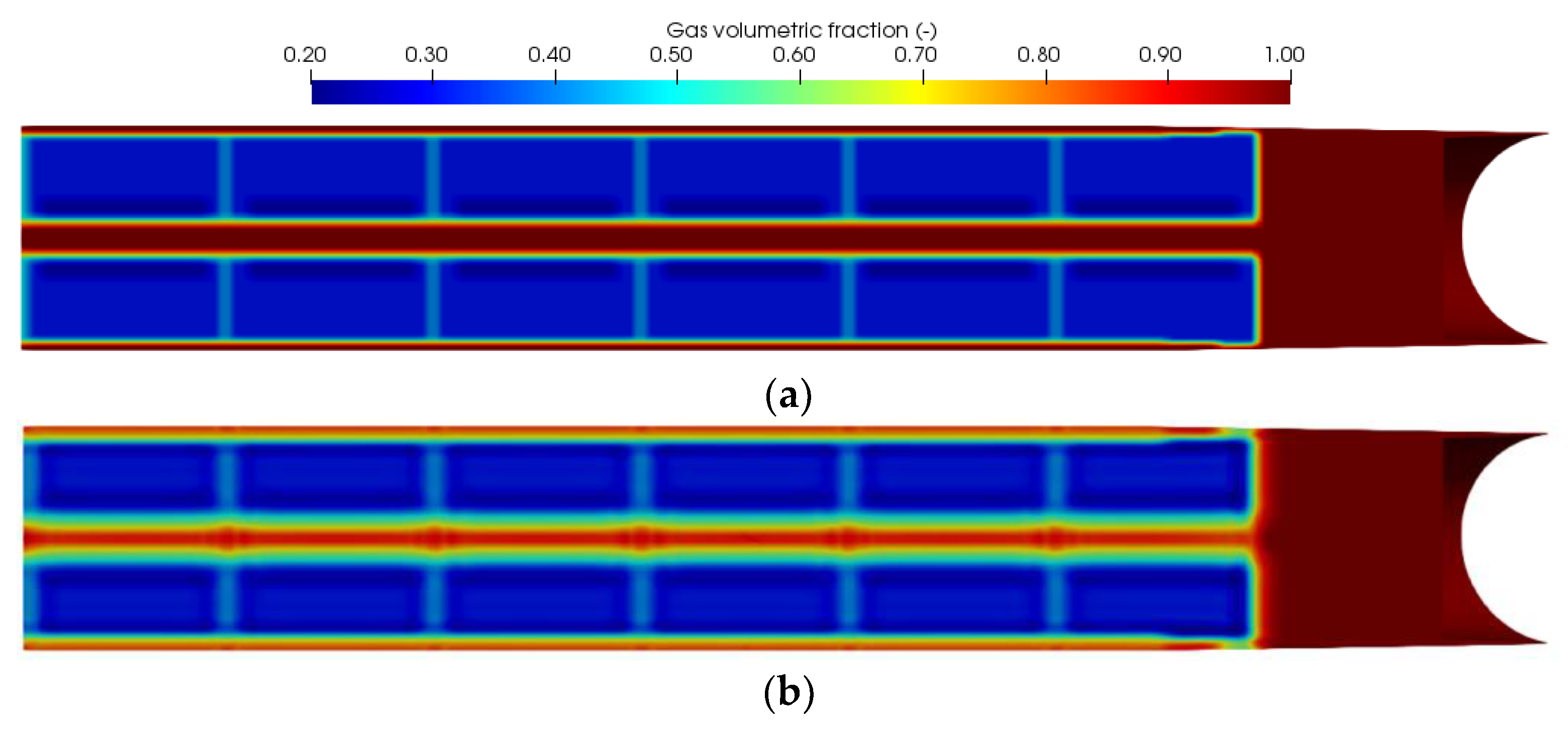
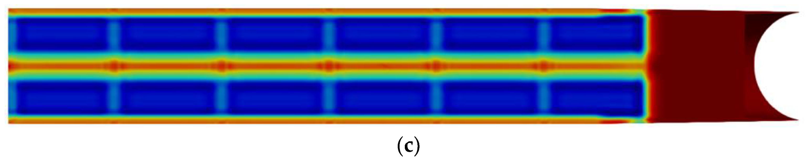
All in all, we can conclude from the results (Figure 9, Figure 10, Figure 11 and Figure 12) that by eliminating the intergranular stress term, for this specific case of MACS simulation, there is an improvement in the modeling of the initial moments of the combustion sequence, and the numerical result is less diffusive. To illustrate this, the firing of a six-module MACS in a 155/52 howitzer (chamber volume of 23 L) is simulated. The simplified geometry of Figure 6a is considered for the modules, whose interior is filled with 2.5 kg of extruded propellant in the shape of a 19-perforation rosette. For the case presented, a standard triple-base propellant composition M30 [26] was used, with a heat of explosion of 974 cal/g, specific heat ratio of 1.2385, covolume of 1.057 × 10⁻³ m³/kg, and density of 1660 kg/m³. For the burning rate, modeled after Equation (26), we consider the coefficients $a$ = 4.597 × 10⁻⁷ m/(s·Paⁿ), $n$ = 0.652, and $b$ = 0 [26]. The results of this simulation are represented in Figure 9, where, employing contour plots of the gas volume fraction ${\alpha }_1$, the evolution of solid concentration as the combustion process progresses is observed (considering that ${\alpha }_2=1-{\alpha }_1$). In this figure (and also in Video S2 of Supplementary Materials, where the results are represented with a higher temporal resolution for ${\alpha }_1$, pressure, temperature, and velocity), it is observed that, when the solid begins to burn through the area corresponding to the combustible case, ${\alpha }_1$ increases as the combustion source terms convert the solid phase into gas. 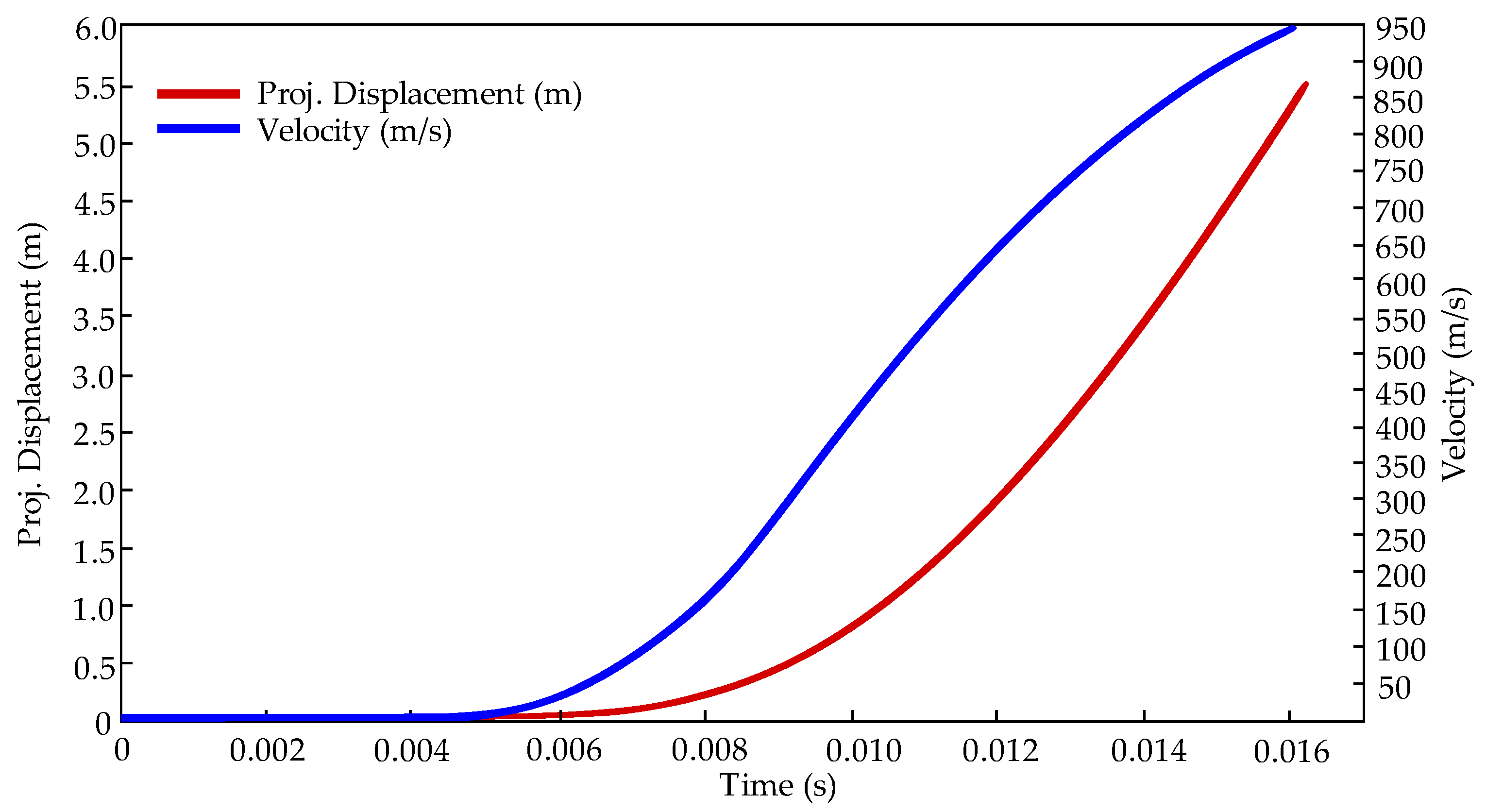In this process, temperature and pressure increase accordingly (see Video S2). The combustion process takes place on a time scale appropriate to the Internal Ballistics of a shot of the same characteristics. In fact, projectile motion starts at $t\approx 6$ ms (Figure 11) and is apparent to the naked eye (Figure 9 and Supplementary Video S2) at $t\approx 7$ ms. The entire ballistic cycle, from the ignition to the exit of the projectile through the muzzle, lasts 16.25 s (in howitzers of this type, the shot can be between 15 and 20 ms [25]). The outcomes of 2D Axisymmetric and 3D simulations (Figure 10) are practically identical, because the modules fill the whole diameter of the chamber and, therefore, in the 3D case, there is an almost concentric symmetry, like in the 2D Axisymmetric case.

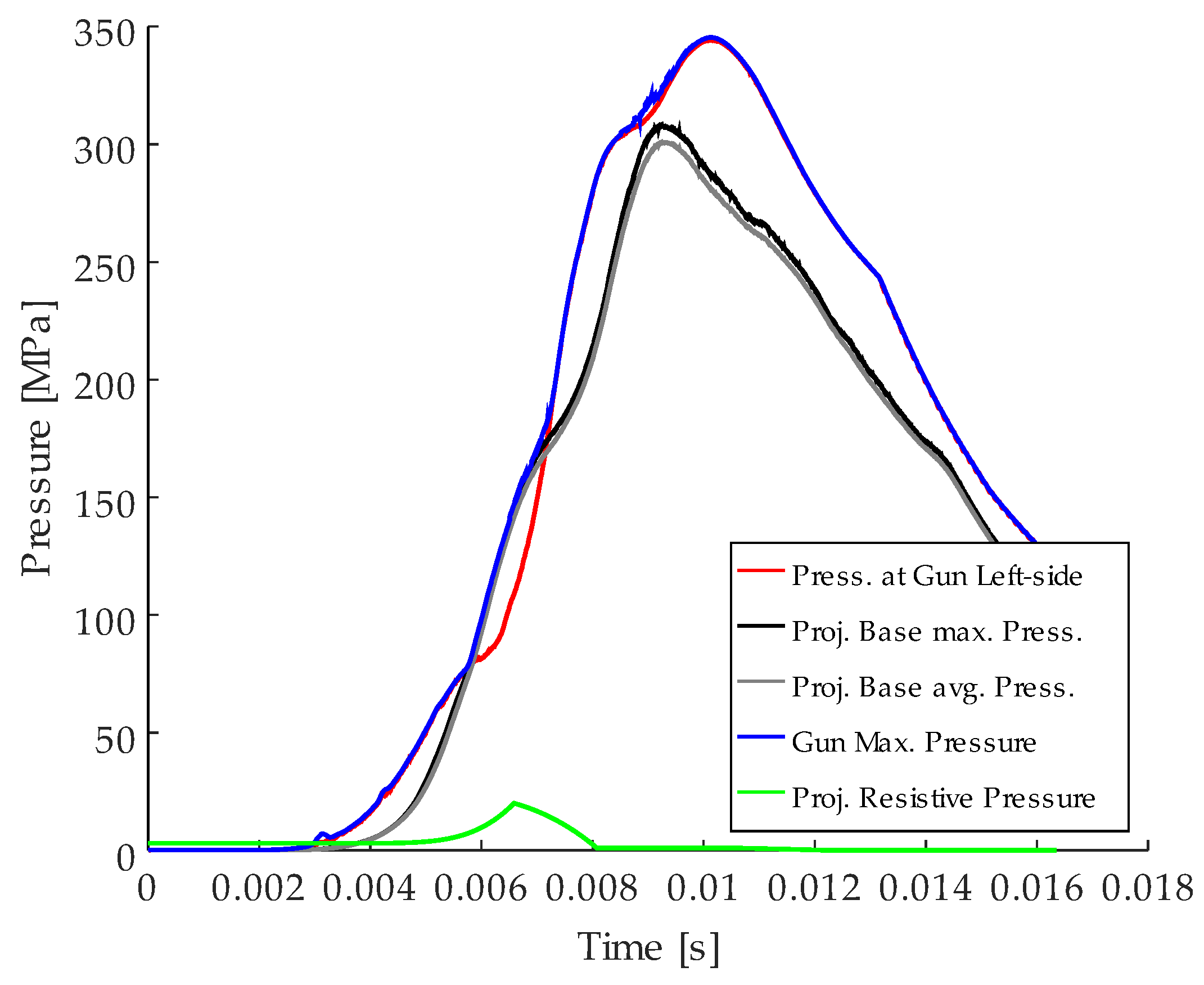
The results for muzzle velocity and chamber pressure obtained with the last simulation are those represented in Figure 11 and Figure 12. The pressure-time curve in Figure 12, with a maximum pressure of 349.25 MPa, corresponds to the expected curve in a modular charge shot, if the propellant used were an M30 composition (more energetic and faster than usual compositions of MACS) and the muzzle velocity, 940 m/s (i.e., the velocity of the projectile at the bore), corresponds to the nominal velocity of the system.

4. Conclusions

Relying on an Interior Ballistics model for numerical simulation is always a great help in the process of designing and characterizing propelling charges. If this mathematical and numerical model can predict three-dimensional effects in the combustion process, this would be an advantage, and even more so for the design of modular charges where geometric effects are of utmost importance. To do this, the mathematical models underlying the simulation tool must be reliable, validated, and provide accurate results.

With this objective, a model of conservation equations that are capable of describing the transient 3D combustion behavior of propellants inside the chamber of an artillery gun was presented in this work. Both the governing equations and the closure laws were described. In addition, the numerical methods used in their resolution were presented. This mathematical model was implemented in the new software UXGun3D, which was first tested by simulating the firing of a conventional projection charge, obtaining very satisfactory results. The study shows it is feasible to simulate with a Eulerian-Eulerian model of conservation equations the problem of modular charge firing. The results obtained are in line with the expected nominal values. The main challenges are the presence of various energetic materials (propellant, initiator, combustible case) and, mainly, the different mechanical and chemical behavior of the combustible cartridge cases. The propellant responds well to this type of model; however, for the combustible cases, diffusion is observed that is not physical for this type of material and that comes from the generation of momentum from the intergranular stress term. To overcome this drawback, simulations were carried out, avoiding the intergranular stress term and obtaining satisfactory results. As for the numerical methods, the approach proposed, based on a formulation of the system of equations in terms of conserved variables, and the numerical flux schemes proved to be a good choice for the solution of this complex problem. However, a non-physical numerical diffusion was observed where the eigenvalues were coupled in the numerical flux schemes. It was found that decoupled eigenvalues are preferable, so that the eigenvalues of each phase subsystem of equations are used for their own numerical flux schemes. This way, the final results are fully satisfactory and provide the expected pressure and muzzle velocity values.

Future work will focus on implementing an even more detailed model, in which a dedicated momentum equation is available for each species of the solid phase, so that the intergranular stress term can be enabled for gunpowder, while being deactivated for the solid case. Likewise, the work may be continued by carrying out more experimental tests.