1. Introduction
First proposed by Corrado Gini in 1912 [
1], the Gini coefficient or Gini index has been widely used in describing inequalities in various fields, such as income/wealth [
2], meteorology [
3], ecology [
4], hydrology [
5], water resources [
6], and the environment [
7]. However, accurate estimation of the Gini coefficient has been a continuing topic of investigation, especially for grouped data [
2,
8,
9,
10].
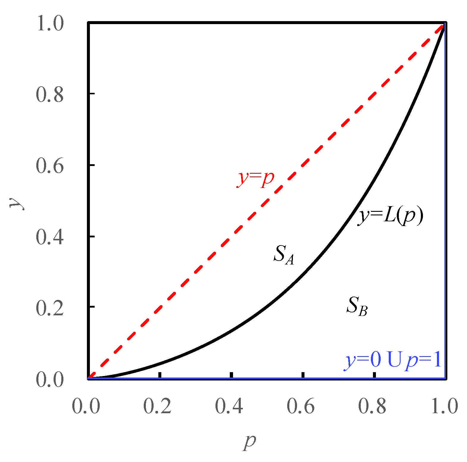
The Gini coefficient is an important index that is related with the Lorenz curve (
Figure 1), which was developed by Lorenz in 1905 [
11] and shows the cumulative share of income or another variable under consideration (
y [0, 1]) from different sections of population or another variable (
p [0, 1]). The Lorenz curve is a non-negative, monotonic increasing, and convex curve [
12,
13]. In
Figure 1, the straight diagonal line
y =
p represents perfect equality in income or other distribution, while a Lorenz curve
y =
L (
p) generally lies beneath the line of perfect equality. The area between the line
y =
p and curve
y =
L (
p),
SA, represents the inequality in income or other distribution. The greater the
SA, the greater the inequality in the distribution. Line segments
y = 0 and
p = 1 (
p,
y [0, 1]) with the greatest
SA = 1/2 represent another extreme distribution, the line of absolute inequality. The Gini coefficient, a scalar measurement of inequality, is defined as 2
SA for a Lorenz curve
y =
L (
p), which varies from 0 (representing perfect equality) to 1 (representing absolute inequality).
Besides estimation methods of the Gini coefficient directly from statistical data or its probability distribution, many estimation methods are based on the approximation of the corresponding Lorenz curve using curve fitting or interpolation methods, especially for grouped data.
The curving fitting method fits the data with functions that meet the requirements of the Lorenz curve, i.e., non-negativity, monotonicity, and convexity [
12,
13]. However, an appropriate function is usually selected from a group of possible functions for specified data, and the selected function is generally not flexible enough to depict the complex variation of actual data globally [
13]. Moreover, the fitted Lorenz curves can only represent the global trend and generally do not pass through all the data points, which is a common characteristic of the curve fitting method.
Contrary to the curve fitting method, the interpolation method constructs an interpolation curve that passes all data points. For grouped data, the simplest method to estimate the Gini coefficient is the trapezoidal rule, which approximates the Lorenz curve with piecewise linear interpolation. However, the trapezoidal rule always underestimates the Gini coefficient, and is generally taken as the lower limit of the Gini coefficient [
14]. To improve the estimation accuracy of the Gini coefficient, higher order numerical integration methods that approximate the Lorenz curve with piecewise polynomial interpolation, such as Simpson’s and Romberg’s rules, can be used [
14]. However, these numerical integration methods are generally applicable to equally spaced data except the trapezoidal rule. Furthermore, widely used Lagrangian, Hermite, and other interpolation curves do not necessarily preserve the non-negativity, monotonicity and convexity of the Lorenz curve [
8]. Therefore, monotonicity and convexity should be considered in interpolating the Lorenz curve.
Another problem in interpolating the Lorenz curve with Hermite or other similar interpolators is the estimating of derivatives at intermediate points and endpoints [
9], which has significant influence on the estimated Gini coefficient and should be considered with care in the interpolation.
The main objective of the present study is to develop a shape-preserving cubic Hermite interpolation method to approximate the Lorenz curve for estimating the Gini coefficient directly from the interpolation coefficients, where the derivatives of the Lorenz curve at intermediate points and endpoints are optimized by maximizing or minimizing the strain energy or curvature variation energy of the interpolation curve subject to non-negativity, monotonicity and convexity conditions. The applicability of this method was tested with 16 grouped datasets.
2. Materials and Methods
2.1. Conditions of Shape-Preserving Cubic Hermite Interpolation for the Lorenz Curve
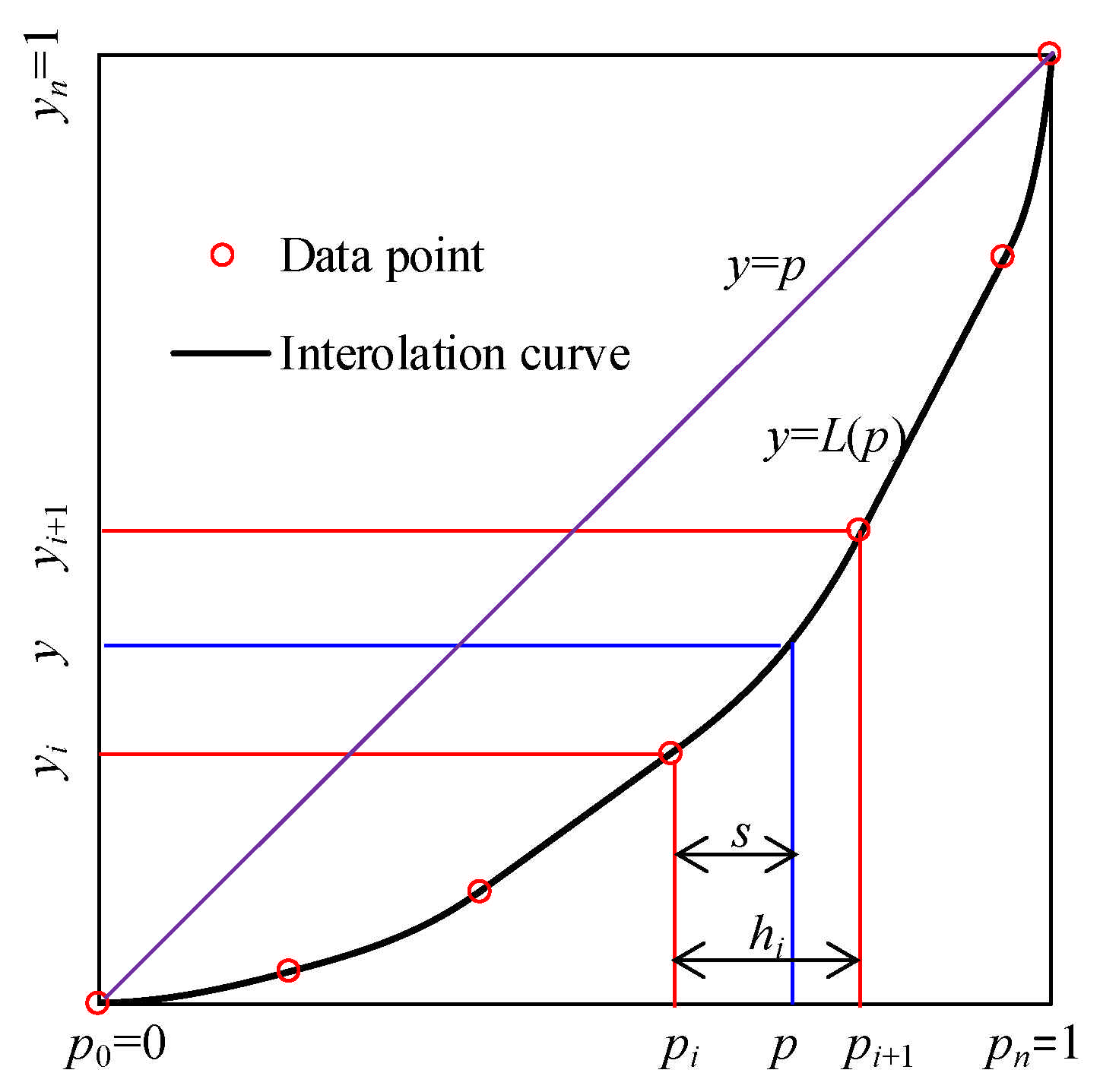
Suppose we have
n + 1 points in the Lorenz curve, (
pi,
yi),
i = 0, 1, …,
n, where 0 =
p0 <
p1 <…<
pn = 1 is the cumulative fractions of the population or other variable of interest, and 0 =
y0 <
y1 <…<
yn = 1 is the cumulative fractions of income or another variable (
Figure 2). The length of interval
Ii = [
pi,
pi+1],
hi, and slope of the line passing through (
pi,
yi) and (
pi+1,
yi+1),
δi, are denoted as:
Since the Lorenz curve is generally a convex curve, data points (
pi,
yi),
i = 0, 1, …,
n, form a strictly convex set, i.e.,
A continuously differentiable function,
L (
p), to approximate the Lorenz curve should pass all the interpolation points (
pi,
yi),
i = 0, 1, …,
n, and has the same derivative as the Lorenz curve at each interpolation point (
Figure 2). These conditions can be expressed as:
where
di is the derivative of the Lorenz curve at
pi,
i = 0, 1, …,
n. Generally,
di,
i = 0, 1, …,
n, are not known from statistics, and their estimation is essential for the interpolation and will be discussed later. The interpolation curve should have the same properties as the Lorenz curve, including non-negativity, monotonicity, and convexity.
A piecewise cubic Hermite interpolation curve that satisfies conditions (3) and (4) is [
15,
16]:
The first and second derivatives of the interpolation curve
L (
p) are
Following [
17], the necessary and sufficient condition for the convexity of the interpolated Lorenz curve can be determined. The convexity of the Lorenz curve requires that
,
i = 0, 1, …,
n − 1, which is equivalent to
and
,
i = 0, 1, …,
n − 1, because
is a linear function of
s. From Equation (8), the convexity of the interpolation curve can be preserved if and only if
or
If the convexity condition (9) is satisfied,
is a strictly monotonic increasing function. Therefore, the monotonic condition of
L (
p),
, is equivalent to
In this case, the monotonicity of L (p) is satisfied. Meanwhile, the non-negativity of L (p) is also valid because L (0) = 0.
In summary, if the convexity condition (9) and monotonicity condition (10) are satisfied, L (p) have the properties of non-negativity, monotonicity, and convexity, and can be used as an approximation of the Lorenz curve.
2.2. Construction of the Shape-Preserving Cubic Hermite Interpolation for the Lorenz Curve
Cubic spline,
S (
p), is the most widely used cubic Hermite interpolants, which has continuous derivatives to order two and minimizes some energy functions, such as the widely used strain energy [
18] and curvature variation energy [
19]. These two energy functions can be approximated as [
20]
where
Es and
Ec are approximated forms of strain energy and curvature variation energy, respectively.
However, S (p) constructed from the energy minimization does not necessarily preserve the properties of non-negativity, monotonicity or convexity. To construct a shape-preserving cubic Hermite interpolation for the Lorenz curve, we determined the derivatives di, i = 0, 1, …, n, by minimizing the energy function (11) or (12) subject to conditions (9) and (10).
For
L (
p), the approximated strain energy is
Because
is a constant in the interval
Ii = [
pi,
pi+1],
i = 0, 1, …,
n − 1, the approximated strain energy can be deduced to be
Meanwhile, the approximated curvature variation energy is
Therefore, the derivatives
di,
i = 0, 1, …,
n, can be determined from the following quadratic programming model:
or
subject to linear constraints (8) and (9). Compared with Equations (14) and (15), constants and items that have no influence on the optimal solution of the quadratic programming model are omitted in Equations (16) and (17).
Generally, the minimization of energy functions results in a straight and smooth spline. However, the straightness and smoothness are not intrinsic properties of a Lorenz curve. Following [
21], we also used an alternative criterion to define the constrained Lorenz curve, i.e., maximizing the strain energy or curvature variation energy functions using Equation (18) or (19) subject to linear constraints (9) and (10).
In contrast to the straight and smooth spline resulted from (16) or (17), spline resulted from (18) or (19) will contain relatively sharp curvatures or curvature variations. These two types of splines represent the most and least smooth interpolation curves that meet the requirements of the Lorenz curve, and will be compared to find which is more appropriate to approximate the Lorenz curve.
Now we have four optimization models with the objective functions of (16)–(19) subject to constraints (9) and (10). Due to diversity in empirical points (
pi,
yi),
i = 0, 1, …,
n, and the estimated
δi,
i = 0, 1, …,
n − 1, it is difficult to obtain the optimal solution analytically using the Kuhn-Tucker condition for nonlinear programming [
22]. Because the feasibility region bounded by the linear constraints (9) and (10) are a convex set and the second order items in objective function (16) and (17) are positive definite and positive semi-definite, respectively, the minimizations of strain energy and curvature variation energy are both convex programming that have a unique optimal solution.
Moreover, from inequalities (2), (9), and (10), we have
Therefore, all decision variables (di, i = 0, 1, …, n), and corresponding objective functions (18) and (19) are finite with lower and upper limits. Consequently, objective functions (18) and (19) have maximum in the feasibility region.
To solve the above quadratic programming models, several algorithms and optimization tools can be used [
22], among which the Microsoft Excel Solver was chosen because of its wide availability and easy applicability [
23].
2.3. Estimating Gini Coefficient from the Interpolated Lorenz Curve
The Gini coefficient,
G, can be estimated directly from the coefficients of the interpolated Lorenz curve (
Figure 2) using the following formula.
Using trapezoidal rule that approximates the Lorenz curve with piecewise linear interpolation, the estimated Gini coefficient,
GT, is usually taken as its lower bound, which is
From Equations (21) and (22),
G can be estimated from
Because of the convexity of the interpolated Lorenz curve, its first derivative, d (p), is a monotonic increasing function. Therefore, G estimated with Equation (23) is always greater than its lower bound of GT. Meanwhile, for a grouped dataset with known yi, i = 0, 1, …, n, and hi, i = 0, 1, …, n − 1, G depends only on the estimated derivatives of the interpolated Lorenz curve, especially the right part of the curve that has significantly greater derivative. Because the derivative at the left endpoint is small and the influence of derivatives at intermediate points can be partly (for unequally spaced data) or completely (for equally spaced data) counterbalanced for successive intervals from Equation (23), accurate estimation of derivatives at intermediate points and endpoints is crucial for accurate estimation of G, especially the derivative at the right endpoint.
When the grouped data is equally spaced with equal interval lengths of
h, Equation (23) can be further simplified to
This equation further illustrates the importance of accurately estimating the derivatives at the endpoints, especially the right endpoint.
2.4. Data Used to Test the Method
To test the applicability of the interpolated Lorenz curve in estimating the Gini coefficient and to find whether minimizing or maximizing the strain energy or curvature variation energy is more preferable, we used 16 grouped datasets from published references to estimate their Gini coefficients, and compared the results with the “true” values estimated from all census data and estimates using other methods. These datasets include quintiles [
24,
25], quintiles plus the 95th percentile [
10], and an unequally spaced dataset [
26].
3. Results
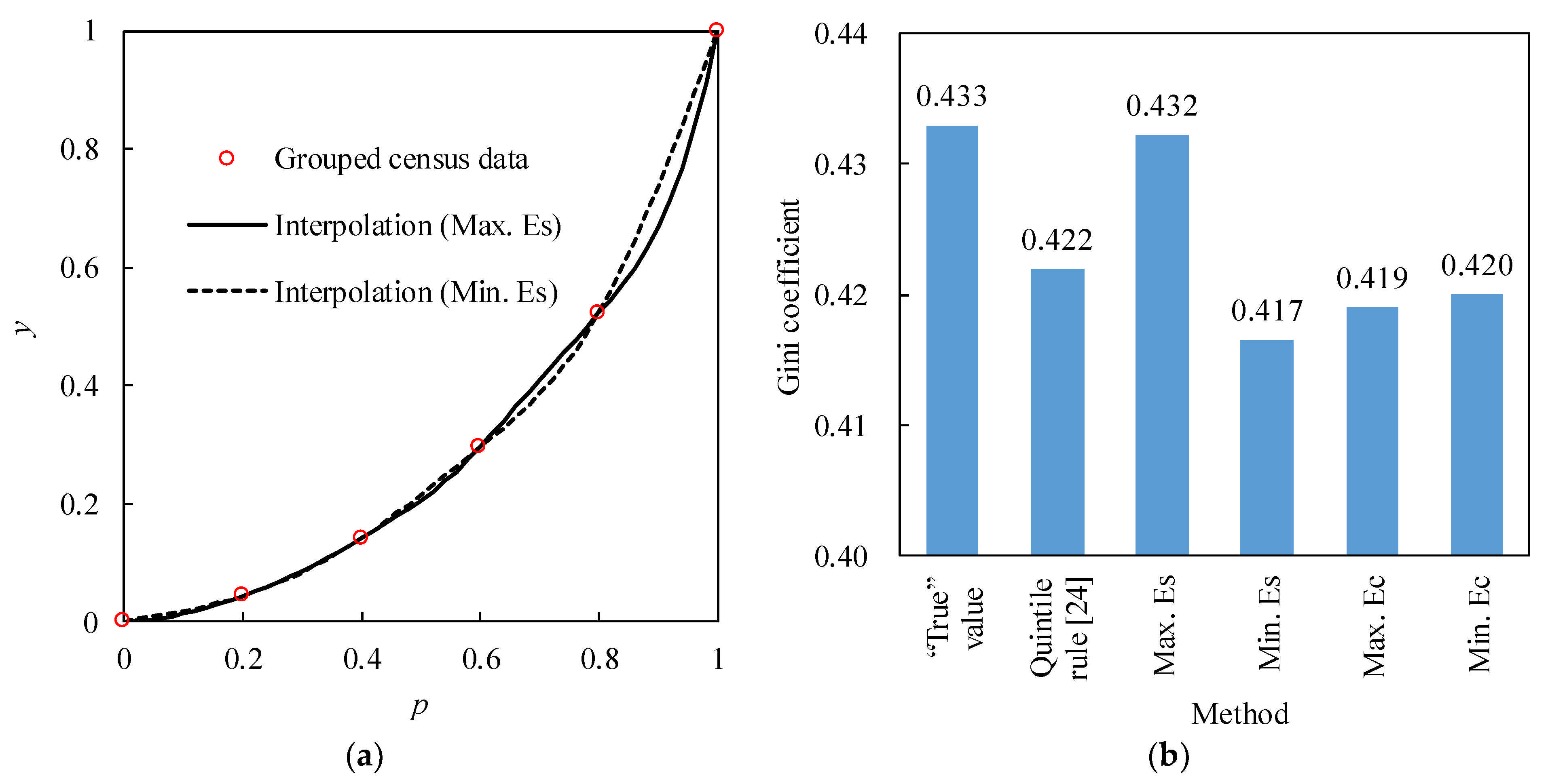
The interpolated Lorenz curves for the grouped quintiles of US income census data in 2000 [
24] by minimizing or maximizing the approximated strain energy are shown in
Figure 3a, which shows that the former (Min. Es) is smoother than the latter (Max. Es). Meanwhile, negative and positive differences between these two interpolation curves occur alternatively in adjacent intervals, and the maximum absolute value of the differences in these intervals tend to increase with the cumulative population fraction (
p). The maximum difference of 0.075 occurs at
p = 0.92 in the last interval [0.8, 1]. Gini coefficients (
G) estimated with these two interpolated Lorenz curves are 0.417 and 0.432, respectively; while
G estimated with the interpolated Lorenz curves (not shown in
Figure 3a for clarity) by minimizing (Min. Ec) and maximizing (Max. Ec) the approximated curvature variation energy are 0.420 and 0.419, respectively. Compared with the estimates using the quintile rule of 0.422 [
24], the estimated
G corresponding to Max. Es interpolation of 0.432 is very close to the “true” value of 0.433 calculated from all the census data (
Figure 3b), and is superior to other methods.
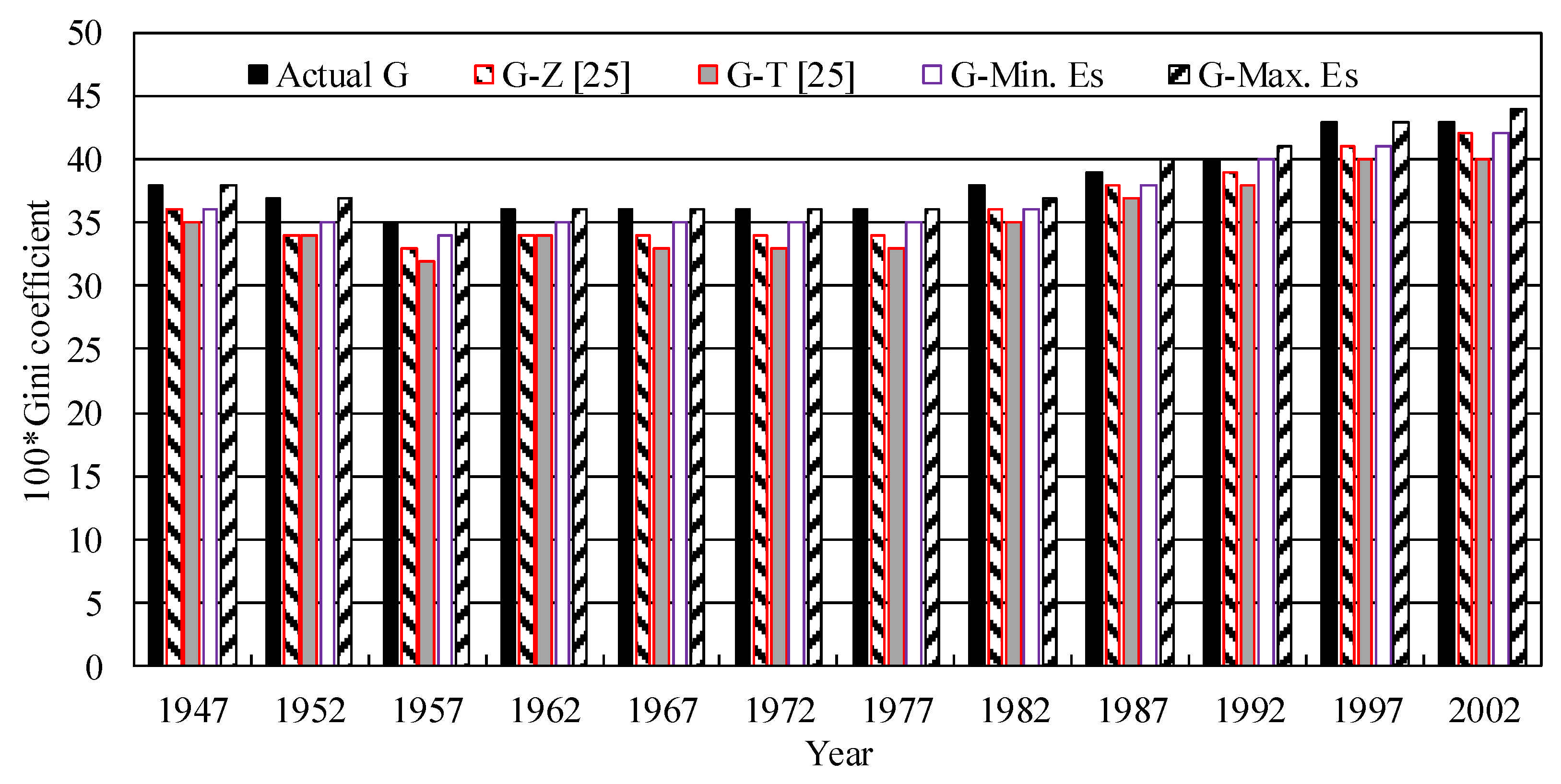
Using income quintiles of the United States in five-year intervals from 1947 to 2002 [
20], the Gini coefficients were estimated with the present interpolation method and compared with those with Z-gradient and trapezoid rules [
25] (
Figure 4). For comparison purposes, all the
G values were rounded to two decimals (or integers for 100G) as in [
25]. From
Figure 4, absolute errors between the actual values of 100G calculated from all census data and 100G estimated with the Z-gradient rule, trapezoid rule, Min. Es interpolation, and Max. Es interpolation range from 1–3, 2–3, 0–2, and 0–1 with the average values of 1.8, 2.8, 1.3, and 0.3, respectively. The average absolute error of
G estimated with the Max. Es interpolation is only 12% to 27% of those with the other three methods.
G is generally underestimated by the Z-gradient and trapezoid rules and the Min. Es interpolation method, while
G estimates using the Max. Es interpolation method is the closest to the actual value.
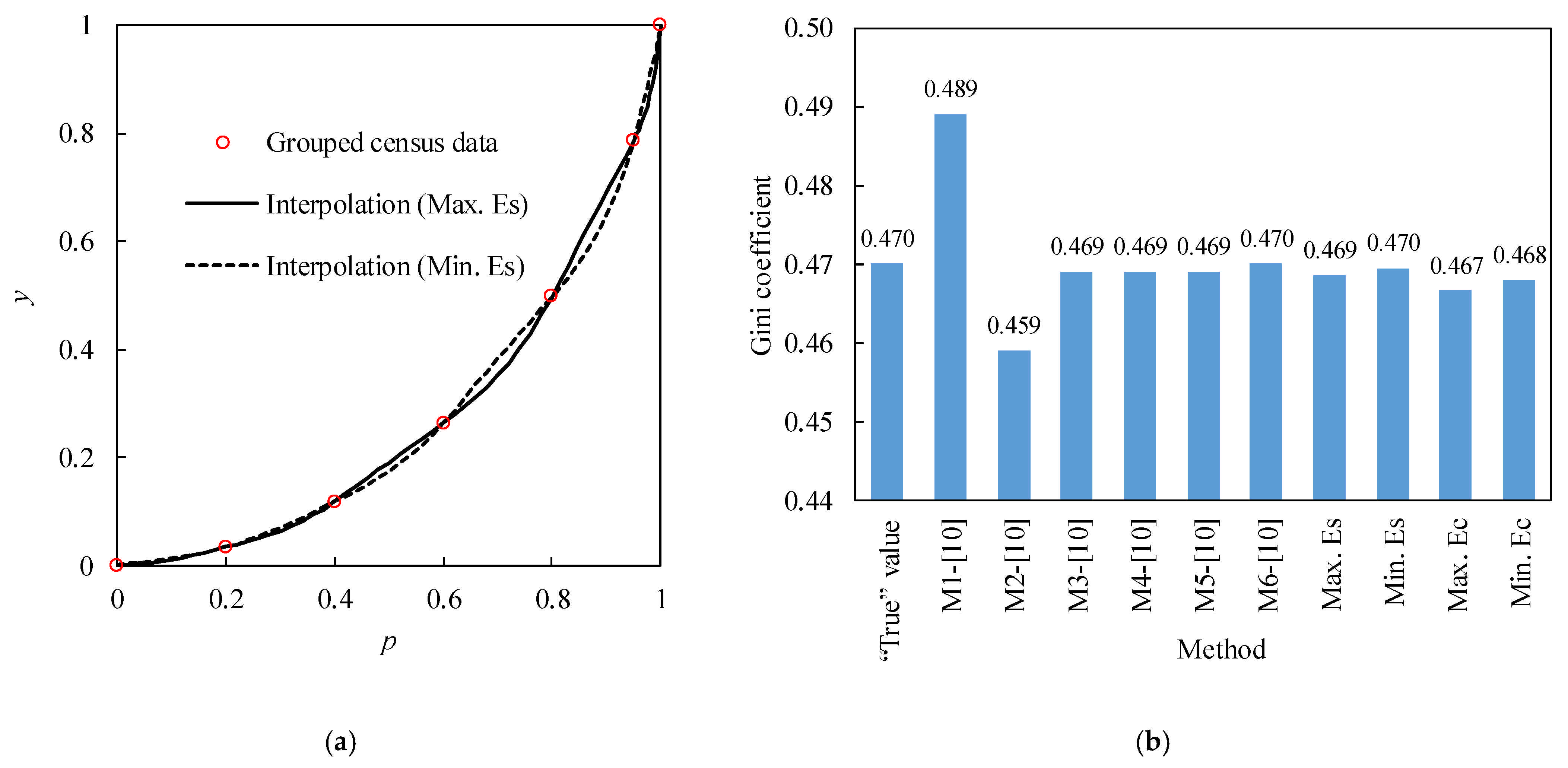
The interpolated Lorenz curves for the grouped quintiles plus the 95th percentile of US income census data in 2010 [
10] are shown in
Figure 5a. Similar to
Figure 3a,
Figure 5a also shows that the interpolated curve by Min. Es interpolation is smoother than that by Max. Es interpolation, and their maximum differences in successive intervals tend to increase with
pi for
pi < 0.95, which reach the peak of 0.043 when
pi = 0.89. However, the difference becomes smaller for
pi > 0.95 due to the added data at
pi = 0.95 and the shorter interval.
G estimated with these two interpolated Lorenz curves are 0.470 and 0.469, respectively, which are the same or very close to the “true” value of 0.470.
G estimated with Max. Ec and Min Ec also give satisfactory results of 0.467 and 0.468, respectively, which are slightly poorer than
G estimated with Max. Es and Min Es. Among six methods used in [
10], four methods also gave very good
G estimates of 0.467 to 0.470, while two other methods resulted in poorer estimates compared to the aforementioned results (
Figure 5b).
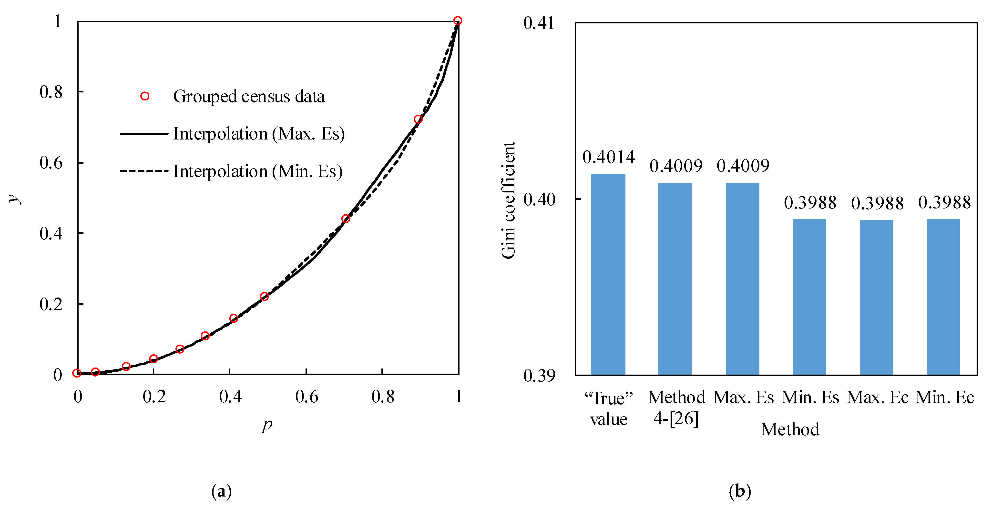
The interpolated Lorenz curves for the income data of 10 unequally spaced groups [
26] are shown in
Figure 6a. For
pi < 0.492 that has interval lengths less than 0.08, the differences between two interpolated Lorenz curve with Max. Es and Min. Es are very small. However, the difference becomes greater with the longer interval when
pi > 0.492, and reaches its peak of 0.042 at
pi = 0.959. Gini coefficients (
G) estimated with these two interpolated Lorenz curves are 0.3988 and 0.4009 (
Figure 6b), respectively.
G is slightly underestimated using the Min. Es interpolation method. Meanwhile, the estimated
G based on Max. Es is the same as the estimates using the method 4 in [
26], which are both very close to the “true” value of 0.4014 calculated from all the census data. Values of
G estimated with Max. Ec and Min. Ec are close to that estimated with Min Es., but they are all slightly poorer than
G estimated with Max. Es.
4. Discussion and Conclusions
The Gini coefficient is widely used in describing inequalities in many fields, but its accurate estimation is still difficult for grouped data with fewer groups. We proposed a shape-preserving cubic Hermite interpolation method to approximate the Lorenz curve by maximizing or minimizing the approximated strain energy or curvature variation energy of the interpolated curve, which can then be used to estimate the Gini coefficient directly from the interpolation coefficients. Case studies with 16 grouped quintiles or unequally spaced datasets (
Figure 3,
Figure 4,
Figure 5 and
Figure 6) showed that the maximum strain energy interpolation method generally performs the best among different methods compared with the “true” Gini coefficient calculated with all census data.
The proposed shape-preserving cubic Hermite interpolation method for the Lorenz curve has several advantages. First, the interpolated curves pass all data points, which is preferable to fitted curves that are generally not flexible enough to depict the complex variation of actual data globally and do not pass all data points [
13]. Second, the interpolated curve preserves the essential requirements of the Lorenz curve, i.e., non-negativity, monotonicity, and convexity [
17]. Third, derivatives at intermediate points and endpoints are optimized at the same time by maximizing or minimizing the energy functions subject to non-negativity, monotonicity, and convexity conditions (9) and (10), which is much simpler than some other interpolation methods that determine derivatives at intermediate points and endpoints with different methods [
9]. Because accurate estimation of derivatives at intermediate points and endpoints, especially the derivative at the right endpoint, is crucial for accurate estimation of
G, the simultaneous estimation of derivatives at intermediate points and endpoints may be a possible reason for the higher precision of the estimated
G. Fourth, the method is applicable to both equally and unequally spaced grouped datasets with higher precision than other methods, especially for datasets with fewer groups (
Figure 3,
Figure 4 and
Figure 5). The estimated Gini coefficients using the maximizing strain energy rule are better than or close to other methods for most of the case studies.
The Lorenz curve generated from the minimizing strain/curvature variation energies are smoother than those from the maximizing strain/curvature variation energies. These two types of interpolated Lorenz curves represent the most and least smooth interpolation curves that meet the requirements of the Lorenz curve, and their differences tend to increase with the population fraction and interval length (
Figure 3,
Figure 5 and
Figure 6). The Lorenz curve interpolated from the maximizing strain energy generally contains relatively sharp curvatures that may better reflect the distribution of income or other variables under consideration within each group, and results in better estimation of derivatives at intermediate points and endpoints, which is the possible reason for better estimates for the Gini coefficient using the maximizing strain energy rule compared with other energy rules.


