
Machine Learning Applied to the Oxygen-18 Isotopic Composition, Salinity and Temperature/Potential Temperature in the Mediterranean Sea


Abstract
:1. Introduction
- Artificial neural networks are a computational method inspired on the cell of the nervous system (known as neuron) [19] to try to analyse and reproduce the learning mechanism that owned by the more highly evolved animal species [20]. These models can find the relationships between inputs and outputs variables [21]. When the relationships are complex and highly non-linear, this kind of model needs a relatively huge training data group [22]. The ANNs are used as an option to statistical methods for different purposes such as estimation, classification, among others [23]. ANN approaches are popular due to their flexibility to fit random data and their reasonably uncomplicated development [23,24]. As previously stated, ANN models developed in this research are based on an MLP neural network, a popular ANN architecture [25]. ANNs are applied in different fields such as chemistry [26], medicine [27], food authenticity [28], among others [29,30]. This type of model can be part of more complex systems such as a smart healthcare monitoring system to predict heart disease that used ensemble deep learning [31] or to classify skin disease through deep learning neural networks stand on MobileNet V2 and long short-term memory [32].
- The second kind of model used is a random forest model. RF is a computational method for regression and/or classification [36] proposed by Breiman (2001) [36,37]. A random forest model is formed by decision trees where each tree utilizes a sample subset of available data [38], and the random forest’s prediction value is the average of all predicted values [38,39]. Random forest is one of the most capable machine learning approaches for forecasting [40] and can be used in different fields such as environmental science [38] and chemistry [41], among others [42,43].
- Finally, the last model developed is a support vector machine. An SVM model is a method enunciated by Boser et al. in 1992 [47,48]. Originally, the SVM models were developed for pattern recognition, nevertheless, nowadays they can be used to solve nonlinear regression problems or time series prediction [49,50] and due to its mathematical simplicity it has received much attention lately [51]. An SVM model creates a hyperplane, or hyperplanes, in a high- or infinite- dimensional space [52]. The hyperplane separates the dataset into a number of classes consistently with the training examples [53]. The principal advantage of SVM (compared to other classification techniques such as partial least square discriminant analysis) is its flexibility to model non-linear classification problems [54]. SVM models can be used in different areas such as: Engineering [55,56], Medicine [57,58], among others [59,60]. Related to this research field, SVM models can be used to estimate the SST in the tropical Atlantic [61] or to forecast the tropical Pacific SST anomalies [62]. In this case, Aguilar-Martinez used support vector regression and was compared with Bayesian neural network and linear regression models.
2. Materials and Methods
2.1. Database Used
2.2. Experimental Design
2.3. Methodologies
2.4. Fitting of Data and Modelling
2.5. Computational Resources
3. Results and Discussion
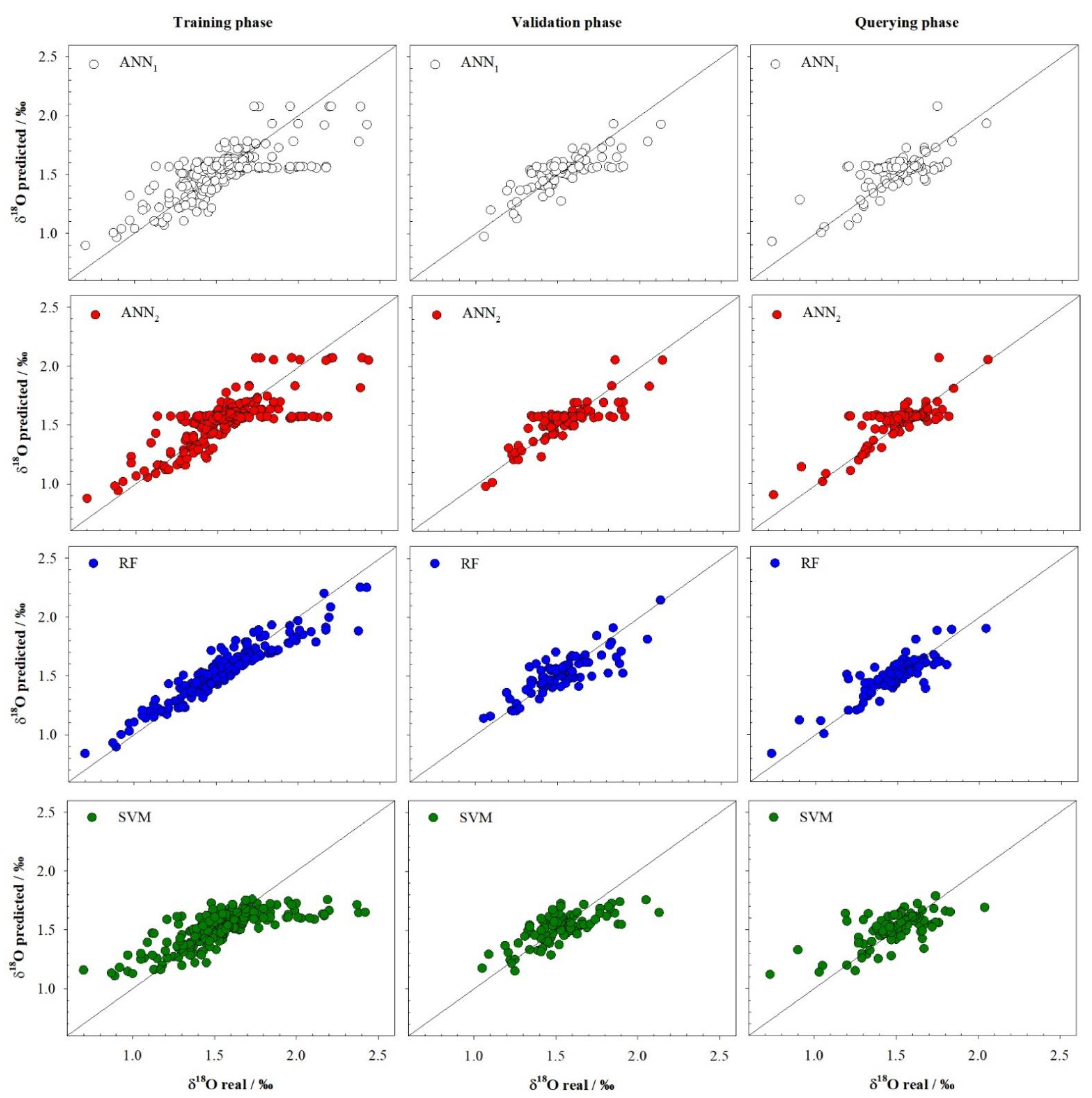
3.1. δ18 O Model
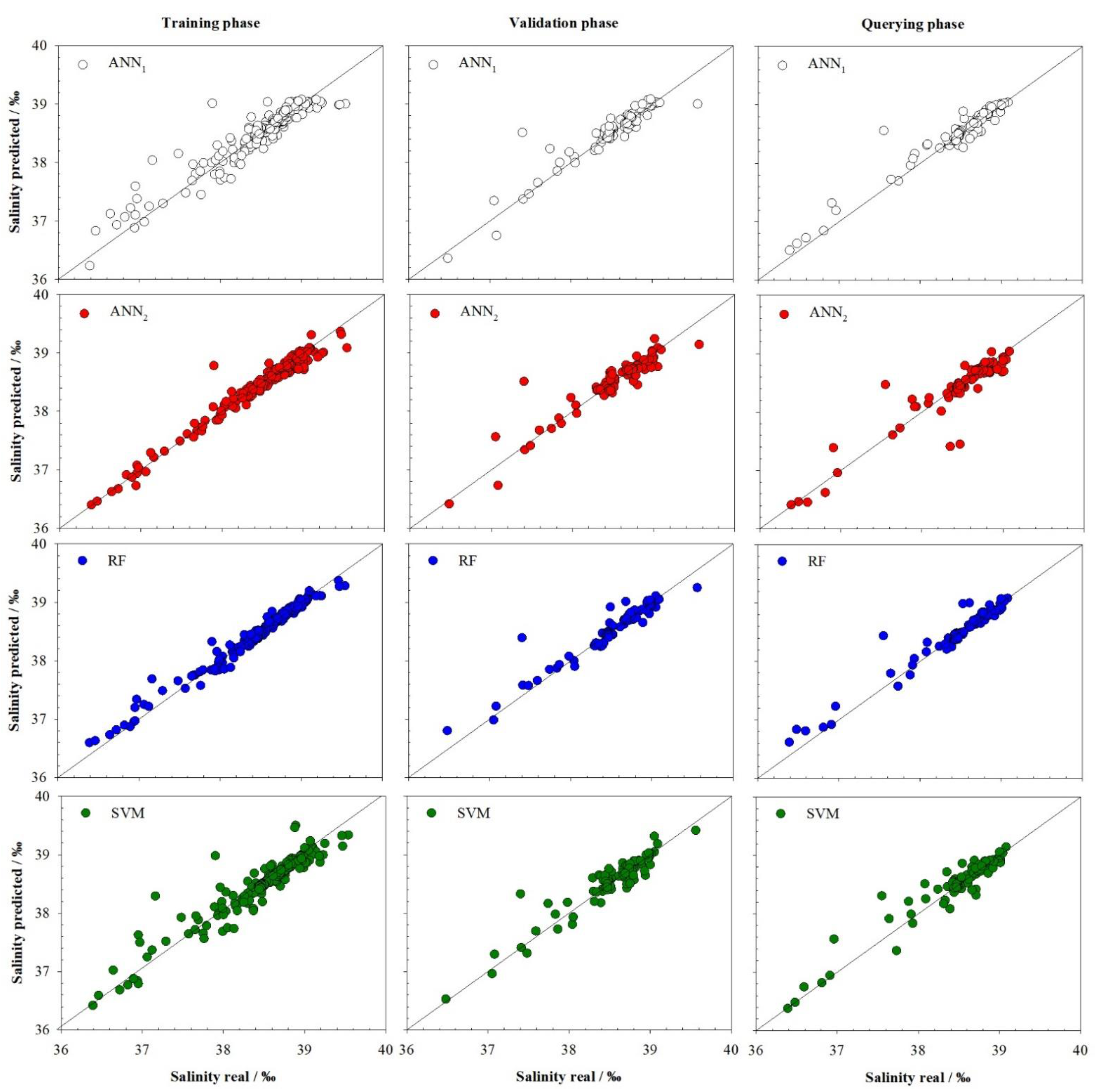
3.2. Salinity Model
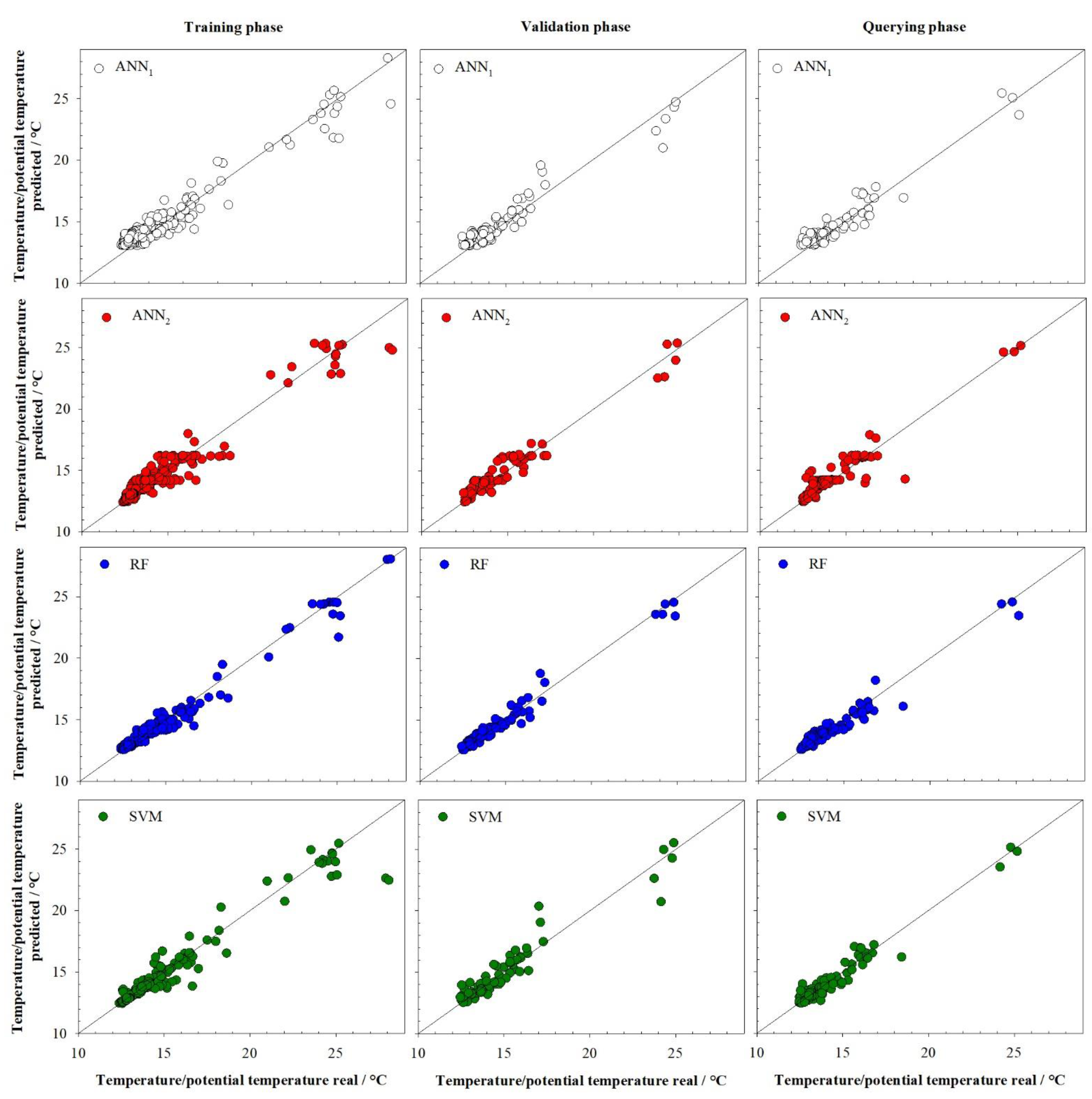
3.3. Temperature/Potential Temperature Model
4. Conclusions
Author Contributions
Funding
Institutional Review Board Statement
Informed Consent Statement
Data Availability Statement
Acknowledgments
Conflicts of Interest
References
- Theodor, M.; Schmiedl, G.; Mackensen, A. Stable Isotope Composition of Deep-Sea Benthic Foraminifera Under Contrasting Trophic Conditions in the Western Mediterranean Sea. Mar. Micropaleontol. 2016, 124, 16–28. [Google Scholar] [CrossRef]
- Gonzalez-Mora, B.; Sierro, F.J.; Schönfeld, J. Temperature and Stable Isotope Variations in Different Water Masses from the Alboran Sea (Western Mediterranean) between 250 and 150 Ka. Geochem. Geophys. Geosyst. 2008, 9, 1–14. [Google Scholar] [CrossRef] [Green Version]
- Rohling, E.J.; Marino, G.; Grant, K.M. Mediterranean Climate and Oceanography, and the Periodic Development of Anoxic Events (Sapropels). Earth Sci. Rev. 2015, 143, 62–97. [Google Scholar] [CrossRef]
- Herbert, T.D.; Ng, G.; Cleaveland Peterson, L. Evolution of Mediterranean Sea Surface Temperatures 3.5-1.5 Ma: Regional and Hemispheric Influences. Earth Plan. Sci. Lett. 2015, 409, 307–318. [Google Scholar] [CrossRef]
- Schroeder, K.; Garcìa-Lafuente, J.; Josey, S.A.; Artale, V.; Nardelli, B.B.; Carrillo, A.; Gacic, M.; Gasparini, G.P.; Herrmann, M.; Lionello, P.; et al. Circulation of the mediterranean sea and its variability. In The Climate of the Mediterranean Region; Lionello, P., Ed.; Elsevier: London, UK, 2012; pp. 187–256. [Google Scholar]
- Roberts, C.N.; Zanchetta, G.; Jones, M.D. Oxygen Isotopes as Tracers of Mediterranean Climate Variability: An Introduction. Glob. Planet. Chang. 2010, 71, 135–140. [Google Scholar] [CrossRef]
- Pierre, C. The Oxygen and Carbon Isotope Distribution in the Mediterranean Water Masses. Mar. Geol. 1999, 153, 41–55. [Google Scholar] [CrossRef]
- Tanhua, T.; Hainbucher, D.; Schroeder, K.; Cardin, V.; Álvarez, M.; Civitarese, G. The Mediterranean Sea System: A Review and an Introduction to the Special Issue. Ocean Sci. 2013, 9, 789–803. [Google Scholar] [CrossRef] [Green Version]
- Banaru, D.; Carlotti, F.; Barani, A.; Grégori, G.; Neffati, N.; Harmelin-Vivien, M. Seasonal Variation of Stable Isotope Ratios of Size-Fractionated Zooplankton in the Bay of Marseille (NW Mediterranean Sea). J. Plankton Res. 2014, 36, 145–156. [Google Scholar] [CrossRef] [Green Version]
- Estrada, M. Primary Production in the Northwestern Mediterranean. Sci. Mar. 1996, 60, 55–64. [Google Scholar]
- Stratford, K.; Williams, R.G. A Tracer Study of the Formation, Dispersal, and Renewal of Levantine Intermediate Water. J. Geophys. Res. Ocean. 1997, 102, 12539–12549. [Google Scholar] [CrossRef]
- Stratford, K.; Williams, R.G.; Drakopoulos, P.G. Estimating Climatological Age from a Model-Derived Oxygen–age Relationship in the Mediterranean. J. Mar. Syst. 1998, 18, 215–226. [Google Scholar] [CrossRef]
- Gat, J.R.; Shemesh, A.; Tziperman, E.; Hecht, A.; Georgopoulos, D.; Basturk, O. The Stable Isotope Composition of Waters of the Eastern Mediterranean Sea. J. Geophys. Res. C Ocean. 1996, 101, 6441–6451. [Google Scholar] [CrossRef]
- Fry, F.; Sherr, E. d13C Measurements as Indicators of Carbon Flow in Marine and Freshwater Ecosystems. Contrib. Mar. Sci. 1984, 27, 13–47. [Google Scholar]
- Bédard, P.; Hillaire-marcel, C.; Pagé, P. 18O Modelling of Freshwater Inputs in Baffin Bay and Canadian Arctic Coastal Waters. Nature 1981, 293, 287–289. [Google Scholar] [CrossRef]
- Sarkar, P.P.; Janardhan, P.; Roy, P. Prediction of Sea Surface Temperatures using Deep Learning Neural Networks. SN Appl. Sci. 2020, 2, 1458. [Google Scholar] [CrossRef]
- Zuo, X.; Zhou, X.; Guo, D.; Li, S.; Liu, S.; Xu, C. Ocean Temperature Prediction Based on Stereo Spatial and Temporal 4-D Convolution Model. IEEE Geosci. Remote Sens. Lett. 2021, 1–5. [Google Scholar] [CrossRef]
- Zhang, Z.; Pan, X.; Jiang, T.; Sui, B.; Liu, C.; Sun, W. Monthly and Quarterly Sea Surface Temperature Prediction Based on Gated Recurrent Unit Neural Network. J. Mar. Sci. Eng. 2020, 8, 249. [Google Scholar] [CrossRef] [Green Version]
- Gonzalez-Fernandez, I.; Iglesias-Otero, M.; Esteki, M.; Moldes, O.A.; Mejuto, J.C.; Simal-Gandara, J. A Critical Review on the use of Artificial Neural Networks in Olive Oil Production, Characterization and Authentication. Crit. Rev. Food Sci. Nutr. 2019, 59, 1913–1926. [Google Scholar]
- Sánchez-Mesa, J.A.; Galan, C.; Martínez-Heras, J.A.; Hervás-Martínez, C. The use of a Neural Network to Forecast Daily Grass Pollen Concentration in a Mediterranean Region: The Southern Part of the Iberian Peninsula. Clin. Exp. Allergy 2002, 32, 1606–1612. [Google Scholar] [CrossRef]
- Falah, F.; Rahmati, O.; Rostami, M.; Ahmadisharaf, E.; Daliakopoulos, I.N.; Pourghasemi, H.R. Artificial Neural Networks for Flood Susceptibility Mapping in Data-Scarce Urban Areas. In Spatial Modeling in GIS and R for Earth and Environmental Sciences; Hamid Reza Pourghasemi, C., Gokceoglu, A., Eds.; Elsevier: Amsterdam, The Netherlands, 2019; pp. 323–336. [Google Scholar]
- Hijazi, A.; Al-Dahidi, S.; Altarazi, S. A Novel Assisted Artificial Neural Network Modeling Approach for Improved Accuracy using Small Datasets: Application in Residual Strength Evaluation of Panels with Multiple Site Damage Cracks. Appl. Sci. 2020, 10, 8255. [Google Scholar] [CrossRef]
- Aparna, S.G.; D’Souza, S.; Arjun, N.B. Prediction of Daily Sea Surface Temperature using Artificial Neural Networks. Int. J. Remote Sens. 2018, 39, 4214–4231. [Google Scholar] [CrossRef]
- Patil, K.; Deo, M.C. Prediction of Daily Sea Surface Temperature using Efficient Neural Networks. Ocean Dyn. 2017, 67, 357–368. [Google Scholar] [CrossRef]
- Dawson, C.W.; Wilby, R.L. Hydrological Modelling using Artificial Neural Networks. Prog. Phys. Geogr. 2001, 25, 80–108. [Google Scholar] [CrossRef]
- Cid, A.; Astray, G.; Manso, J.A.; Mejuto, J.C.; Moldes, O.A. Artificial Intelligence for Electrical Percolation of Aot-Based Microemulsions Prediction. Tenside Surfactants Deterg. 2011, 48, 477–483. [Google Scholar] [CrossRef]
- Papadopoulos, A.; Fotiadis, D.I.; Likas, A. Characterization of Clustered Microcalcifications in Digitized Mammograms using Neural Networks and Support Vector Machines. Artif. Intell. Med. 2005, 34, 141–150. [Google Scholar] [CrossRef]
- Astray, G.; Mejuto, J.C.; Martínez-Martínez, V.; Nevares, I.; Alamo-Sanza, M.; Simal-Gandara, J. Prediction Models to Control Aging Time in Red Wine. Molecules 2019, 24, 826. [Google Scholar] [CrossRef] [Green Version]
- Makarynskyy, O. Improving Wave Predictions with Artificial Neural Networks. Ocean Eng. 2004, 31, 709–724. [Google Scholar] [CrossRef]
- Iglesias-Otero, M.A.; Fernández-González, M.; Rodríguez-Caride, D.; Astray, G.; Mejuto, J.C.; Rodríguez-Rajo, F.J. A Model to Forecast the Risk Periods of Plantago Pollen Allergy by using the ANN Methodology. Aerobiologia 2015, 31, 201–211. [Google Scholar] [CrossRef]
- Ali, F.; El-Sappagh, S.; Islam, S.M.R.; Kwak, D.; Ali, A.; Imran, M.; Kwak, K. A Smart Healthcare Monitoring System for Heart Disease Prediction Based on Ensemble Deep Learning and Feature Fusion. Inf. Fusion 2020, 63, 208–222. [Google Scholar] [CrossRef]
- Srinivasu, P.N.; SivaSai, J.G.; Ijaz, M.F.; Bhoi, A.K.; Kim, W.; Kang, J.J. Classification of Skin Disease using Deep Learning Neural Networks with MobileNet V2 and LSTM. Sensors 2021, 21, 2852. [Google Scholar] [CrossRef]
- Buongiorno Nardelli, B. A Deep Learning Network to Retrieve Ocean Hydrographic Profiles from Combined Satellite and in Situ Measurements. Remote Sens. 2020, 12, 3151. [Google Scholar] [CrossRef]
- Chen, W.; Liu, W.; Huang, W.; Liu, H. Prediction of Salinity Variations in a Tidal Estuary using Artificial Neural Network and Three-Dimensional Hydrodynamic Models. Comput. Water Energy Environ. Eng. 2017, 6, 107–128. [Google Scholar] [CrossRef] [Green Version]
- Cerar, S.; Mezga, K.; Žibret, G.; Urbanc, J.; Komac, M. Comparison of Prediction Methods for Oxygen-18 Isotope Composition in Shallow Groundwater. Sci. Total Environ. 2018, 631–632, 358–368. [Google Scholar] [CrossRef] [PubMed]
- Tian, Y.; Yan, C.; Zhang, T.; Tang, H.; Li, H.; Yu, J.; Bernard, J.; Chen, L.; Martin, S.; Delepine-Gilon, N.; et al. Classification of Wines According to their Production Regions with the Contained Trace Elements using Laser-Induced Breakdown Spectroscopy. Spectrochim. Acta Part B At. Spectrosc. 2017, 135, 91–101. [Google Scholar] [CrossRef]
- Breiman, L. Random Forests. Mach. Learn. 2001, 45, 5–32. [Google Scholar] [CrossRef] [Green Version]
- Kamińska, J.A. A Random Forest Partition Model for Predicting NO2 Concentrations from Traffic Flow and Meteorological Conditions. Sci. Total Environ. 2019, 651, 475–483. [Google Scholar] [CrossRef]
- Vigneau, E.; Courcoux, P.; Symoneaux, R.; Guérin, L.; Villière, A. Random Forests: A Machine Learning Methodology to Highlight the Volatile Organic Compounds Involved in Olfactory Perception. Food Qual. Preference 2018, 68, 135–145. [Google Scholar] [CrossRef]
- Benali, L.; Notton, G.; Fouilloy, A.; Voyant, C.; Dizene, R. Solar Radiation Forecasting using Artificial Neural Network and Random Forest Methods: Application to Normal Beam, Horizontal Diffuse and Global Components. Renew. Energy 2019, 132, 871–884. [Google Scholar] [CrossRef]
- Partopour, B.; Paffenroth, R.C.; Dixon, A.G. Random Forests for Mapping and Analysis of Microkinetics Models. Comput. Chem. Eng. 2018, 115, 286–294. [Google Scholar] [CrossRef]
- Jog, A.; Carass, A.; Roy, S.; Pham, D.L.; Prince, J.L. Random Forest Regression for Magnetic Resonance Image Synthesis. Med. Image Anal. 2017, 35, 475–488. [Google Scholar] [CrossRef] [Green Version]
- Quiroz, J.C.; Mariun, N.; Mehrjou, M.R.; Izadi, M.; Misron, N.; Mohd Radzi, M.A. Fault Detection of Broken Rotor Bar in LS-PMSM using Random Forests. Measurement 2018, 116, 273–280. [Google Scholar] [CrossRef]
- Su, H.; Yang, X.; Yan, X. Estimating Ocean Subsurface Salinity from Remote Sensing Data by Machine Learning. In Proceedings of the IGARSS 2019 — 2019 IEEE International Geoscience and Remote Sensing Symposium, Yokohama, Japan, 28 July – 2 August 2019; pp. 8139–8142. [Google Scholar]
- Liu, M.; Liu, X.; Liu, D.; Ding, C.; Jiang, J. Multivariable Integration Method for Estimating Sea Surface Salinity in Coastal Waters from in Situ Data and Remotely Sensed Data using Random Forest Algorithm. Comput. Geosci. 2015, 75, 44–56. [Google Scholar] [CrossRef]
- Kumar, C.; Podestá, G.; Kilpatrick, K.; Minnett, P. A Machine Learning Approach to Estimating the Error in Satellite Sea Surface Temperature Retrievals. Remote Sens. Environ. 2021, 255, 112227. [Google Scholar] [CrossRef]
- Boser, B.E.; Guyon, I.M.; Vapnik, V.N. A Training Algorithm for Optimal Margin Classifiers. In Proceedings of the 5th Annual Workshop on Computational Learning Theory (COLT’92), Pittsburgh, PA, USA, 27–29 July 1992; pp. 144–152. [Google Scholar]
- Moguerza, J.M.; Muñoz, A. Support Vector Machines with Applications. Stat. Sci. 2006, 21, 322–336. [Google Scholar] [CrossRef] [Green Version]
- Wang, J.; Du, H.; Liu, H.; Yao, X.; Hu, Z.; Fan, B. Prediction of Surface Tension for Common Compounds Based on Novel Methods using Heuristic Method and Support Vector Machine. Talanta 2007, 73, 147–156. [Google Scholar] [CrossRef]
- Liu, H.X.; Hu, R.J.; Zhang, R.S.; Yao, X.J.; Liu, M.C.; Hu, Z.D.; Fan, B.T. The Prediction of Human Oral Absorption for Diffusion Rate-Limited Drugs Based on Heuristic Method and Support Vector Machine. J. Comp. Aided Mol. Des. 2005, 19, 33–46. [Google Scholar] [CrossRef]
- Li, Z.; Tian, Y.; Li, K.; Zhou, F.; Yang, W. Reject Inference in Credit Scoring using Semi-Supervised Support Vector Machines. Expert Syst. Appl. 2017, 74, 105–114. [Google Scholar] [CrossRef]
- RapidMiner GmbH. RapidMiner Documentation Support Vector Machine (LibSVM). 2021. Available online: https://docs.rapidminer.com/latest/studio/operators/modeling/predictive/support_vector_machines/support_vector_machine_libsvm.html (accessed on 21 September 2021).
- Sunder, S.; Ramsankaran, R.; Ramakrishnan, B. Machine Learning Techniques for Regional Scale Estimation of High-Resolution Cloud-Free Daily Sea Surface Temperatures from MODIS Data. ISPRS J. Photogramm. Remote Sens. 2020, 166, 228–240. [Google Scholar] [CrossRef]
- Ríos-Reina, R.; Elcoroaristizabal, S.; Ocaña-González, J.A.; García-González, D.L.; Amigo, J.M.; Callejón, R.M. Characterization and Authentication of Spanish PDO Wine Vinegars using Multidimensional Fluorescence and Chemometrics. Food Chem. 2017, 230, 108–116. [Google Scholar] [CrossRef] [Green Version]
- Karimi, F.; Sultana, S.; Shirzadi Babakan, A.; Suthaharan, S. An Enhanced Support Vector Machine Model for Urban Expansion Prediction. Comput. Environ. Urban Syst. 2019, 75, 61–75. [Google Scholar] [CrossRef]
- Jing, G.; Cai, W.; Chen, H.; Zhai, D.; Cui, C.; Yin, X. An Air Balancing Method using Support Vector Machine for a Ventilation System. Build. Environ. 2018, 143, 487–495. [Google Scholar] [CrossRef]
- Nirala, N.; Periyasamy, R.; Singh, B.K.; Kumar, A. Detection of Type-2 Diabetes using Characteristics of Toe Photoplethysmogram by Applying Support Vector Machine. Biocybern. Biomed. Eng. 2019, 39, 38–51. [Google Scholar] [CrossRef]
- Zhong, M.; Xuan, S.; Wang, L.; Hou, X.; Wang, M.; Yan, A.; Dai, B. Prediction of Bioactivity of ACAT2 Inhibitors by Multilinear Regression Analysis and Support Vector Machine. Bioorg. Med. Chem. Lett. 2013, 23, 3788–3792. [Google Scholar] [CrossRef]
- Samghani, K.; HosseinFatemi, M. Developing a Support Vector Machine Based QSPR Model for Prediction of Half-Life of some Herbicides. Ecotoxicol. Environ. Saf. 2016, 129, 10–15. [Google Scholar] [CrossRef]
- Ahn, J.J.; Oh, K.J.; Kim, T.Y.; Kim, D.H. Usefulness of Support Vector Machine to Develop an Early Warning System for Financial Crisis. Expert Syst. Appl. 2011, 38, 2966–2973. [Google Scholar] [CrossRef]
- Lins, I.D.; Araujo, M.; Moura, M.d.C.; Silva, M.A.; Droguett, E.L. Prediction of Sea Surface Temperature in the Tropical Atlantic by Support Vector Machines. Comput. Stat. Data Anal. 2013, 61, 187–198. [Google Scholar] [CrossRef]
- Aguilar-Martinez, S.; Hsieh, W.W. Forecasts of Tropical Pacific Sea Surface Temperatures by Neural Networks and Support Vector Regression. Int. J. Oceanogr. 2009, 2009, 167239. [Google Scholar] [CrossRef] [Green Version]
- Schmidt, G.A.; Bigg, G.R.; Rohling, E.J. Global Seawater Oxygen-18 Database—v1.22. 1999. Available online: https://data.giss.nasa.gov/o18data/ (accessed on 21 July 2021).
- Schmidt, G.A. Forward Modeling of Carbonate Proxy Data from Planktonic Foraminifera using Oxygen Isotope Tracers in a Global Ocean Model. Paleoceanography 1999, 14, 482–497. [Google Scholar] [CrossRef]
- Bigg, G.R.; Rohling, E.J. An Oxygen Isotope Data Set for Marine Waters. J. Geophys. Res. Ocean. 2000, 105, 8527–8535. [Google Scholar] [CrossRef]
- Pierre, C.; Vergnaud-Grazzini, C.; Thouron, D.; Saliège, J.F. Compositions Isotopiques De L’Oxygène Et Du Carbone des Masses D’Eau En Méditerranée. Mem. Soc. Geol. It. 1986, 36, 165–174. [Google Scholar]
- Stahl, W.; Rinow, U. Sauerstoffisotopenanalysen an Mittelmeerwaessern; Ein Beitrag Zur Problematik von Palaeotemperaturbestimmungen, Meteor-Forschungsergebnisse. Reihe C Geol. Geophys. 1973, 14, 55–59. [Google Scholar]
- Pozzi, M.; Malmgren, B.A.; Monechi, S. Sea Surface-Water Temperature and Isotopic Reconstructions from Nannoplankton Data using Artificial Neural Networks. Palaeontol. Electron. 2000, 3, 14. [Google Scholar]
- McCulloch, W.S.; Pitts, W. A Logical Calculus of the Ideas Immanent in Nervous Activity. Bull. Math. Biophys. 1943, 5, 115–133. [Google Scholar] [CrossRef]
- Kriesel, D. A Brief Introduction to Neural Networks. 2007. Available online: http://www.dkriesel.com (accessed on 21 September 2021).
- Basheer, I.A.; Hajmeer, M. Artificial Neural Networks: Fundamentals, Computing, Design, and Application. J. Microbiol. Methods 2000, 43, 3–31. [Google Scholar] [CrossRef]
- RapidMiner GmbH. RapidMiner Documentation. Neural Net. 2021. Available online: https://docs.rapidminer.com/latest/studio/operators/modeling/predictive/neural_nets/neural_net.html (accessed on 21 September 2021).
- Chang, C.C.; Lin, C.J. LIBSVM: A Library for Support Vector Machines. ACM Trans. Intell. Syst. Technol. 2011, 2, 27. [Google Scholar] [CrossRef]
- Chang, C.C.; Lin, C.J. LIBSVM: A Library for Support Vector Machines. Available online: https://www.csie.ntu.edu.tw/~cjlin/libsvm/ (accessed on 24 September 2021).
- Hsu, C.W.; Chang, C.C.; Lin, C.J. A Practical Guide to Support Vector Classification. 2003, pp. 1–16. Available online: https://www.csie.ntu.edu.tw/~cjlin/papers/guide/guide.pdf (accessed on 24 September 2021).


| Pierre et al. (1986) | Pierre (1999) | Gat et al. (1996) | Stahl and Rinow (1973) | |
|---|---|---|---|---|
| Maximum depth (m) | 4119 | 4103 | 2800 | 0 |
| Minimum depth (m) | 2 | 1 | 0 | 0 |
| Maximum temperature/potential temperature (°C) | 25.17 | 16.73 | 28.09 | 15.30 |
| Minimum temperature/potential temperature (°C) | 12.76 | 12.38 | 13.38 | 14.50 |
| Maximum salinity (‰) | 39.56 | 39.02 | 39.25 | 38.61 |
| Minimum salinity (‰) | 37.29 | 36.39 | 38.38 | 38.48 |
| Maximum δ18O (‰) | 1.89 | 1.68 | 2.42 | 1.74 |
| Minimum δ18O (‰) | 1.21 | 0.70 | 1.13 | 1.58 |
| Total samplings used | 92 | 267 | 109 | 2 |
| δ18O Models | |||||||||
| Model | r2T | RMSET | MAPET | r2V | RMSEV | MAPEV | r2Q | RMSEQ | MAPEQ |
| ANN1 | 0.562 | 0.158 | 7.13 | 0.614 | 0.118 | 6.07 | 0.574 | 0.128 | 6.82 |
| ANN2 | 0.607 | 0.150 | 6.61 | 0.641 | 0.115 | 5.90 | 0.654 | 0.119 | 6.19 |
| RF | 0.889 | 0.084 | 3.84 | 0.682 | 0.107 | 5.01 | 0.739 | 0.098 | 4.98 |
| SVM | 0.554 | 0.167 | 7.12 | 0.520 | 0.132 | 6.74 | 0.454 | 0.142 | 7.38 |
| Salinity Models | |||||||||
| Model | r2T | RMSET | MAPET | r2V | RMSEV | MAPEV | r2Q | RMSEQ | MAPEQ |
| ANN1 | 0.891 | 0.167 | 0.27 | 0.877 | 0.170 | 0.25 | 0.931 | 0.154 | 0.23 |
| ANN2 | 0.961 | 0.103 | 0.17 | 0.870 | 0.172 | 0.26 | 0.864 | 0.209 | 0.29 |
| RF | 0.978 | 0.078 | 0.12 | 0.914 | 0.143 | 0.20 | 0.942 | 0.138 | 0.19 |
| SVM | 0.899 | 0.159 | 0.22 | 0.884 | 0.165 | 0.29 | 0.913 | 0.166 | 0.27 |
| Temperature/Potential Temperature Models | |||||||||
| Model | r2T | RMSET | MAPET | r2V | RMSEV | MAPEV | r2Q | RMSEQ | MAPEQ |
| ANN1 | 0.937 | 0.745 | 3.95 | 0.931 | 0.757 | 3.95 | 0.923 | 0.699 | 3.99 |
| ANN2 | 0.934 | 0.717 | 3.07 | 0.951 | 0.621 | 3.29 | 0.894 | 0.777 | 3.34 |
| RF | 0.972 | 0.467 | 1.99 | 0.972 | 0.452 | 2.26 | 0.953 | 0.513 | 2.44 |
| SVM | 0.942 | 0.676 | 1.86 | 0.926 | 0.722 | 3.00 | 0.949 | 0.516 | 2.54 |
Publisher’s Note: MDPI stays neutral with regard to jurisdictional claims in published maps and institutional affiliations. |
© 2021 by the authors. Licensee MDPI, Basel, Switzerland. This article is an open access article distributed under the terms and conditions of the Creative Commons Attribution (CC BY) license (https://creativecommons.org/licenses/by/4.0/).
Share and Cite
Astray, G.; Soto, B.; Barreiro, E.; Gálvez, J.F.; Mejuto, J.C. Machine Learning Applied to the Oxygen-18 Isotopic Composition, Salinity and Temperature/Potential Temperature in the Mediterranean Sea. Mathematics 2021, 9, 2523. https://doi.org/10.3390/math9192523
Astray G, Soto B, Barreiro E, Gálvez JF, Mejuto JC. Machine Learning Applied to the Oxygen-18 Isotopic Composition, Salinity and Temperature/Potential Temperature in the Mediterranean Sea. Mathematics. 2021; 9(19):2523. https://doi.org/10.3390/math9192523
Chicago/Turabian StyleAstray, Gonzalo, Benedicto Soto, Enrique Barreiro, Juan F. Gálvez, and Juan C. Mejuto. 2021. "Machine Learning Applied to the Oxygen-18 Isotopic Composition, Salinity and Temperature/Potential Temperature in the Mediterranean Sea" Mathematics 9, no. 19: 2523. https://doi.org/10.3390/math9192523