A Quadratic–Exponential Model of Variogram Based on Knowing the Maximal Variability: Application to a Rainfall Time Series

Abstract

Variogram models are a valuable tool used to analyze the variability of a time series; such variability usually entails a spherical or exponential behavior, and so, models based on such functions are commonly used to fit and explain a time series. Variograms have a quasi-periodic structure for rainfall cases, and some extra steps are required to analyze their entire behavior. In this work, we detailed a procedure for a complete analysis of rainfall time series, from the construction of the experimental variogram to curve fitting with well-known spherical and exponential models, and finally proposed a novel model: quadratic–exponential. Our model was developed based on the analysis of 6 out of 30 rainfall stations from our case study: the Río Bravo–San Juan basin, and was constructed from the exponential model while introducing a quadratic behavior near to the origin and taking into account the fact that the maximal variability of the process is known. Considering a sample with diverse Hurst exponents, the stations were selected. The results obtained show robustness in our proposed model, reaching a good fit with and without the nugget effect for different Hurst exponents. This contrasts to previous models, which show good outcomes only without the nugget effect.

1. Introduction

As a traditional geostatistical tool, variograms have been well-utilized for rainfall purposes, showing attributes that quantify and model the correlation and the variability of spacial or time structures represented by the rainfall dataset [1,2,3,4]. From a mathematical point of view, a variogram is an estimator that models how the values of a time series are correlated at different time scales, indicating the variability of the series [5,6], so that the lower the correlation, the higher the variability.

There are a lot of advantages of using variograms to analyze rainfall or geostatistical time series, such as a correctly determined variogram that supports a reliable statistical estimation. It helps design and modify the sampling network; the entire study includes an essential amount of samples for the variogram to be feasible [7,8]. In addition, due to its methodology, the variogram is adaptable to determine the variability of time series with any shape and not only periodical or quasi-periodical series, in which other methodologies can be used [9,10]; moreover, variograms can be used not only for rainfall studies but also for any geostatistical variables, such in air pollution [11], mining [12], and other research areas involving geostatistics [13,14]. In general, variograms are very useful in measuring variability. On the other hand, variograms have some limitations to their use, such as in the direct estimation of rainfall, which is why they are only a complementary tool for the geostatistical analysis of data; in turn, experimental variograms are calculated from recorded data, which commonly consist of small samples or big samples that lack information, which means extrapolations and/or interpolations are needed.

Variogram estimation is usually split into the stages of experimental variogram estimation, valid model selection and model fitting; each of them can be solved by different approaches [15,16]. In a general overview, the variogram estimation requires parametric or non-parametric approaches; the most appropriated selection of them is in the function of the nature of the dataset to be analyzed, specifically depending of the type of distribution, type of variable, sample quantity, etc.

Delving into the subject of valid models and the role they play for variogram estimation, it is imperative to use the best model to fit each particular case, and although in the specialized literature there are different types of them, variogram models that are more commonly utilized include: spherical, exponential, logarithmic, power, Gaussian, rational quadratic, and penta-spherical; they have been used to fit daily-sampled variograms, and also to avoid negative interpolated rainfall [3,17]. Some authors believe that this set of alternatives can vary. However, spherical and exponential models are very frequently found in several studies [15,18,19]. Of course, each has its own construction. The following is a summary of them:

Spherical model

The spherical model is usually a comparison reference to assess optimal spatial distribution and rainfall characterization [19,20]. Taking reference from several works [7,13,21,22], the model is defined in Equations (1) and (2). Each one presents a different perspective; the first is:

$$\gamma \left(h\right)=\left\{\begin{array}{ccc}c\left(\frac{3\left|h\right|}{2r}-\frac{1}{2}{\left(\frac{\left|h\right|}{r}\right)}^3\right)& \mathrm{if}& 0\le \left|h\right|<r\\ c& \mathrm{if}& \left|h\right|\ge r\end{array}\right..$$

(1)

This equation expresses the variogram $\gamma \left(h\right)$ in function of the lag distance h, considering the existence of c as the sill of the curve or the variance of the correlated component, and r as the maximal variability or the range of spatial correlation (dependence). Spherical models are distinguished from linear behavior when near to the origin, but become parallel to x-axis in the time taken to reach the maximum value in the y-axis.

Oppositely, Equation (2) is defined as follows:

$$\gamma \left(h\right)=\left\{\begin{array}{ccc}{c}_0+c\left(\frac{3\left|h\right|}{2r}-\frac{1}{2}{\left(\frac{\left|h\right|}{r}\right)}^3\right)& \mathrm{if}& 0\le \left|h\right|<r\\ c_0+c& \mathrm{if}& \left|h\right|\ge r\end{array}\right..$$

(2)

This perspective includes $c_0$, that is, the nugget variance, also known as the nugget effect, which is a phenomenon present in many regionalized variables and represents short-scale randomness or noise in the variable [23]. Then, the addition $c_0+c$ reaches the sill, which creates the difference between both equations.

Exponential model

Exponential model is another popular type of model frequently utilized in geostatistics. The exponential model is similar to the spherical model, in that it starts from the origin with a linear behavior near it. The difference between them is that the variogram of this model never reaches a sill (reaching it at infinity) [7,24]. Additionally, considering the same works analyzed before [7,13,21,22], it is possible to define the exponential model using two perspectives. Equation (3) presents a version with the consideration of just the c, i.e., with the absence of $c_0$, the nugget effect:

$$\gamma \left(h\right)=c\left(1-e^{\frac{-\left|h\right|}{a}}\right),$$

(3)

where all components mentioned in this last equation are also included in the spherical model. The exception is that a is exclusive for the exponential model, representing a distance parameter that modifies the maximum variability of the function.

On the other hand, the version of the exponential model with the nugget effect is written as follows:

$$\gamma \left(h\right)=c_0+c\left(1-e^{\frac{-\left|h\right|}{a}}\right).$$

(4)

This version of the exponential equation includes the same elements as Equation (3), but differs in the inclusion of $c_0$. The analysis of both models, exponential and spherical, was widely useful during the development of this work.

This work aims to present a variogram model as a new alternative for variogram estimation when the maximal variability is known a priori. Our model was created from the well-known exponential model by modifying the exponential term and rewriting the model as a piecewise function, in which a quadratic expression is added. This model, which we called the “quadratic–exponential model”, was applied to the rainfall data of selected stations of the RH-24 Mexico region in our study area, which was particularly focused on the rainfall stations corresponding to the Río Bravo–San Juan basin.

As a general and brief description of our study area, it can be said that the Monterrey metropolitan area, located in the state of Nuevo León, is inside the Río Bravo–San Juan basin, as shown in Figure 1. The east side of the basin is one of the main citrus-growing areas of the country. In contrast, the west side contains flanks of mountains, which are commonly used to construct residential areas due to an accelerated expansion of the city in recent decades. Construction in this area has increased the risk of sediment-related disasters, as clearly shown by simple relations between such disasters and heavy rainfall days [25,26,27], and identifying 429 such events in the last 30 years [28]. In turn, Villareal-Macés and Díaz Viera (2018) [29] constructed models of weather maps by means of kriging and a spherical model for the entire state of Nuevo León. In this sense, our research will help in a second instance to characterize rainfall’s variability in the region of study, which has not been reported before the present work, to the author’s knowledge.

In order to present a general view of this research, this paragraph describes the structure of the rest of the document: the method we followed including the proposed model is shown in Section 2; in Section 3, the results obtained after the application of models are presented; Section 4 discusses the results, where the different implications associated with our findings are explained. In order to define potential new directions related to the topic addressed in this work, several essential aspects will need to be studied in the future (which are suggested in Section 4.1). A numerical analysis is also performed in order to show the robustness of our model (Section 4.2). Finally, Section 5 presents the conclusions; this section includes a summary of the entire work and compares the obtained results with the aim initially established.

2. Methodology

The methodology consists of two main points: the procedure we followed to implement the curve fitting, and the construction of the model. Section 2.1, Section 2.2 and Section 2.3 deal with the first point, whereas Section 2.4 deals with the latter.

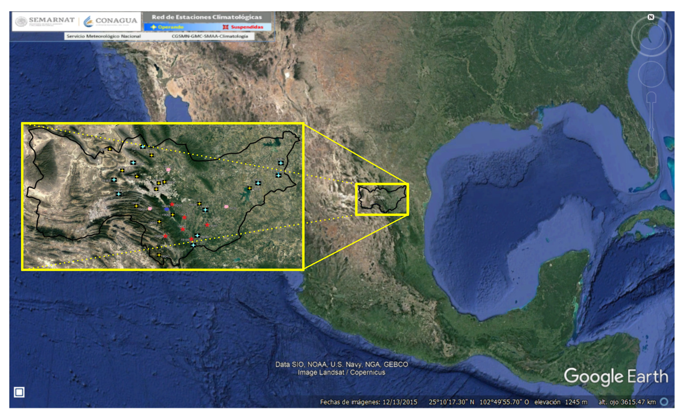
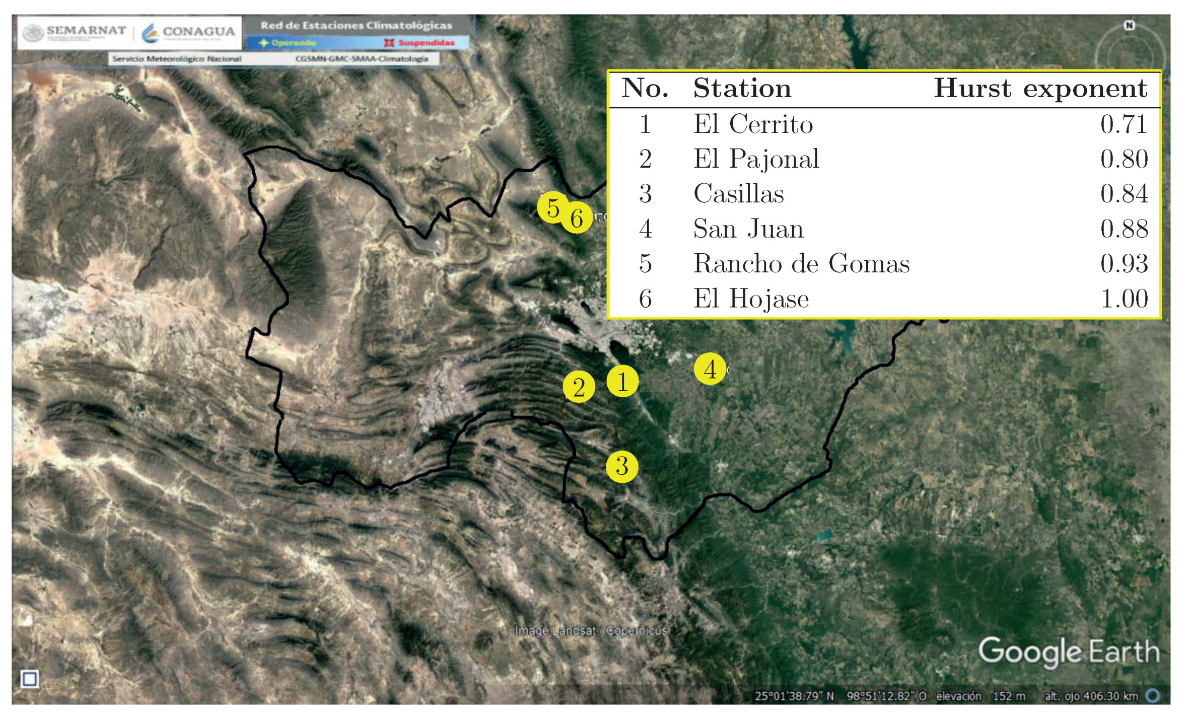
2.1. Data Acquisition

Our model was performed using actual data taken from Benavides-Bravo et al. (2015), a case study where clustering of rainfall stations in RH-24 Mexico Region was analyzed by utilizing data from the National Water Commission of Mexico (CONAGUA by its initials in Spanish), the institution responsible for water management in the country. That study was constructed using homogeneous sampling followed by a rigorous reliability process. There are several works where homogeneity is considered for rainfalls [30,31,32,33].

Based on the data obtained, assumed that from each rainfall cluster selected, the station corresponding to the median value of the Hurst exponent of such cluster was selected. The higher the station’s exponent, the greater the time series’ variability in long-term dependence (or persistence). Therefore, the selected stations represent the complete dataset from a mathematical point of view, which is the persistence of their corresponding time series. Moreover, the selected stations represent various elevations, since stations El Cerrito, El Pajonal and Casillas are located in the flanks of the Sierra Madre Oriental mountain chain. In contrast, San Juan, Rancho de Gomas and El Hojase are located in the valley of the basin. The selected stations are highlighted in Figure 2, indicating their corresponding Hurst exponent.

The time series used have different lengths depending on the records of their corresponding stations, so that the initial data were collected around the 1940–1960s, while all the series end in 2018. In turn, the data were recorded daily and averaged monthly. In this way, we considered an extensive and sufficient amount of data for each station (more than 720 data corresponding to 60 years) to characterize the variability of the mean rainfall.

2.2. Experimental Variograms

Let a rainfall time series $\{X_t,t\ge 0\}$ (in mm); we define the variogram $\gamma \left(h\right)$ as in [21,34] (they defined the variogram without the square root):

$$\gamma \left(h\right)=\sqrt{\frac{1}{2}Var\left[X(t+h)-X\left(t\right)\right]}=\sqrt{\frac{1}{2}E\left[{\left\{X(t+h)-X\left(t\right)\right\}}^2\right]},$$

(5)

where the square root is added with the aim of measuring our results in mm, which means half the variance of the difference between data is separated by an interval of time distance $\mathit{h}\in \mathbb{N}$ (expressed in months), which corresponds to half the expected square difference between those data. A table of symbols and units (

Table A1. Table of symbols and units.

Symbol	Name	Units
h	Lag distance	Months
$\gamma \left(h\right)$	Variogram	mm
c	Sill	mm
r	Maximal variability	Months
$c_{{}_0}$	nugget variance, nugget effect	mm${}^2$
a	distance parameter	Months
$\{X_t,t\ge 0\}$	time series	mm
$Var(·)$	Variance	mm${}^2$
$E(·)$	Expected value	mm
$n\left(h\right)$	number of differences with a lag of value h	Dimensionless
H	Maximum of $n\left(h\right)$	Dimensionless
$b_1$	Quadratic–exponential model coefficient	mm/month
$b_2$	Quadratic–exponential model coefficient	mm/month${}^2$
k	Quadratic–exponential model coefficient	Dimensionless
$r_{{}_0}$	The initial time distance	Months
$R^2$	Coefficient of determination	Dimensionless
$RMSE$	root mean square error	mm

) is included in Appendix A.

The scale is then defined by $\mathit{h}$; from the minimal distance value, increasing $\mathit{h}$ allows the quantitative representation of long-term variations in the hydrological series. A critical remark is that Equation (5) works on the average of the differences $\left(X\right(t+h)-X(t\left)\right)$, so that it only depends on the interval $\mathit{h}$. Consequently, for a given times series located at a fixed point in the space, the trend or the persistence of such series is only characterized by $\mathit{h}$.

Now, the discrete version of Equation (5) can be written as [34]:

$$\gamma \left(h\right)=\sqrt{\frac{1}{2n\left(h\right)}\sum _{t=1}^{n\left(h\right)}{(X(t+h)-X\left(t\right))}^2},$$

(6)

where $n\left(h\right)$ has dimensionless units and denotes the number of differences with a lag of value h. We applied Equation (6) to the selected rainfall stations mentioned in Section 2.1, using $h=1,2,\dots ,H$, where H months depends on the total length of the series. The generated variograms are shown in Figure 3; for a better illustration, variability is only shown up to the first 120 neighbors, i.e., regarding ten years of difference.

2.3. Curve Fitting

Due to the cyclical nature of the studied rainfall variograms, some extra steps must be completed to analyze the maximal variability:

(1)

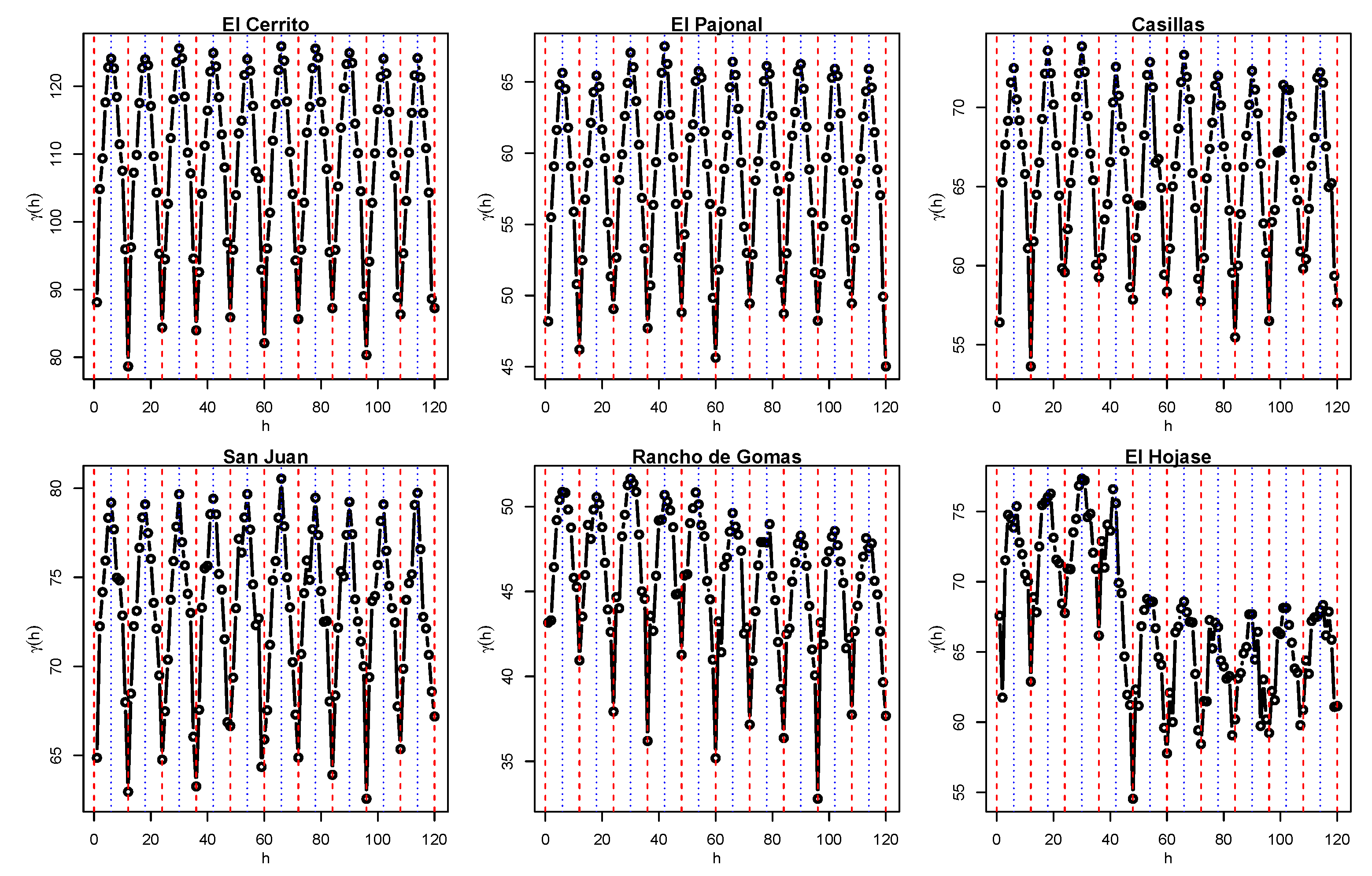
Division of the variogram. An inspection of the experimental variograms indicates that a similar pattern is repeated every 12 neighbors or units of distance, as shown in Figure 3, so that the event seems to have an annual periodicity, which, in turn, agrees with natural or empirical knowledge. In this way, the variogram for the complete series is calculated by Equation (6) and then divided into several variograms with a length of 12 months.

(2)

Average of the resulting variograms. The set of variograms obtained from Step (1) have a similar structure. On average, the curve increases until it reaches a maximal value at the sixth neighbor ($h=6$ months) and then decreases in a quasi-symmetrical way, as shown in Figure 3. Since the analysis of the maximum variability is the usual objective when studying variograms, and that the curve obtained might be considered as symmetric, we only focus on the first half of the variograms, i.e., from $h=1$ to $h=6$ months, where such values correspond to the position of the initial data ($r_0$) and the maximal variability (r), respectively, where months are the units for both cases. Then, the variograms of a station are averaged point by point to obtain a single curve that represents or characterizes such a station.

(3)

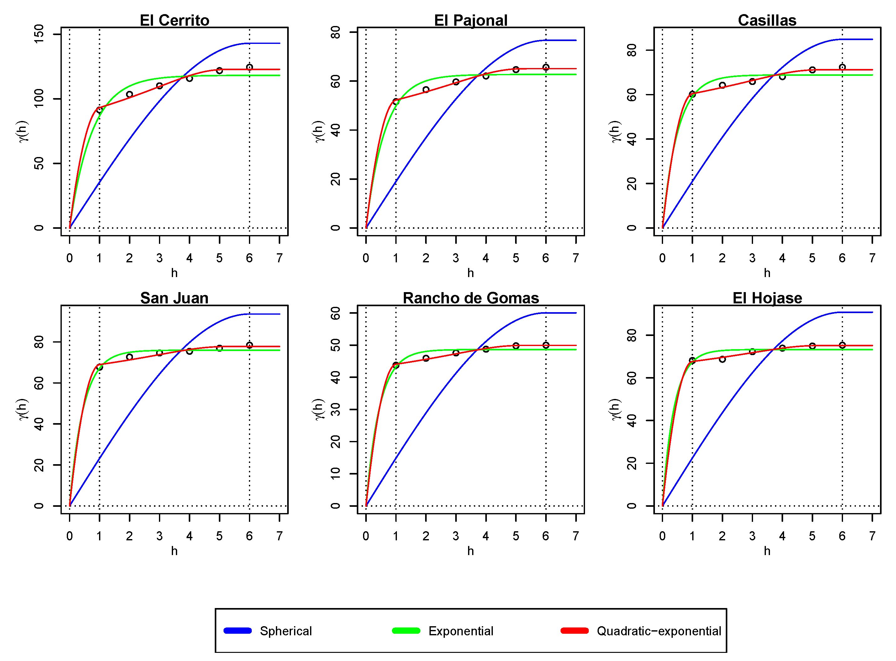
Fitting a model. A more detailed inspection of each averaged variogram suggests a curve that is concave downward in its entirety until it reaches a final sill, as shown in Figure 3. As mentioned in Section 1, this shape has the characteristics of the spherical and exponential models. We implemented such models and one more that we constructed to fit the variograms. The proposed model is described in the following subsection. This was the only step carried out by using the R statistics program [35]. All the previous steps (the processing of the data) were executed by using Microsoft Excel.

2.4. A Quadratic–Exponential Model

The model we propose originated from the formula of the exponential model (3) without the nugget effect. The main modification consists of guaranteeing that the variogram range has a value of r by modifying the argument of the exponential term, from $\left(e^{-\frac{\left|h\right|}{a}}\right)$ to $\left(e^{-\frac{\left|h\right|}{r-\left|h\right|}}\right)$. This change produces a continuous and differentiable model only up to the value of $\left|h\right|<r$. Therefore, the model must be defined as a piecewise function, with a constant value (the sill of the curve) of $\gamma \left(h\right)=c$, for $\left|h\right|\ge r$.

Then, the quadratic–exponential model is a three-piecewise function in which the nearest part to the origin consists of a quadratic expression, the middle part of an exponential expression, during the farthest part of a constant, so that:

$$\gamma \left(h\right)=\left\{\begin{array}{ccc}{b}_1{\left|h\right|}^2+b_2\left|h\right|& \mathrm{if}& 0\le \left|h\right|\le r_0\\ c\left(1-k{e}^{-\frac{\left|h\right|}{r-\left|h\right|}}\right)& \mathrm{if}& r_0\le \left|h\right|<r.\\ c& \mathrm{if}& \left|h\right|\ge r\end{array}\right.$$

(7)

In addition to the explanation provided for the second and third parts of Equation (7), $k\in \mathbb{R}:k\in [0,1]$ is introduced as a factor modifying the peak amplitude of the exponential term, such that $\left(\gamma \left(h\right)=c\left[1-k{e}^{-\frac{\left|h\right|}{r-\left|h\right|}}\right]\right)$. This means one more degree of freedom to modify the effect of the exponential term and, consequently, the slope of the curve. Moreover, it produces an automatic nugget effect in the variogram, since $k<1$. The second part starts at $r_0$, which we define as the initial time distance at which we gain our first datum, and it must satisfy $r_0>0$.

It is important to mention that the quadratic–exponential model is conditionally positive for all the $\left|h\right|$-values similar to the exponential model. In fact, this is the only necessary condition for Equation (7) to be considered as a variogram [21]. Additionally, the model is continuous and differentiable at $\left|h\right|=r$.

On the other hand, the first part of Equation (7) occurs from the distance $h=0$ to the initial data at $\left|h\right|=r_0$ and is defined by a quadratic expression. This part is added to eliminate the nugget effect from the model by a smoothing curve near to the origin. The coefficients $b_1$ and $b_2$ are obtained by satisfying the conditions of continuity, ${\gamma }_1\left(h\right)={\gamma }_2\left(h\right)$ and differentiability, ${\gamma }_1^{\prime }\left(h\right)={\gamma }_2^{\prime }\left(h\right)$ of the model at $\left|h\right|=r_0$.

Let ${\gamma }_1\left(h\right)=b_1{\left|h\right|}^2+b_2\left|h\right|$ and ${\gamma }_2\left(h\right)=c\left[1-k{e}^{-\frac{\left|h\right|}{r-\left|h\right|}}\right]$.

Then, at $\left|h\right|=r_0$, produces:

$$b_1=\frac{c}{{r_0}^2}\left[k{e}^{-\frac{r_0}{r-r_0}}\left(1+\frac{r_{0}r}{{(r-r_0)}^2}\right)-1\right]$$

and

$$b_2=\frac{c}{r_0}\left[2-k{e}^{-\frac{r_0}{r-r_0}}\left(\frac{r_{0}r}{{(r-r_0)}^2}+2\right)\right]$$

Consequently, Model (7) is continuous for $h\in \mathbb{R}$ and differentiable for $h\in \mathbb{R},h\notin \{0,r\}$. In turn, whether the parameters $r_0$ and r are established by previous knowledge of the data or be easily extracted from the variogram, the model would only require the adjustment of c and k to be completed.

Therefore, we can comment on two main physical advantages of the use of the quadratic–exponential model:

(1)

Its quadratic behavior is close to the origin, which allows a smooth increase different to the exponential behavior, leading to a shorter and a larger range. This behavior is characteristic of nested structures, which are sometimes seen in experimental variograms [22,36,37].

(2)

It is guaranteed to reach the sill at the maximal variability r, which contrasts with the exponential model, where the sill must be approximated or calculated from c, a and the curve fitting [36,38].

The nugget effect

The nugget effect is introduced in this model by removing the nearest part of the function and extending the domain of the middle part so that:

$$\gamma \left(h\right)=\left\{\begin{array}{ccc}c\left(1-k{e}^{-\frac{\left|h\right|}{r-\left|h\right|}}\right)& \mathrm{if}& 0\le \left|h\right|<r\\ c& \mathrm{if}& \left|h\right|\ge r.\end{array}\right.$$

(8)

In this manner, the value of $\gamma \left(h\right)$ at the origin is directly calculated from Equation (7), so that $c_0=\gamma \left(0\right)=c\left(1-k\right)$. So, despite the fact that the quadratic expression is eliminated from the model, this way of adding the nugget effect allows one to highlight two main characteristics:

(1)

The number of parameters to fit (c and k) does not increase. This contrasts with the common models, in which an extra-parameter must be fitted ($c_0$).

(2)

The number of parameters to know a priori is reduced since $r_0$ is not required. This also allows one to reduce the complexity of the model and the execution of the fitting.

3. Results

In order to prove our model for our case of study, we performed curve fitting for the variogram of each rainfall station. The spherical, exponential and quadratic–exponential models were implemented with ((1),(3),(7)) and without ((2),(4),(8)) the nugget effect. These results are shown in Section 3.1 and Section 3.2.

A total of 1000 adjustments were carried out to obtain curve fitting for a model applied to a specific rainfall station. Herein, each set of adjustments is called a “simulation”. For each simulation, the adjustment with the best fitting, in terms of the residual sum of squares, was chosen.

All the adjustments of each simulation were performed by the least-squares method (LSM) using the optim function of the R statistics program with the method L-BFGS-B, which consists of a limited-memory modification of the method BFGS quasi-Newton, also known as the Variable Metric Algorithm. The modification allows box constraints; each variable can be given a lower and/or upper bound. The optim function is inside the package Stats, which is installed by default in the R software [35].

All the adjustments were initialized with random initial values inside the lower and upper bounds allowed during the fitting, which were fixed according to

Table 1. Values of the lower and upper bounds for each parameter. The variable y refers to the recorded data of $\gamma \left(h\right)$. The lower bound of parameter c changes to zero when using Equations (2) and (4).

Parameter	Lower Bound	Upper Bound
c	0.5 $maxy$	2 $maxy$
$c_0$	0	$miny$
a	0.01	r
k	0.01	1

. The only exception was parameter c, whose lower bound changed to zero when the nugget effect was considered in the spherical (2) and exponential (4) models. This because the sill of the curve is ($c_0+c$) with the nugget effect. The maximal variability $r=6$ (in months) and the position of our first data $r_0=1$ (in months) was introduced as a known parameter.

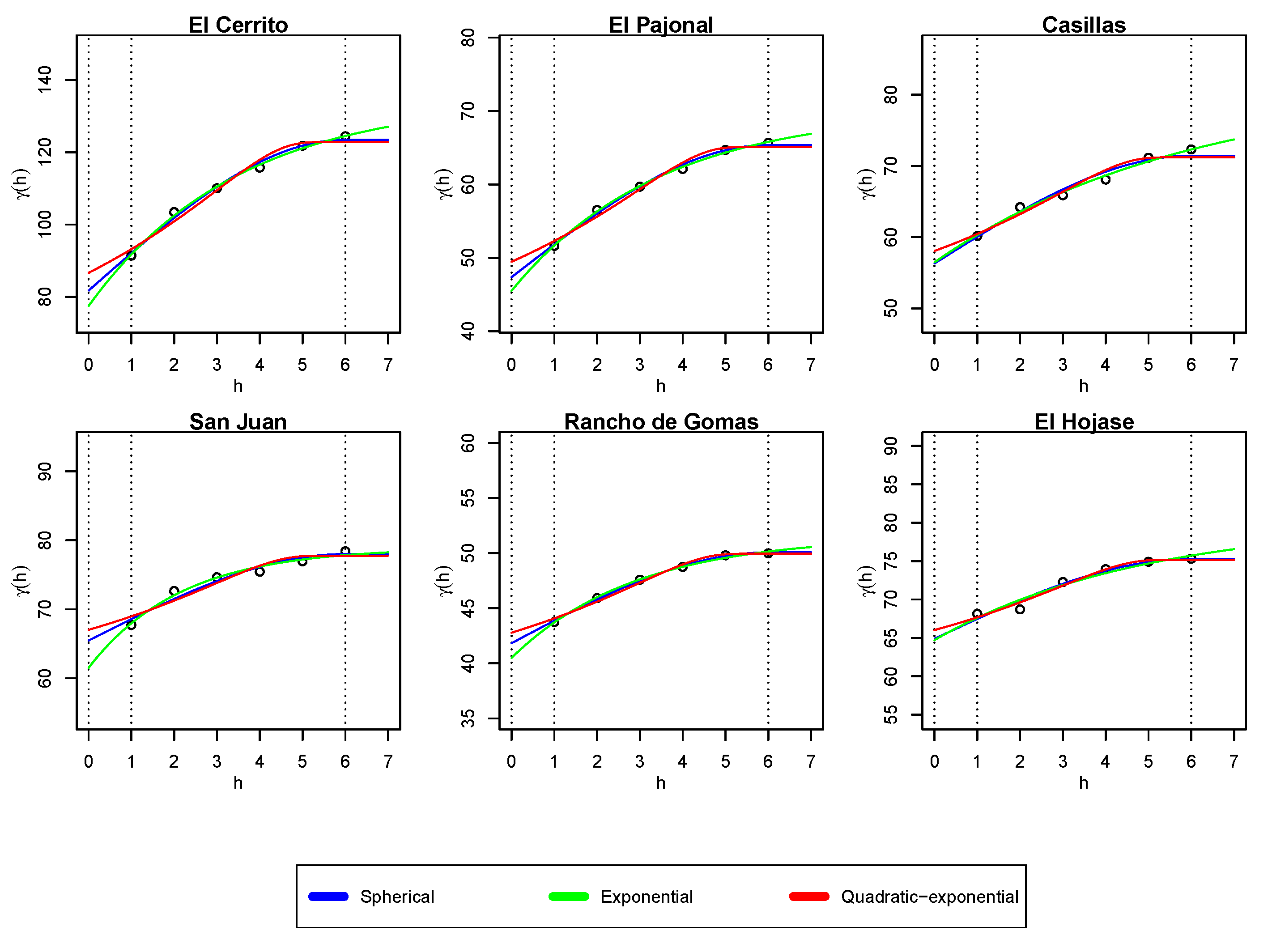
3.1. Fitting without the Nugget Effect

Figure 4 shows the best fitting obtained after a simulation with the spherical (1), exponential (3) and quadratic–exponential (7) models for each rainfall station. Despite our $y$—data decreasing after the maximal variability $r=6$ months, we plotted our models up the value of $h=7$ months to visualize those models’ behavior after r.

Table 2. Models’ parameters, coefficient of determination $R^2$ (dimensionless) and root-mean-square error ($RMSE$) (in mm) obtained by fitting each model to each station’s variogram.

Weather Station	Parameters			Coefficient of Determination	Error
Models	c	a	k	${\mathit{R}}^2$	$\mathit{RMSE}$
El Cerrito
Spherical	142.97	-	-	−5.678	29.13
Exponential	118.16	0.75	-	0.798	5.07
Quadratic–exponential	122.82	-	0.295	0.976	1.73
El Pajonal
Spherical	76.67	-	-	−11.103	16.87
Exponential	62.72	0.63	-	0.752	2.42
Quadratic–exponential	65.09	-	0.240	0.982	0.65
Casillas
Spherical	84.87	-	-	−22.650	20.07
Exponential	68.85	0.51	-	0.636	2.49
Quadratic–exponential	71.20	-	0.185	0.958	0.84
San Juan
Spherical	93.63	-	-	−44.648	23.33
Exponential	75.97	0.46	-	0.801	1.54
Quadratic–exponential	77.77	-	0.138	0.917	1.00
Rancho de Gomas
Spherical	60.05	-	-	−44.246	14.90
Exponential	48.64	0.45	-	0.698	1.22
Quadratic–exponential	49.94	-	0.143	0.988	0.24
El Hojase
Spherical	90.77	-	-	−64.823	16.88
Exponential	73.26	0.39	-	0.477	2.42
Quadratic–exponential	75.16	-	0.122	0.973	0.65

summarizes the results plotted in Figure 4. It shows the values obtained for the parameters of each model, namely a for the exponential model, k for the quadratic–exponential model, and c for all the models. In addition, the coefficient of determination $R^2\in (-\infty ,1]$ (dimensionless) [39,40], and the root-mean-square error $RMSE$ (mm) are reported for each simulation. Each measurement is shown with a different number of decimal digits, so that they all have (or produce) the same precision in terms of the amount of rain (in mm); namely, we selected a precision of ${10}^{-2}$ mm, which is 10 times more than the precision of the CONAGUA’s records [41]. The results for the stations are listed according to their Hurst exponent in ascending order.

3.2. Fitting with the Nugget Effect

Similarly to Figure 4, Figure 5 shows the best fitting obtained after a simulation for each rainfall station while considering the nugget effect. So, the curve fittings shown are those achieved when implementing Equations (2)—spherical, (4)—exponential and (8)—quadratic–exponential.

Table 3. Models’ parameters, coefficient of determination $R^2$ and root-mean-square error ($RMSE$), obtained by fitting each model to each station’s variogram, considering the nugget effect. Parameter a reached the maximal value allowed ($a=6$) in the exponential fitting for the station Casillas, as shown in Table 1.

Weather Station	Parameters				Coefficient of Determination	Error
Models	c	${\mathit{c}}_0$	a	k	${\mathit{R}}^2$	$\mathit{RMSE}$
El Cerrito
Spherical	41.76	81.70	-	-	0.992	1.03
Exponential	57.33	77.43	3.49	-	0.997	0.63
Quadratic–exponential	122.82	-	-	0.295	0.976	1.73
El Pajonal
Spherical	18.00	47.35	-	-	0.995	0.35
Exponential	24.66	45.50	3.47	-	0.998	0.22
Quadratic–exponential	65.09	-	-	0.240	0.982	0.65
Casillas
Spherical	15.12	56.31	-	-	0.969	0.73
Exponential	25.06	56.47	$6.00$	-	0.988	0.45
Quadratic–exponential	71.20	-	-	0.185	0.958	0.85
San Juan
Spherical	12.55	65.46	-	-	0.954	0.75
Exponential	17.44	61.50	2.16	-	0.981	0.48
Quadratic–exponential	77.77	-	-	0.138	0.917	1.00
Rancho de Gomas
Spherical	8.24	41.83	-	-	0.998	0.10
Exponential	11.05	40.49	2.90	-	0.997	0.12
Quadratic–exponential	49.94	-	-	0.143	0.988	0.24
El Hojase
Spherical	10.39	64.89	-	-	0.960	0.57
Exponential	15.46	64.72	4.83	-	0.949	0.64
Quadratic–exponential	75.16	-	-	0.122	0.973	0.47

summarizes the results plotted in Figure 5. It shows the values obtained for the parameters of each model, namely, c for all the models, a for the exponential model, k for the quadratic–exponential model, and $c_0$ for both of them. $R^2$ and $RMSE$ are also reported for each simulation. The results for the stations are listed according to their Hurst exponent in ascending order.

4. Discussion

4.1. Case Study

In a general way, results vary according to the type of fitting. Firstly, for all the simulations (for each station) without the nugget effect, the quadratic–exponential model has the best adjustment, which can be seen by the values of $R^2$ and $RMSE$ in Table 2 and even by a broad visualization of Figure 4. In detail, $R^2>0.95$ for all the rainfall stations (excepting for San Juan, $R^2=0.917$) when the quadratic–exponential model was applied (7), which corresponds to $RMSE$ values of less than 2 mm. In turn, these values indicate good precision for amount of rainfall per month; in addition, there is no dependence between the fit of the model and the Hurst exponent, so the model is robust in this sense. This contrasts with the spherical model (1), whose bad fitting is reflected in the negative values of $R^2$ and high values of $RMSE$ for all the stations; the larger the Hurst exponent, the worse the fitting. Exponential model (3) fits better for some stations than others, but there is no clear dependence on the Hurst number; its $R^2$-values are between 0.477 and 0.801, while $RMSE$ are between 1.22 and 5.07 mm, which is also acceptable. There is no clear relation between $R^2$ and $RMSE$ for all the models.

On the other hand, the spherical (2) and exponential models (4) greatly improved their fitting when considering the nugget effect. Namely, $R^2>0.95$ and $RMSE<1$ mm for practically all the stations when such models were applied, and there was not a clear dependence on the Hurst number. As the reader can see from Table 2 and Table 3, the results of the quadratic–exponential models are the same with (7) and without (8) the nugget effect, and this is because the fitting is the same. The only two parameters to fit in both versions are c and k, as mentioned in Section 2.4. Then, the same results are obtained because of the selection of the best fitting after the 1000 adjustments for both versions and the convergence of the optimizer used. The results for all the models are then excellent and similar for all the stations.

In this way, the quadratic–exponential model is the most robust of all the three, in the sense of maintaining a good fitting with different scenarios, such as analyzing time series with diverse Hurst numbers and/or requiring a fitting with or without the nugget effect. For example, we look for nugget effect behavior because the natural phenomenon we are considering is the average behavior of rainfall over the years, and there is variability in rain year by year (with 12th neighbors), as illustrated in Figure 3. Outside of the subject of rainfall, other examples of natural and artificial causes of a nugget effect can be found in [42].

We carried out simulations without considering the nugget effect to express that there could be some phenomena in which our initial data are not at $h=0$ but at $h=r_0$, and we do not know the physical behavior of the phenomenon close to the origin. In those situations, the quadratic–exponential model becomes a powerful tool. Furthermore, the quadratic behavior close to the origin gives our model the advantage of a smooth increase until it reaches the apparent nugget $c_0$ about the distance $r_0$, which is characteristic of phenomena with nested structures [22,36].

Now, the best results are also reflected in some parameters fitted. For the approximations without the nugget effect, c is larger but closer to the sill with the quadratic–exponential model than with the exponential model; in turn, c is much larger than the apparent sill of the curve when applying the spherical model. For the nugget effect, this is not clear, since the nugget $c_0$ takes an important role. From Figure 5, the quadratic–exponential model brings the most significant nugget than the spherical model, and finally the exponential model for almost all the stations, which is inversely related with $R^2$’s values and does not have relation with $RMSE$’s values; in fact, the exponential model gave the lowest values of $RMSE$ for four stations.

The sill (the sill is $c+c_0$ for the spherical and exponential models, and c for the quadratic–exponential model, as shown in Table 3) does not have a direct relation with the quality of the fitting. The only point to mention regarding it is that it is guaranteed to be reached at $h=6$ months in the spherical and quadratic–exponential models, while it is fitted in the exponential models by means of a. This causes contrast between the cases with and without the nugget effect when applying the last model because the sill is apparently reached for the first case before r (values of a between 0.39 and 0.75 months), while the curve continuously increases after r for the second case (values of a about 2.15 and 6.00 months). This also contrasts with quadratic–exponential behavior, where the value of k remains constant for both cases.

The parameter k decreases when the Hurst number increases, as seen in Table 2 and Table 3 throughout the stations. This behavior is also seen in a without considering the nugget effect, but it is not shown when the nugget is considered. This is because of the importance of $c_0$. This observation is highlighted in this paper, but its importance and possible reasons for its occurrence are left as a direction for future research. In addition, the difference between minimal and maximal variability for each station diminishes from ≈35 mm to ≈5 mm when the Hurst exponent increases. This is a critical point regarding the RH-24 region that could be connected with the parameter k in a future research.

Finally, all these results and observations highlight the advantages of performing curve fittings with the quadratic–exponential model when the maximal variability is known, which is possible because of the construction of the model. On the other hand, our study presented some limitations, namely: although our model was sufficiently validated, its row dataset presents a limited quantity of data for its analysis, which includes the handling of monthly time series instead of daily; therefore, the minimal variance comparison is of $h=1$ month. Consequently, we identified the following trends for future research: expanding our model to the spatial dimension for kriging applications; proving the applicability of the model in other topics such as those ones mentioned in Section 1; and extending the study area to cover the entire RH-24 region, which could be of great benefit in characterizing climate studies, as well as for agriculture and landslide risk purposes in the region.

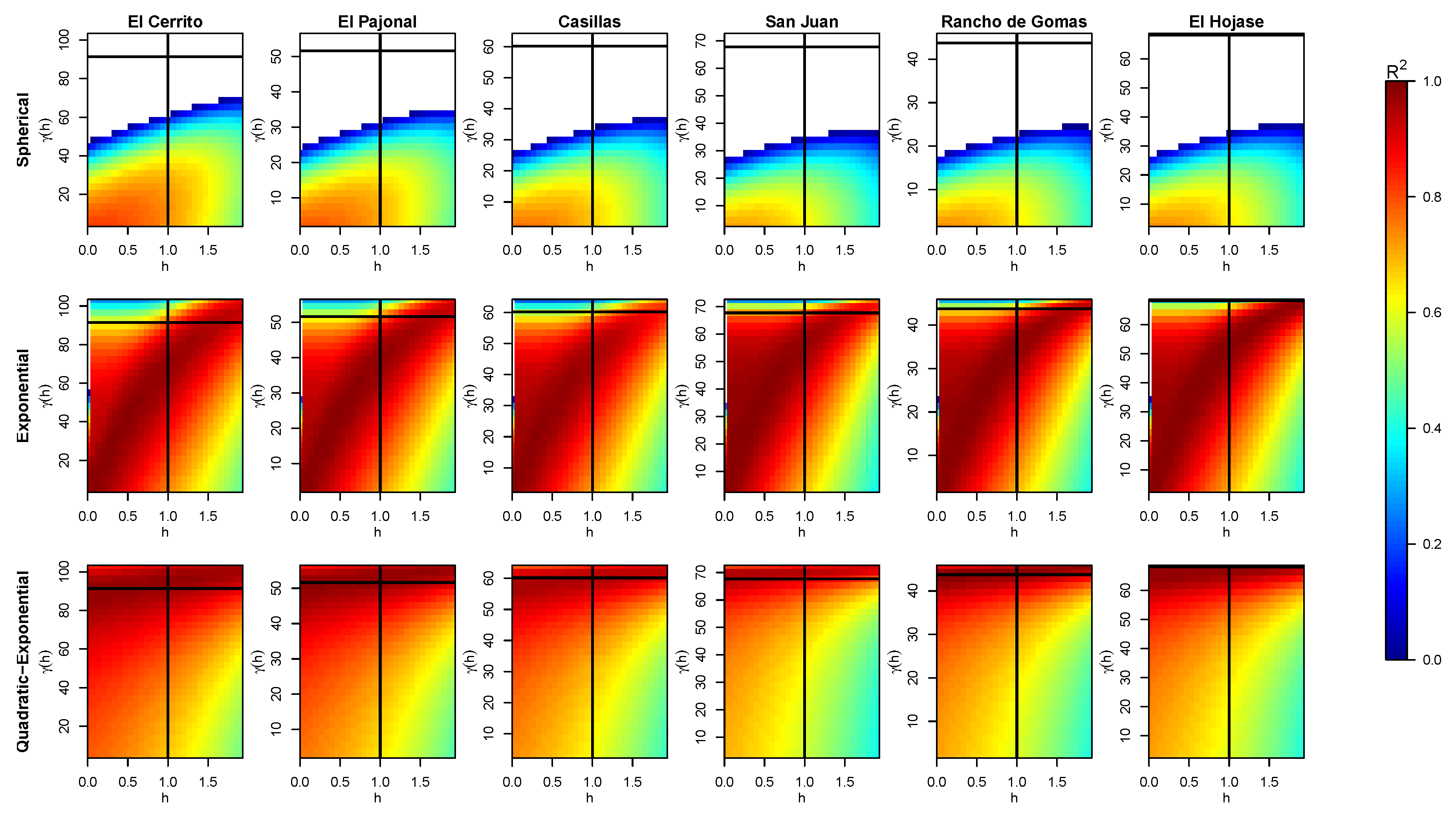
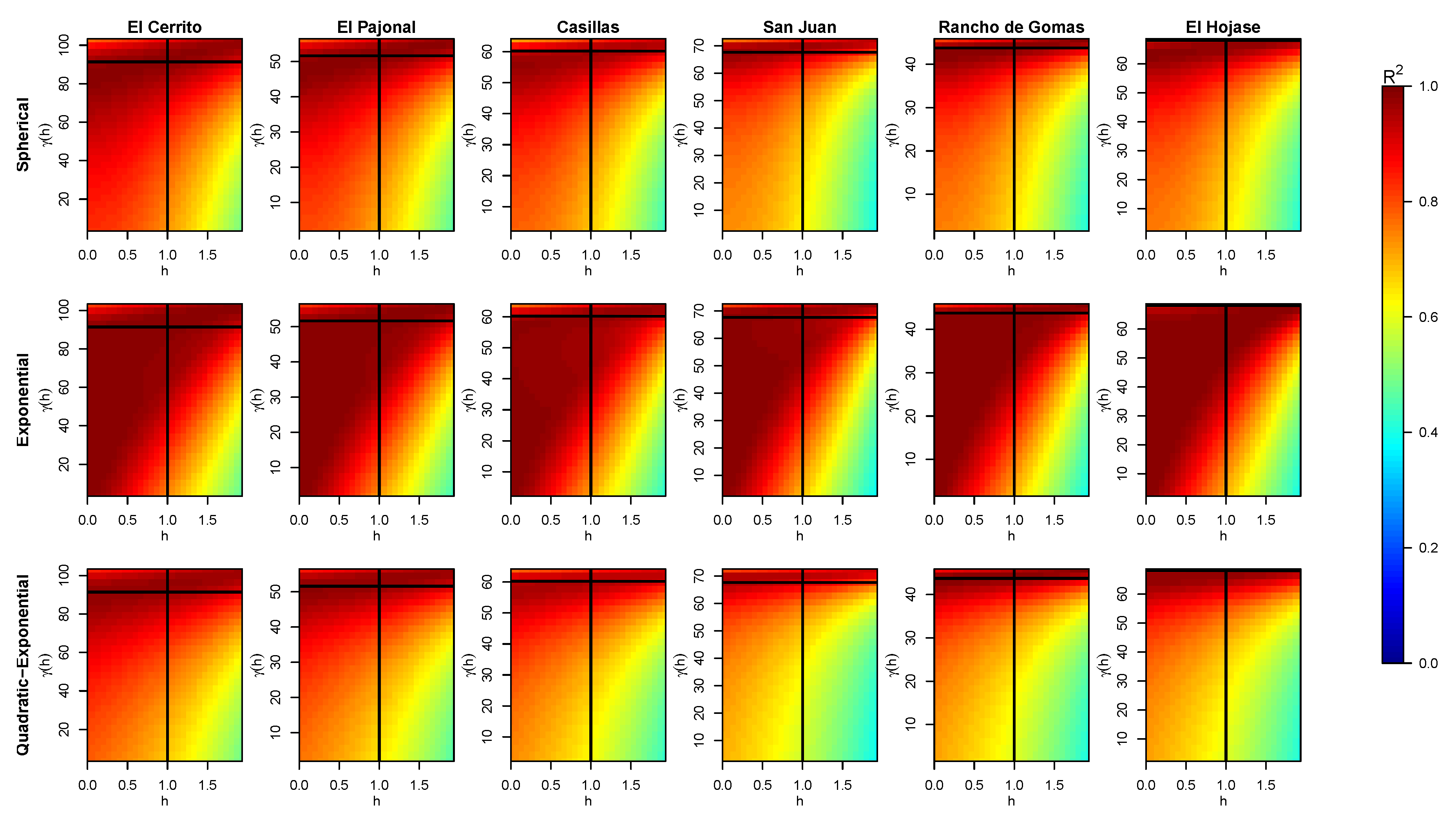
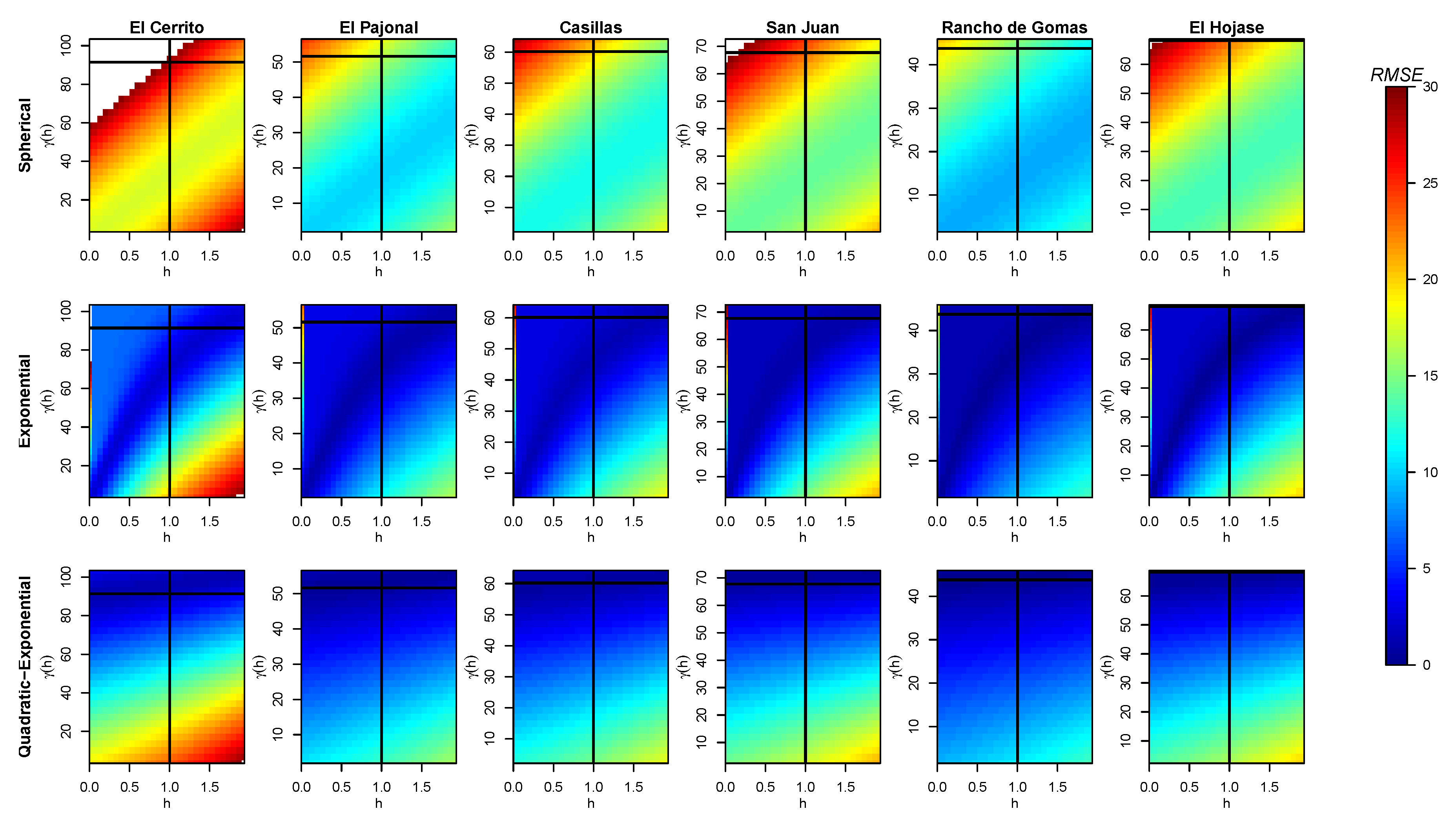
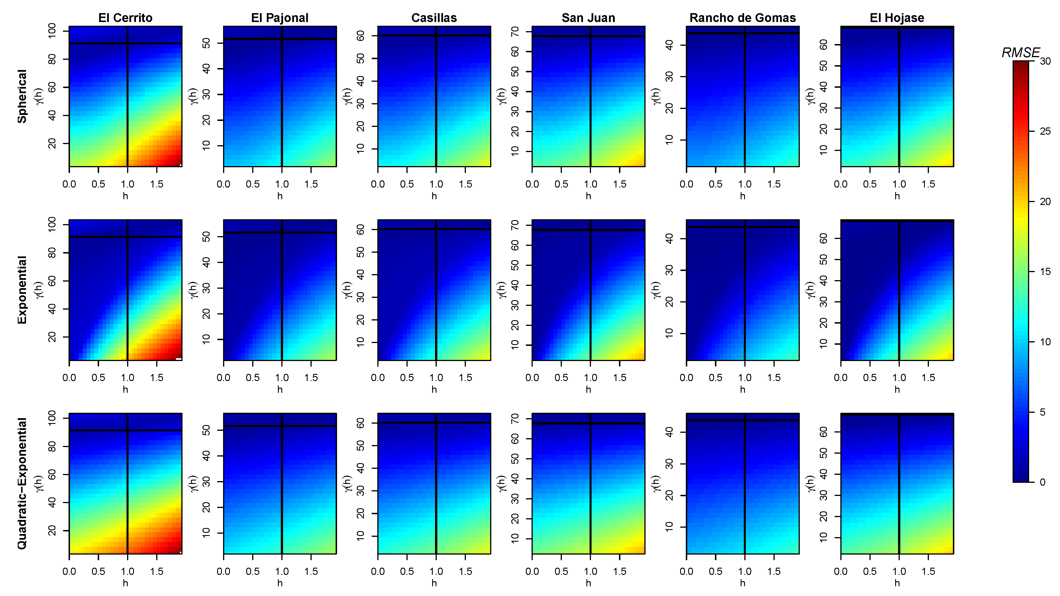
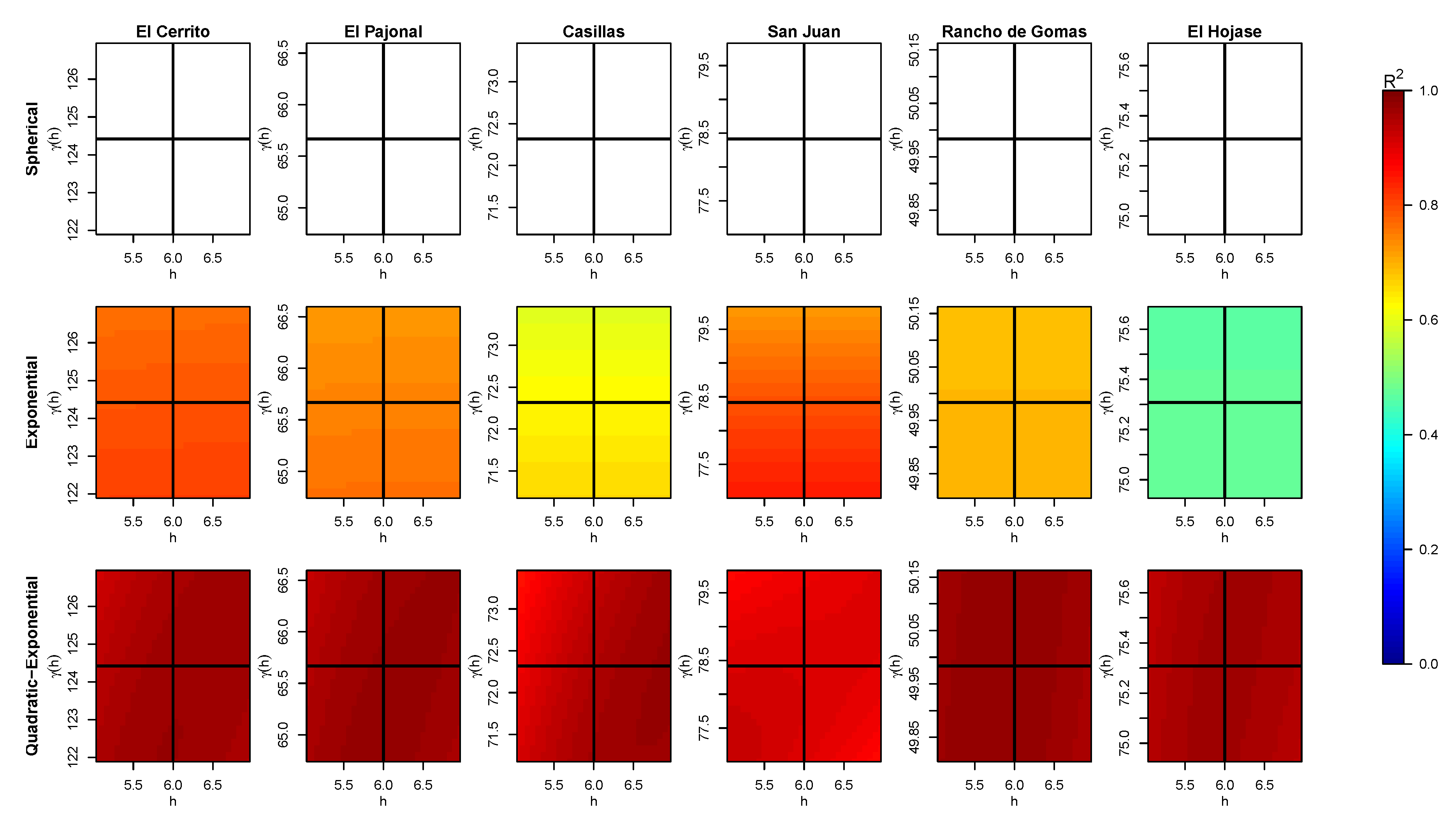
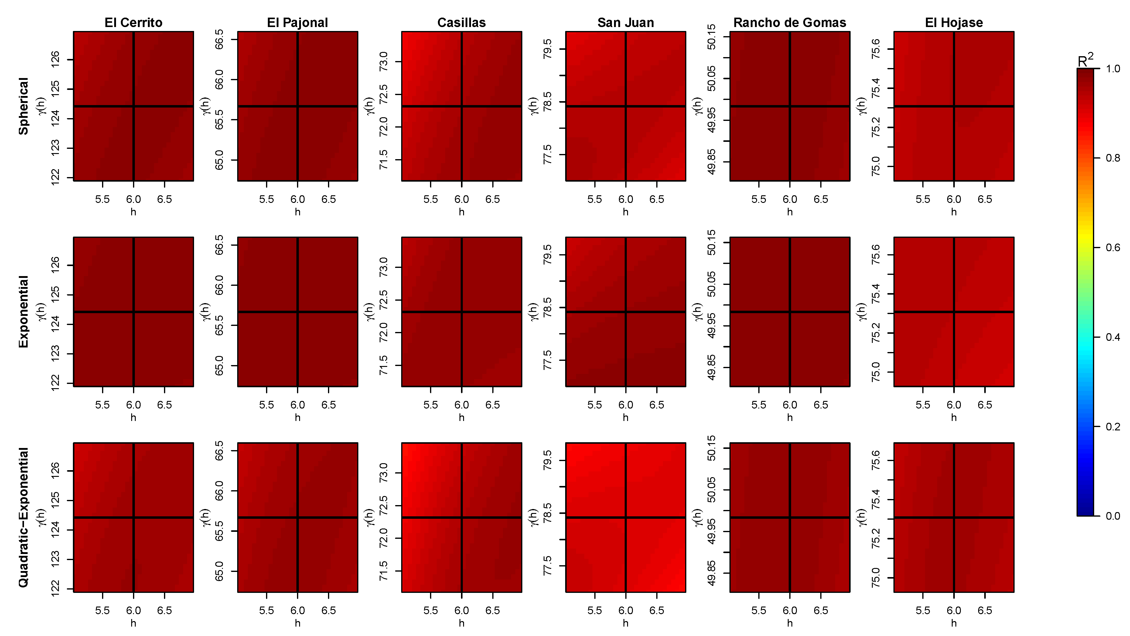
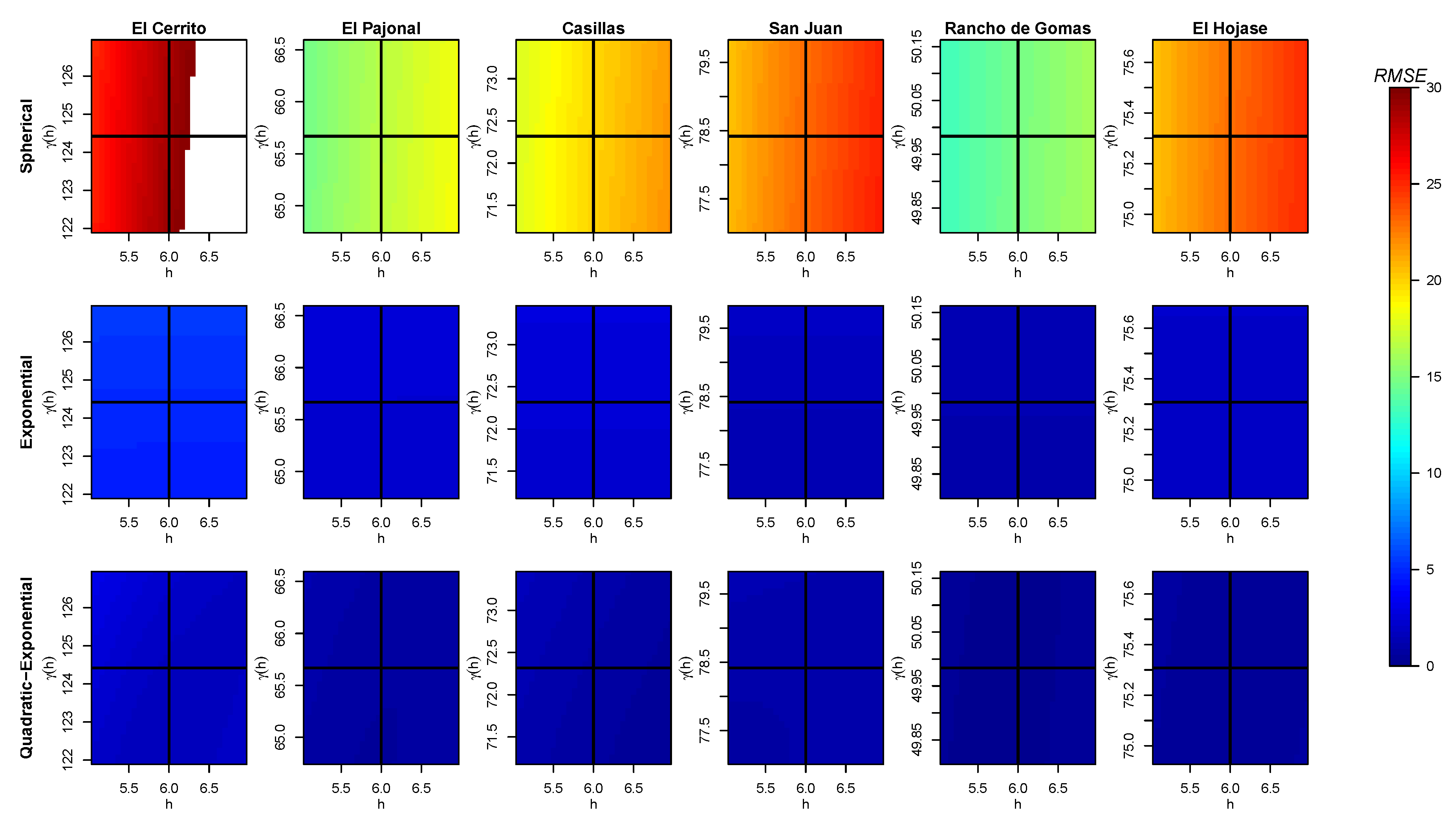
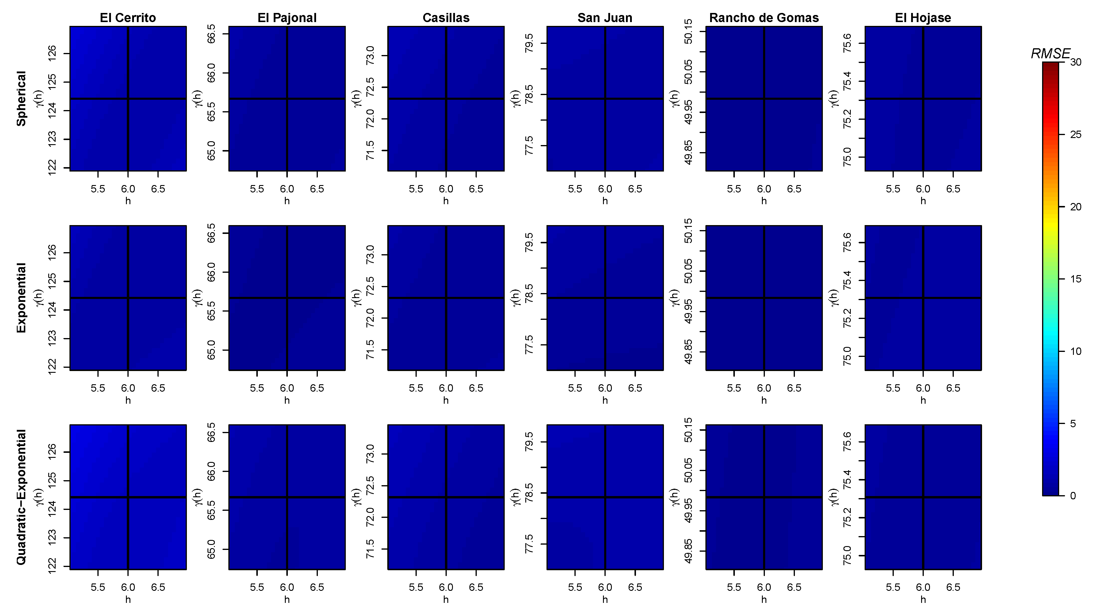
4.2. Numerical Analysis

With the aim of validating the results of the models in different scenarios, we carried out a numerical analysis that consisted of varying the values of the initial time distance $r_0$ and the maximal variability r. In detail, for the $r_0$’s analysis, we varied $r_0\in [0,2)$ and $\gamma \left(r_0\right)\in (0,\gamma \left(r_1\right)]$, where $\gamma \left(r_1\right)$ is our second datum of the experimental variogram. In turn, for the r’s analysis, we varied $r\in (r_4,2r-r_4)$ and $\gamma \left(r\right)\in (\gamma \left(r_4\right),\gamma (2r-r_4))$, as shown in Figure 6, Figure 7, Figure 8 and Figure 9, and in Figure A1, Figure A2, Figure A3 and Figure A4 of Appendix B, respectively.

For simulations without considering the nugget effect, Figure 6 shows how $R^2$ changes in a different way when using a different model. Namely, the spherical model improves its solution when $R_0\equiv (r_0,\gamma \left(r_0\right))$, close to the origin (left-down corner) in an apparent rotated elliptic behavior, for all the stations. In turn, the exponential model brings better solutions when $R_0$ moves through a curve going from the left-down to the right-up corner. These values are much better in the quadratic–exponential model, which provides its best solutions when $R_0$ is in the up-side, i.e., for high values of $\gamma \left(r_0\right)$. If the point $R_0$ is moved from its real position (the intersection of black lines in pictures), the exponential and quadratic–exponential models continue to provide the best solutions, but the exponential is better when both $r_0$ and $\gamma \left(r_0\right)$ have intermediate values, while the quadratic–exponential model is better when $\gamma \left(r_0\right)$ is higher, independently of $r_0$; however, it brings acceptable solutions for lower values of both $r_0$ and $\gamma \left(r_0\right)$. The fact that worse solutions are found at higher values of $r_0$ and lower values of $\gamma \left(r_0\right)$ for the latter models is easy to see, due to the behavior of the exponential and quadratic functions near to the origin, as defined in Equations (3) and (7), respectively.

In addition, $R^2$’s behavior changes when considering a nugget effect for the spherical and exponential models, as shown in Figure 7. Namely, for the exponential model, the left-up corner (low values of $r_0$ and high values of $\gamma \left(r_0\right)$) provides results similar to the best mentioned without the nugget effect. This is a direct consequence of the nugget effect. In turn, the spherical model provides very similar results to the quadratic–exponential model. All of this reflects the robustness of both models, exponential and ours, when data are noised or when they must fit to a specific behavior (considering or not considering the nugget effect). Specifically, the exponential model is better for values of $\gamma \left(r_0\right)$ directly proportional to $r_0$, whereas our model is better for high values of $\gamma \left(r_0\right)$, i.e., values near to $\gamma \left(r_1\right)$, where $r_1$ is the time distance of the next data. Thus, this suggests that our model is useful for such cases with high values of $\gamma \left(r_0\right)$, in which the spherical and exponential model do not fit well.

Now, $RMSE$’s results are very similar to $R^2$’s results, in qualitative terms, for the exponential and quadratic–exponential models. In Figure 8, the same patterns of $R^2$ are obtained for both models with a little variation throughout the stations, obtaining values of $RMSE$ lower than 5–7 mm for the up-side of our model and also for the left-down corner of the exponential model. The values of the exponential model improve when adding the nugget effect, as shown in Figure 9. Only some points $(h,\gamma (h\left)\right)$ of the right-bottom corner in pictures of both models are higher than an $RMSE$ of 25 mm.

On the other hand, the spherical model changes its elliptic behavior when $R^2$ does not have the nugget effect for a linear behavior, with its best $RMSE$’s values on the corresponding straight line and the worst solutions in the left-up and right-down corners. Then, similarly to $R^2$, it greatly improves its results when adding the nugget effect, namely, its results are similar to those ones of our model.

Finally, we found only small differences between results when varying the maximal variability r for $R^2$ and $RMSE$. The most significant of them is a low positive gradient of $RMSE$’s results when h is increased; for the spherical model without considering the nugget effect, see Figure A3. We did not perform a discussion about it due to the the low significance of the results. They are shown in Figure A1, Figure A2, Figure A3 and Figure A4 of Appendix B.

5. Conclusions

• Modeling spatial or temporal variation of data by an appropriate variogram is crucial for kriging interpretation, especially for small samples such as in our case study.
• We constructed a piecewise model of variogram, which is helpful in analyzing time series with few data, the monthly-accumulated value of a significant rainfall dataset. The model consists of a variation of the exponential model but introduces the maximal variability directly in the formula and adds a quadratic behavior near to the origin to obtain a continuous model from the origin.
• Compared with the spherical and exponential models, the “quadratic–exponential model” is the most robust, in the sense of fitting better without the nugget effect and providing good results without a significant difference between the other models when considering such an effect. In addition, it provided good results for time series with different Hurst numbers for our case study: rainfall in the RH-24 Mexico Region.
• Moreover, parameters to be fitted with that model are the sill c and the amplitude of the exponential term k, despite the nugget, regardless of whether or not the nugget is considered. So, the number of parameters does not increase with the nugget effect.
• In this way, our model results suggest that it could be a powerful tool when analyzing rainfall or other time/spatial series. Furthermore, the procedure we introduced in our methodology completes the steps for analyzing rainfall time series, from constructing the experimental variogram to fit a suitable model for the data.
• Additionally, a numerical analysis was performed to prove the robustness of the quadratic–exponential model. After a comparison against our control models, we can conclude that, for purposes with similar factors considered in this study, the quadratic–exponential model is sufficiently robust for any application where control models are utilized, and provides better results than those models for specific cases with high values of $\gamma \left(r_0\right)$.

References

1. Cerón, W.L.; Andreoli, R.V.; Kayano, M.T.; Canchala, T.; Carvajal-Escobar, Y.; Souza, R.A.F. Comparison of spatial interpolation methods for annual and seasonal rainfall in two hotspots of biodiversity in South America. An. Acad. Bras. Ciências [Online] 2021, 91. [Google Scholar] [CrossRef]
2. Gutiérrez-López, A.; Ramirez, A.; Lebel, A.I.; Santillán, T.; Carlos, O.F. El variograma y el correlograma, dos estimadores de la variabilidad de mediciones hidrológicas. Rev. Fac. Ing. Univ. Antioq. 2011, 59, 193–202. [Google Scholar]
3. Ly, S.; Charles, C.; Degré, A. Geostatistical interpolation of daily rainfall at catchment scale: The use of several variogram models in the Ourthe and Ambleve catchments, Belgium. Hydrol. Earth Syst. Sci. 2011, 15, 2259–2274. [Google Scholar] [CrossRef] [Green Version]
4. Muhamad Ali, M.Z.; Othman, F. Selection of variogram model for spatial rainfall mapping using analytical hierarchy procedure (AHP). Sci. Iran. 2017, 24, 28–39. [Google Scholar] [CrossRef] [Green Version]
5. Deutsch, C.V. Geostatistics. In Encyclopedia of Physical Science and Technology, 3rd ed.; Meyers, R.A., Ed.; Academic Press: New York, NY, USA, 2003; pp. 697–707. [Google Scholar] [CrossRef]
6. Díaz, M. Geoestadística Aplicada. 2002. Available online: http://www.esmg-mx.org/media/courses/geoestadistica/GeoEstadistica.pdf (accessed on 1 September 2021).
7. Samui, P.; Bui, D.T. Handbook of Probabilistic Models; Elsevier: Amsterdam, The Netherlands, 2020. [Google Scholar] [CrossRef]
8. Webster, R.; Oliver, M. How large a sample is needed to estimate the regional variogram adequately? In Geostatistics Tróia ’92. Quantitative Geology and Geostatistics; Springer: Dordrecht, The Netherlands, 1993; pp. 155–166. [Google Scholar] [CrossRef]
9. Kalauzi, A.; Čukić, M.; Millán, H.; Bonafoni, S.; Biondi, R. Comparison of fractal dimension oscillations and trends of rainfall data from Pastaza Province, Ecuador and Veneto, Italy. Atmos. Res. 2009, 93, 673–679. [Google Scholar] [CrossRef]
10. I. Negrón Juárez, R.; T. Liu, W. FFT analysis on NDVI annual cycle and climatic regionality in Northeast Brazil. Int. J. Climatol. 2001, 21, 1803–1820. [Google Scholar] [CrossRef]
11. Jeannée, N.; Nedellec, V.; Bouallala, S.; Deraisme, J.; Desqueyroux, H. Geostatistical assessment of long term human exposure to air pollution. In Geostatistics for Environmental Applications; Springer: Berlin/Heidelberg, Germany, 2005; pp. 161–172. [Google Scholar]
12. Marwanza, I.; Azizi, M.A.; Nas, C.; Anugrahadi, A.; Dahani, W.; Subandrio, S.; Salim, D.K.; Prima, A. The determination of information point distribution and classfication of confidence level estimation of geotechnic solid rock kriging estimation parameter based on variogram analysis. AIP Conf. Proc. 2020, 2267, 020040. [Google Scholar] [CrossRef]
13. Oliver, M.A.; Webster, R. Basic Steps in Geostatistics: The Variogram and Kriging; SpringerBriefs in Agriculture, Springer: Berlin/Heidelberg, Germany, 2015. [Google Scholar]
14. Myers, D.E.; Begovich, C.L.; Butz, T.R.; Kane, V.E. Variogram models for regional groundwater geochemical data. J. Int. Assoc. Math. Geol. 1982, 14, 629–644. [Google Scholar] [CrossRef]
15. Menezes, R.; Garcia-Soidán, P.; Febrero-Bande, M. A comparison of approaches for valid variogram achievement. Comput. Stat. 2005, 20, 623–642. [Google Scholar] [CrossRef] [Green Version]
16. Mahdi, E.; Abuzaid, A.H.; Atta, A.M. Empirical variogram for achieving the best valid variogram. Commun. Stat. Appl. Methods 2000, 27, 547–568. [Google Scholar] [CrossRef]
17. Cressie, N. Fitting variogram models by weighted least squares. J. Int. Assoc. Math. Geol. 1985, 17, 563–586. [Google Scholar] [CrossRef]
18. Adhikari, K.; Smith, D.R.; Collins, H.; Haney, R.L.; Wolfe, J.E. Corn response to selected soil health indicators in a Texas drought. Ecol. Indic. 2021, 125, 107482. [Google Scholar] [CrossRef]
19. Ali, G.; Sajjad, M.; Kanwal, S.; Xiao, T.; Khalid, S.; Shoaib, F.; Gul, H.N. Spatial–temporal characterization of rainfall in Pakistan during the past half-century (1961–2020). Sci. Rep. 2021, 11, 1–15. [Google Scholar] [CrossRef]
20. Somayasa, W.; Sutiari, D.K.; Sutisna, W. Optimal prediction in isotropic spatial process under spherical type variogram model with application to corn plant data. J. Phys. Conf. Ser. 2021, 1940, 012003. [Google Scholar] [CrossRef]
21. Chilès, J.; Delfiner, P. Geostatistics: Modeling Spatial Uncertainty; Wiley Series in Probability and Statistics; Wiley: Hoboken, NJ, USA, 2012. [Google Scholar]
22. Armstrong, M. Basic Linear Geostatistics; Springer: Berlin/Heidelberg, Germany, 1988. [Google Scholar] [CrossRef]
23. Camana, F.; Deutsch, C. Geostatistics Lessons. 2021. Available online: http://geostatisticslessons.com/lessons/nuggeteffect (accessed on 1 September 2021).
24. Garrigues, S.; Allard, D.; Baret, F.; Weiss, M. Quantifying spatial heterogeneity at the landscape scale using variogram models. Remote Sens. Environ. 2006, 103, 81–96. [Google Scholar] [CrossRef]
25. Sanchez-Castillo, L.; Kubota, T.; Cantú-Silva, I.; Moriyama, T. A probability method of rainfall warning for sediment-related disaster in developing countries: A case study in Sierra Madre Oriental, Mexico. Nat. Hazards 2016, 85, 1893–1906. [Google Scholar] [CrossRef]
26. Motalvo-Arrieta, J.; Chávez-Cabello, G.; Velasco-Tapia, F.; de León I., N. Causes and effects of landslides in Monterrey Metropolitan Area, NE Mexico. In Landslides: Causes, Types; Nova Science Publishers: New York, NY, USA, 2010; pp. 73–104. [Google Scholar]
27. Salinas-Jasso, J.A.; Velasco-Tapia, F.; Navarro de León, I.; Salinas-Jasso, R.A.; Alva-Niño, E. Estimation of rainfall thresholds for shallow landslides in the Sierra Madre Oriental, northeastern Mexico. J. Mt. Sci. 2020, 17, 1565–1580. [Google Scholar] [CrossRef]
28. Salinas-Jasso, J.; Salinas-Jasso, R.; Montalvo-Arrieta, J.; Alva-Niño, E. Inventario de movimientos en masa en el sector sur de la Saliente de Monterrey. Caso de estudio: Cañón Santa Rosa, Nuevo León, noreste de México. Rev. Mex. Cienc. Geol. 2017, 34, 182–198. [Google Scholar] [CrossRef] [Green Version]
29. Villarreal-Macés, S.G.; Díaz-Viera, M.A. Geostatistical estimation of the spatial distribution of mean monthly and mean annual rainfall in Nuevo León, Mexico (1930–2014). Tecnol. Cienc. Del Agua 2018, 9, 106–130. [Google Scholar] [CrossRef]
30. Caloiero, T.; Filice, E.; Coscarelli, R.; Pellicone, G. A Homogeneous Dataset for Rainfall Trend Analysis in the Calabria Region (Southern Italy). Water 2020, 12, 2541. [Google Scholar] [CrossRef]
31. Ahmed, K.; Shahid, S.; Ismail, T.; Nawaz, N.; Wang, X.J.; Ahmed, K.; Shahid, S.; Ismail, T.; Nawaz, N.; Wang, X.J. Absolute homogeneity assessment of precipitation time series in an arid region of Pakistan. Atmósfera 2018, 31, 301–316. [Google Scholar] [CrossRef]
32. Ros, F.C.; Tosaka, H.; Sidek, L.M.; Basri, H. Homogeneity and trends in long-term rainfall data, Kelantan River Basin, Malaysia. Int. J. River Basin Manag. 2016, 14, 151–163. [Google Scholar] [CrossRef]
33. Agha, O.M.A.M.; Çağatay Bağçacı, S.; Şarlak, N. Homogeneity Analysis of Precipitation Series in North Iraq. IOSR J. Appl. Geol. Geophys. 2017, 05, 57–63. [Google Scholar] [CrossRef]
34. Benavides-Bravo, F.G.; Almaguer, F.J.; Soto-Villalobos, R.; Tercero-Gómez, V.; Morales-Castillo, J. Clustering of Rainfall Stations in RH-24 Mexico Region Using the Hurst Exponent in Semivariograms. Math. Probl. Eng. 2015, 2015, 1–7. [Google Scholar] [CrossRef] [Green Version]
35. R Core Team. R: A Language and Environment for Statistical Computing; R Foundation for Statistical Computing: Vienna, Austria, 2020. [Google Scholar]
36. Webster, R.; Stewart, B.A. Quantitative Spatial Analysis of Soil in the Field. In Advances in Soil Science; Springer: Dordrecht, The Netherlands, 1985; pp. 1–70. [Google Scholar] [CrossRef]
37. Myers, D.E.; Journel, A. Variograms with zonal anisotropies and noninvertible kriging systems. Math. Geol. 1990, 22, 779–785. [Google Scholar] [CrossRef]
38. Wang, J.; Fu, B.; Qiu, Y.; Chen, L.; Wang, Z. Geostatistical analysis of soil moisture variability on Da Nangou catchment of the loess plateau, China. Environ. Geol. 2001, 41, 113–120. [Google Scholar] [CrossRef] [Green Version]
39. Barrett, J.P. The Coefficient of Determination—Some Limitations. Am. Stat. 1974, 28, 19–20. [Google Scholar] [CrossRef]
40. Saunders, L.J.; Russell, R.A.; Crabb, D.P. The Coefficient of Determination: What Determines a Useful R2 Statistic? Investig. Ophthalmol. Vis. Sci. 2012, 53, 6830–6832. [Google Scholar] [CrossRef] [Green Version]
41. Monthly Summaries of Temperatures and Rain. Available online: https://smn.conagua.gob.mx/es/climatologia/temperaturas-y-lluvias/resumenes-mensuales-de-temperaturas-y-lluvias (accessed on 17 September 2021).
42. Carrasco, P. Nugget effect, artificial or natural? The J. South. Afr. Inst. Min. Metall. 2010, 10, 299–305. [Google Scholar]
Figure 1. Location of the RH-24 México region.
Mathematics 09 02466 g001
Figure 2. Selected stations and their Hurst exponents.
Mathematics 09 02466 g002
Figure 3. Experimental variograms for each rainfall station until ten years of difference, h = 120 . Red dashed lines tag variability at 0 , 12 , 24 , , 120 months, while blue dotted lines tag variability at 6 , 18 , 30 , , 114 months.
Mathematics 09 02466 g003
Figure 4. Curve fitting for each station’s variogram with the spherical (1), exponential (3) and quadratic–exponential (7) models. The initial time distance r 0 = 1 month and the maximal variability r = 6 months are tagged with dotted lines.
Mathematics 09 02466 g004
Figure 5. Curve fitting for each station’s variogram with the spherical (2), exponential (4) and quadratic–exponential (8) models. The fitting is carried out considering the corresponding models with the nugget effect. The initial time distance r 0 = 1 month and the maximal variability r = 6 months are tagged with dotted lines.
Mathematics 09 02466 g005
Figure 6. Obtained values of R 2 (color bar) for different pair of data R 0 = ( r 0 , γ ( r 0 ) ) when fitting a curve for the variogram of each station with the three models and without considering the nugget effect. The intersection of the black solid lines tags the real R 0 in our experimental variogram. The white areas (in the results of the spherical model) correspond to lower values than those shown on the color scale, i.e., lower than zero.
Mathematics 09 02466 g006
Figure 7. Obtained values of R 2 (color bar) for different pair of data ( r 0 , γ ( r 0 ) ) when fitting a curve for the variogram of each station with the three models and considering the nugget effect. The intersection of the black solid lines tags the real R 0 .
Mathematics 09 02466 g007
Figure 8. Obtained values of R M S E (color bar) for different pair of data ( r 0 , γ ( r 0 ) ) when fitting a curve for the variogram of each station with the three models and without considering the nugget effect. The intersection of the black solid lines tags the real R 0 . The white areas correspond to higher values than those shown on the color scale.
Mathematics 09 02466 g008
Figure 9. Obtained values of R M S E (color bar) for different pair of data ( r 0 , γ ( r 0 ) ) when fitting a curve for the variogram of each station with the three models and considering the nugget effect. The intersection of the black solid lines tags the real R 0 . The white areas (in the right-down corner) correspond to higher values than those shown on the color scale.
Mathematics 09 02466 g009