
A Climate-Mathematical Clustering of Rainfall Stations in the Río Bravo-San Juan Basin (Mexico) by Using the Higuchi Fractal Dimension and the Hurst Exponent

 , , , , and
Abstract
:1. Introduction
2. Methodology
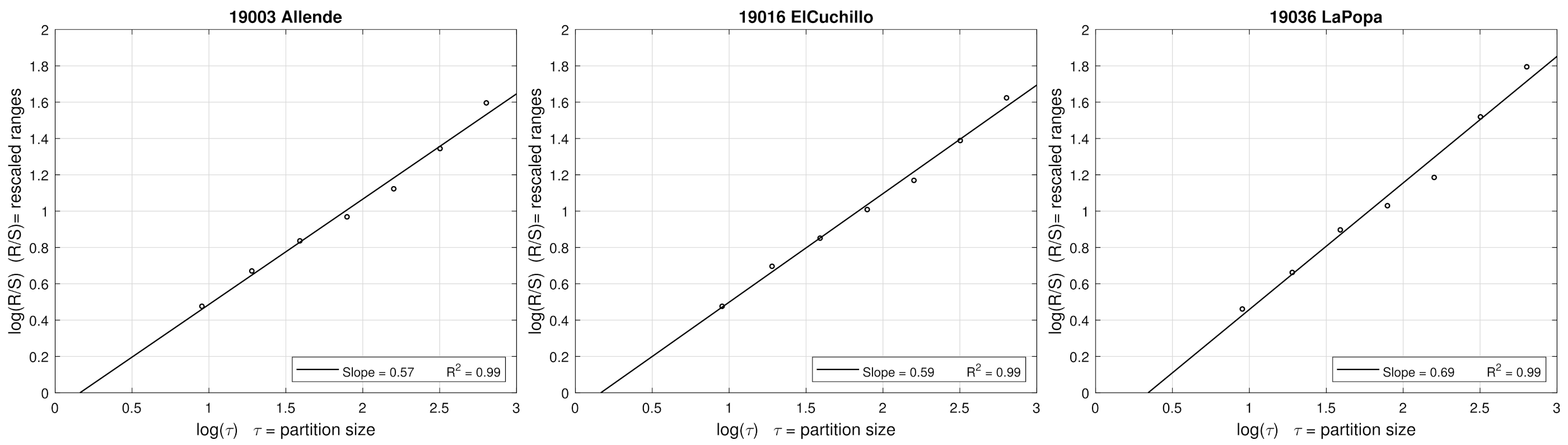
2.1. Hurst Exponent (Hrs)
- 1.
- Calculate the mean and the standard deviation of the subseries.
- 2.
- Determine the variation of each term with respect to the mean:
- 3.
- Obtain the accumulated sum of variation until the ith-term:
- 4.
- Calculate the range of each subseries:
- 5.
- Normalize the calculated ranges (this is why it is called rescaled range):
- 6.
- Once this is done for each subseries of length m, they are averaged:
- 7.
- Finally, the relation of the statistic is given by the following power law:where H refers to Hrs and its a dimensionless number, and is a constant.
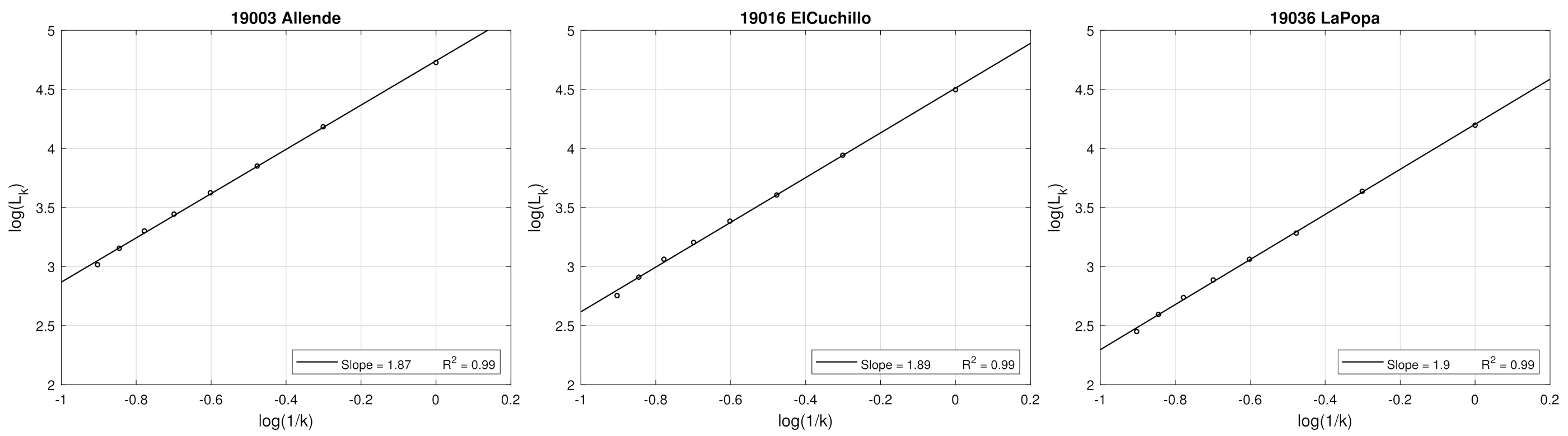
2.2. Higuchi Fractal Dimension (HFD)
3. Results
4. Discussion
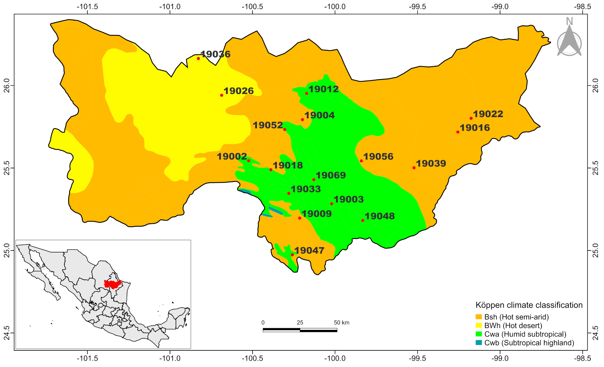
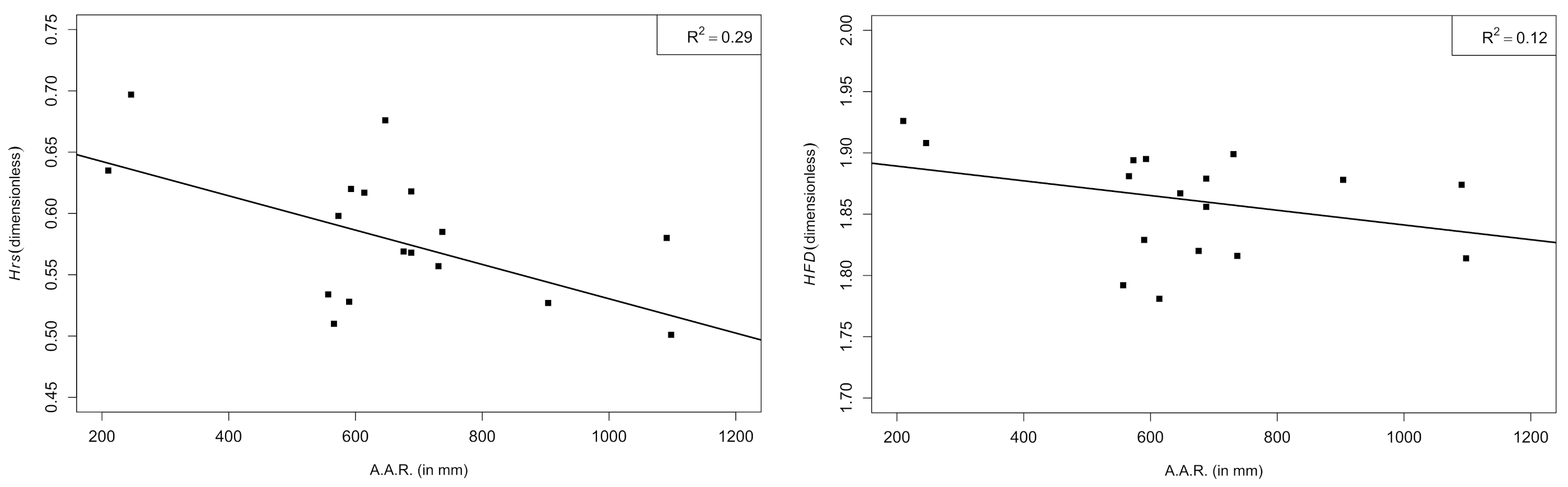
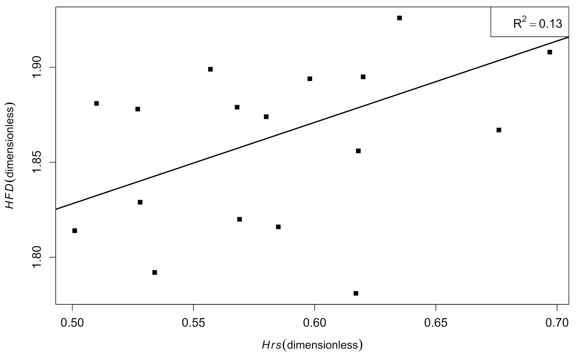
- The RBSJ Basin is a complex region composed by mainly three climates Cwa, Bsh and BWh. Its complexity consists of a geographical mixing of those climates, which makes it difficult to perform a good interpolation by traditional techniques like the Köppen climate classification and A.A.R., and even by more complex techniques like Hrs and HFD. Indeed, about five weather stations are located in the border of zones cataloged as subtropical (Cwa) and semi-arid (Bsh) climates.
- Nevertheless, fractal exponents have shown to have a relation with climates (HFD) and in a weaker sense with A.A.R., which have been reported previously in regions with similar climates [40,41]. In this manner, our study aims to suggest the use of those fractal exponents as an alternative way to understand and complete the climate maps of the region study, positioning HFD as a measure of classification at the same level of A.A.R., and having as an advantage the memory of the time that the method posses.
- As future research, we propose to determine the relation between and the weather to a regional scale, extending this to east and north, where the weather is similar, and considering other regions like Veracruz, Tabasco and Chiapas, which are southeast Mexico’s states where the weather is different to the studied region. In this form, it could be possible to analyze if the correlation between and the weather change lightly or radically. In the first case, the relation will be not a regional case, and it will derive to a larger scale.
5. Conclusions
Author Contributions
Funding
Institutional Review Board Statement
Informed Consent Statement
Data Availability Statement
Acknowledgments
Conflicts of Interest
Appendix A

| Station | Name | 7 | 8 | 9 | 10 | 11 | 12 | |
|---|---|---|---|---|---|---|---|---|
| 19002 | Agua Blanca | 1.72 | 1.75 | 1.78 | 1.81 | 1.86 | 1.90 | 1.95 |
| 19018 | El Pajonal | 1.74 | 1.76 | 1.79 | 1.82 | 1.86 | 1.91 | 1.95 |
| 19069 | La Boca | 1.76 | 1.78 | 1.81 | 1.84 | 1.88 | 1.93 | 1.98 |
| 19033 | Laguna De Sánchez | 1.77 | 1.78 | 1.81 | 1.84 | 1.88 | 1.93 | 1.98 |
| 19047 | Mimbres | 1.76 | 1.78 | 1.82 | 1.85 | 1.88 | 1.91 | 1.95 |
| 19009 | Casillas | 1.78 | 1.80 | 1.82 | 1.86 | 1.89 | 1.93 | 1.98 |
| 19039 | Las Enramadas | 1.81 | 1.83 | 1.85 | 1.87 | 1.91 | 1.94 | 1.99 |
| 19012 | Cienega De Flores | 1.82 | 1.84 | 1.86 | 1.89 | 1.91 | 1.94 | 1.97 |
| 19003 | Allende | 1.83 | 1.85 | 1.87 | 1.89 | 1.91 | 1.94 | 1.99 |
| 19048 | Montemorelos | 1.84 | 1.85 | 1.87 | 1.89 | 1.91 | 1.94 | 1.98 |
| 19052 | Monterrey | 1.84 | 1.85 | 1.87 | 1.89 | 1.91 | 1.95 | 1.99 |
| 19004 | Apodaca | 1.84 | 1.86 | 1.88 | 1.89 | 1.91 | 1.94 | 1.97 |
| 19016 | El Cuchillo | 1.84 | 1.86 | 1.89 | 1.91 | 1.92 | 1.95 | 1.98 |
| 19022 | General Bravo | 1.85 | 1.86 | 1.89 | 1.91 | 1.92 | 1.94 | 1.97 |
| 19056 | San Juan | 1.85 | 1.87 | 1.89 | 1.90 | 1.92 | 1.95 | 1.98 |
| 19036 | La Popa | 1.87 | 1.88 | 1.90 | 1.91 | 1.93 | 1.95 | 1.97 |
| 19026 | Icamole | 1.91 | 1.91 | 1.92 | 1.93 | 1.93 | 1.94 | 1.97 |
References
- Trenberth, K. Changes in Precipitation with Climate Change. Climate Change Research. Clim. Res. 2011, 47, 123–138. [Google Scholar] [CrossRef] [Green Version]
- Trenberth, K. The Impact of Climate Change and Variability on Heavy Precipitation, Floods, and Droughts; John Wiley & Sons, Ltd.: Hoboken, NJ, USA, 2008. [Google Scholar] [CrossRef] [Green Version]
- Zhang, H.; Liu, H.; Zhao, J.; Wang, L.; Li, G.; Huangfu, C.; Wang, H.; Lai, X.; Li, J.; Yang, D. Elevated precipitation modifies the relationship between plant diversity and soil bacterial diversity under nitrogen deposition in Stipa baicalensis steppe. Appl. Soil Ecol. 2017, 119, 345–353. [Google Scholar] [CrossRef]
- Assouline, S.; Mualem, Y. Modeling the dynamics of soil seal formation: Analysis of the effect of soil and rainfall properties. Water Resour. Res. 2000, 36, 2341–2350. [Google Scholar] [CrossRef] [Green Version]
- Tabari, H. Climate change impact on flood and extreme precipitation increases with water availability. Sci. Rep. 2020, 10, 13768. [Google Scholar] [CrossRef]
- Nathan, O.O.; Felix, N.K.; Milka, K.N.; Anne, M.; Noah, A.; Daniel, M.N. Suitability of different data sources in rainfall pattern characterization in the tropical central highlands of Kenya. Heliyon 2020, 6, e05375. [Google Scholar] [CrossRef]
- Potter, N.J.; Chiew, F.H.S.; Charles, S.P.; Fu, G.; Zheng, H.; Zhang, L. Bias in dynamically downscaled rainfall characteristics for hydroclimatic projections. Hydrol. Earth Syst. Sci. 2020, 24, 2963–2979. [Google Scholar] [CrossRef]
- Mandelbrot, B. Statistical Methodology for Nonperiodic Cycles: From the Covariance To R/S Analysis. In Annals of Economic and Social Measurement, Volume 1, Number 3; National Bureau of Economic Research, Inc.: Cambridge, MA, USA, 1972; pp. 259–290. [Google Scholar]
- Hurst, H. A Suggested Statistical Model of some Time Series which occur in Nature. Nature 1957, 180, 494. [Google Scholar] [CrossRef]
- Mandelbrot, B.B.; Wallis, J.R. Robustness of the rescaled range R/S in the measurement of noncyclic long run statistical dependence. Water Resour. Res. 1969, 5, 967–988. [Google Scholar] [CrossRef]
- Breslin, M.; Belward, J. Fractal dimensions for rainfall time series. Math. Comput. Simul. 1999, 48, 437–446. [Google Scholar] [CrossRef]
- Sivakumar, B. Is a chaotic multi-fractal approach for rainfall possible? Hydrol. Process. 2001, 15, 943–955. [Google Scholar] [CrossRef]
- Matsoukas, C.; Islam, S.; Rodriguez-Iturbe, I. Detrended fluctuation analysis of rainfall and streamflow time series. J. Geophys. Res. Atmos. 2000, 105, 29165–29172. [Google Scholar] [CrossRef]
- Olsson, J.; Niemczynowicz, J.; Berndtsson, R. Fractal analysis of high-resolution rainfall time series. J. Geophys. Res. Atmos. 1993, 98, 23265–23274. [Google Scholar] [CrossRef]
- Palanikumar, R.; Sathyamoorthy, D. An alternative approach to characterize time series data: Case study on Malaysian rainfall data. Chaos Solitons Fractals 2006, 27, 511–518. [Google Scholar] [CrossRef]
- Rehman, S.; Siddiqi, A. Wavelet based hurst exponent and fractal dimensional analysis of Saudi climatic dynamics. Chaos Solitons Fractals 2009, 40, 1081–1090. [Google Scholar] [CrossRef]
- Mihailović, D.T.; Nikolić-Đorić, E.; Malinović-Milićević, S.; Singh, V.P.; Mihailović, A.; Stošić, T.; Stošić, B.; Drešković, N. The Choice of an Appropriate Information Dissimilarity Measure for Hierarchical Clustering of River Streamflow Time Series, Based on Calculated Lyapunov Exponent and Kolmogorov Measures. Entropy 2019, 21, 215. [Google Scholar] [CrossRef] [PubMed] [Green Version]
- Chandrasekaran, S.; Poomalai, S.; Balamurali, S.; Sumila, S.; Keerthi, S.; Farveen, A. An Investigation on Relationship between Hurst exponent and Predictability of a Rainfall Time Series. Meteorol. Appl. 2019, 26, 511–519. [Google Scholar] [CrossRef] [Green Version]
- Pal, S.; Dutta, S.; Nasrin, T.; Chattopadhyay, S. Hurst exponent approach through rescaled range analysis to study the time series of summer monsoon rainfall over northeast India. Theor. Appl. Climatol. 2020, 142, 581–587. [Google Scholar] [CrossRef]
- Hurst, H.E. Long-Term Storage Capacity of Reservoirs. Trans. Am. Soc. Civ. Eng. 1951, 116, 770–799. [Google Scholar] [CrossRef]
- Voss, R.F. Random Fractals: Characterization and measurement. In Scaling Phenomena in Disordered Systems; Pynn, R., Skjeltorp, A., Eds.; Springer: Boston, MA, USA, 1991; pp. 1–11. [Google Scholar] [CrossRef]
- Mukherjee, S. Contrasting predictability of summer monsoon rainfall ISOs over the northeastern and western Himalayan region: An application of Hurst exponent. Meteorol. Atmos. Phys. 2019, 131, 55–61. [Google Scholar] [CrossRef]
- Kantelhardt, J.; Koscielny-Bunde, E.; Rybski, D.; Braun, P.; Bunde, A.; Havlin, S. Long-term persistence and multifractality of precipitation and river runoff records. J. Geophys. Res 2006, 111. [Google Scholar] [CrossRef]
- López-Lambraño, A.A.; Fuentes, C.; López-Ramos, A.A.; Mata-Ramírez, J.; López-Lambraño, M. Spatial and temporal Hurst exponent variability of rainfall series based on the climatological distribution in a semiarid region in Mexico. Atmósfera 2018, 31, 199–219. [Google Scholar] [CrossRef]
- Sun, J.; Wang, X.; Shahid, S. Precipitation and runoff variation characteristics in typical regions of North China Plain: A case study of Hengshui City. Theor. Appl. Climatol. 2020, 142, 971–985. [Google Scholar] [CrossRef]
- Anis, A.A.; Lloyd, E.H. The Expected Value of the Adjusted Rescaled Hurst Range of Independent Normal Summands. Biometrika 1976, 63, 111–116. [Google Scholar] [CrossRef]
- Kalauzi, A.; Čukić, M.; Millán, H.; Bonafoni, S.; Biondi, R. Comparison of fractal dimension oscillations and trends of rainfall data from Pastaza Province, Ecuador and Veneto, Italy. Atmos. Res. 2009, 93, 673–679. [Google Scholar] [CrossRef]
- Ciobotaru, A.M.; Andronache, I.; Dey, N.; Petralli, M.; Mansouri Daneshvar, M.R.; Wang, Q.; Radulovic, M.; Pintilii, R. Temperature-Humidity Index described by fractal Higuchi Dimension affects tourism activity in the urban environment of Focşani City (Romania). Theor. Appl. Climatol. 2019, 136, 1009–1019. [Google Scholar] [CrossRef]
- Sanchez-Castillo, L.; Kubota, T.; Silva, I.C. Critical Rainfall for the Triggering of Sediment Related Disasters under the Urban Forest Development in Nuevo Leon, Mexico. Int. J. Ecol. Dev. 2015, 30, 1–10. [Google Scholar]
- Návar Cháidez, J. Water Scarcity and Degradation in the Rio San Juan Watershed of Northeastern Mexico. Front. Norte 2011, 46, 125–150. [Google Scholar]
- García, E. Comisión Nacional para el Conocimiento y Uso de la Biodiversidad (CONABIO). Climas (Clasificación de Koppen). 1998. Available online: http://www.conabio.gob.mx/informacion/gis/ (accessed on 1 September 2021).
- Benavides-Bravo, F.G.; Soto-Villalobos, R.; Cantú-González, J.R.; Aguirre-López, M.A.; Benavides-Ríos, A.G. A Quadratic–Exponential Model of Variogram Based on Knowing the Maximal Variability: Application to a Rainfall Time Series. Mathematics 2021, 9, 2466. [Google Scholar] [CrossRef]
- Villanueva-Hernández, H.; Tovar-Cabañas, R.; Vargas-Castilleja, R. Classification of aquifers in the Mina field, Nuevo Leon, using geographic information systems. Tecnol. Cienc. Agua 2014, 10, 96–123. [Google Scholar] [CrossRef]
- Benítez-García, S.E.; Kanda, I.; Wakamatsu, S.; Okazaki, Y.; Kawano, M. Analysis of Criteria Air Pollutant Trends in Three Mexican Metropolitan Areas. Atmosphere 2014, 5, 806–829. [Google Scholar] [CrossRef] [Green Version]
- Köppen, W. Klassifikation der Klimate nach Temperatur, Niederschlag und Jahreslauf (Classification of climates according to temperature, precipitation and seasonal cycle). Petermanns Geogr. Mitteilungen 1918, 64, 193–203, 243–248. [Google Scholar]
- Bassingthwaighte, J.B.; Raymond, G.M. Evaluating rescaled range analysis for time series. Ann. Biomed. Eng. 1994, 22, 432–444. [Google Scholar] [CrossRef]
- Benavides-Bravo, F.; Almaguer, F.; Soto-Villalobos, R.; Tercero-Gómez, V.; Morales-Castillo, J. Clustering of Rainfall Stations in RH-24 Mexico Region Using the Hurst Exponent in Semivariograms. Math. Probl. Eng. 2015, 2015, 629254. [Google Scholar] [CrossRef] [Green Version]
- Higuchi, T. Approach to an irregular time series on the basis of the fractal theory. Phys. D Nonlinear Phenom. 1988, 31, 277–283. [Google Scholar] [CrossRef]
- Bashan, A.; Bartsch, R.; Kantelhardt, J.W.; Havlin, S. Comparison of detrending methods for fluctuation analysis. Phys. A Stat. Mech. Its Appl. 2008, 387, 5080–5090. [Google Scholar] [CrossRef] [Green Version]
- Nicholson, S.E. Revised Rainfall Series for the West African Subtropics. Mon. Weather Rev. 1979, 107, 620–623. [Google Scholar] [CrossRef] [Green Version]
- Valle, M.A.V.; García, G.M.; Cohen, I.S.; Oleschko, L.K.; Corral, J.A.R.; Korvin, G. Spatial Variability of the Hurst Exponent for the Daily Scale Rainfall Series in the State of Zacatecas, Mexico. J. Appl. Meteorol. Climatol. 2013, 52, 2771–2780. [Google Scholar] [CrossRef]


| Station | Name | Latitude | Longitude | Hrs | HFD | A.A.R. | Climate |
|---|---|---|---|---|---|---|---|
| 19002 | Agua Blanca | 25.5442 | −100.5231 | 0.62 | 1.78 | 614 | Cwa |
| 19018 | El Pajonal | 25.4897 | −100.3889 | 0.50 | 1.79 | 557 | Cwa |
| 19069 | La Boca | 25.4294 | −100.1289 | 0.48 | 1.81 | 1098 | Cwa |
| 19033 | Laguna de Sánchez | 25.3461 | −100.2800 | 0.57 | 1.81 | 737 | Cwa |
| 19047 | Mimbres | 24.9739 | −100.2586 | 0.54 | 1.82 | 676 | Cwa |
| 19009 | Casillas | 25.1964 | −100.2142 | 0.48 | 1.82 | 590 | Bsh |
| 19039 | Las Enramadas | 25.5014 | −99.5214 | 0.62 | 1.85 | 688 | Bsh |
| 19012 | Ciénega de Flores | 25.9522 | −100.1722 | 0.70 | 1.86 | 647 | Cwa |
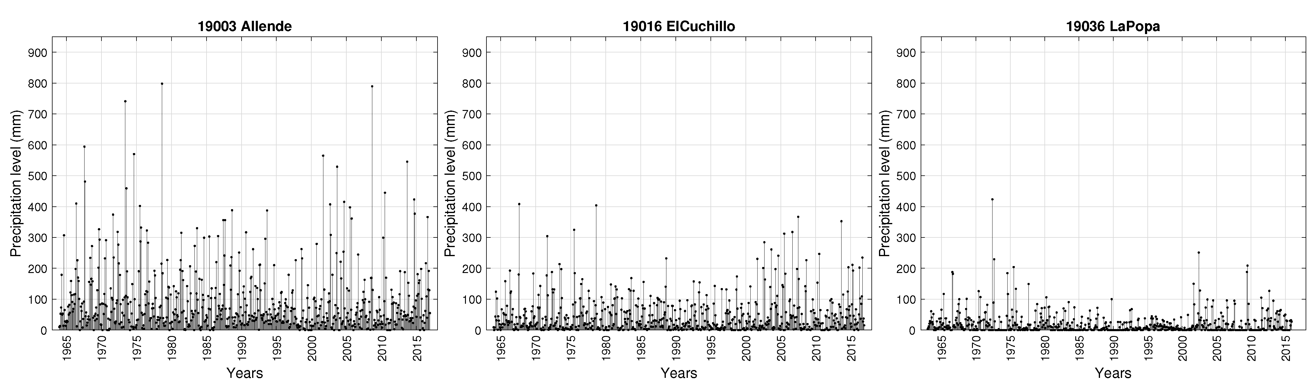
| 19003 | Allende | 25.2836 | −100.0203 | 0.57 | 1.87 | 1091 | Cwa |
| 19048 | Montemorelos | 25.1819 | −99.8322 | 0.50 | 1.87 | 904 | Cwa |
| 19052 | Monterrey | 25.7336 | −100.3047 | 0.56 | 1.87 | 688 | Cwa |
| 19004 | Apodaca | 25.7936 | −100.1972 | 0.48 | 1.88 | 566 | Bsh |
| 19016 | El Cuchillo | 25.7181 | −99.2558 | 0.58 | 1.89 | 573 | Bsh |
| 19022 | General Bravo | 25.8014 | −99.1756 | 0.62 | 1.89 | 593 | Bsh |
| 19056 | San Juan | 25.5433 | −99.8403 | 0.53 | 1.89 | 731 | Bsh |
| 19036 | La Popa | 26.1639 | −100.8278 | 0.71 | 1.90 | 246 | BWh |
| 19026 | Icamole | 25.9411 | −100.6869 | 0.63 | 1.92 | 210 | BWh |
Publisher’s Note: MDPI stays neutral with regard to jurisdictional claims in published maps and institutional affiliations. |
© 2021 by the authors. Licensee MDPI, Basel, Switzerland. This article is an open access article distributed under the terms and conditions of the Creative Commons Attribution (CC BY) license (https://creativecommons.org/licenses/by/4.0/).
Share and Cite
Benavides-Bravo, F.G.; Martinez-Peon, D.; Benavides-Ríos, Á.G.; Walle-García, O.; Soto-Villalobos, R.; Aguirre-López, M.A. A Climate-Mathematical Clustering of Rainfall Stations in the Río Bravo-San Juan Basin (Mexico) by Using the Higuchi Fractal Dimension and the Hurst Exponent. Mathematics 2021, 9, 2656. https://doi.org/10.3390/math9212656
Benavides-Bravo FG, Martinez-Peon D, Benavides-Ríos ÁG, Walle-García O, Soto-Villalobos R, Aguirre-López MA. A Climate-Mathematical Clustering of Rainfall Stations in the Río Bravo-San Juan Basin (Mexico) by Using the Higuchi Fractal Dimension and the Hurst Exponent. Mathematics. 2021; 9(21):2656. https://doi.org/10.3390/math9212656
Chicago/Turabian StyleBenavides-Bravo, Francisco Gerardo, Dulce Martinez-Peon, Ángela Gabriela Benavides-Ríos, Otoniel Walle-García, Roberto Soto-Villalobos, and Mario A. Aguirre-López. 2021. "A Climate-Mathematical Clustering of Rainfall Stations in the Río Bravo-San Juan Basin (Mexico) by Using the Higuchi Fractal Dimension and the Hurst Exponent" Mathematics 9, no. 21: 2656. https://doi.org/10.3390/math9212656