Article

An Information-Theoretic Approach for Multivariate Skew-t Distributions and Applications †

by
Salah H. Abid
1,
Uday J. Quaez
1 and
Javier E. Contreras-Reyes
2,*
1
Department of Mathematics, Education College, Al-Mustansiriya University, Baghdad 14022, Iraq
2
Instituto de Estadística, Facultad de Ciencias, Universidad de Valparaíso, Valparaíso 2360102, Chile
*
Author to whom correspondence should be addressed.
This work corresponds to a revised, corrected and extended version of the pre-print: Abid, S.H., Quaez, U.J. (2019). Renyi and Shannon Entropies of Finite Mixtures of Multivariate Skew t-distributions. arXiv:1901.10569.
Mathematics 2021, 9(2), 146; https://doi.org/10.3390/math9020146
Submission received: 17 December 2020 / Revised: 6 January 2021 / Accepted: 8 January 2021 / Published: 11 January 2021
(This article belongs to the Special Issue Probability, Statistics and Their Applications)

Abstract

:
Shannon and Rényi entropies are two important measures of uncertainty for data analysis. These entropies have been studied for multivariate Student-t and skew-normal distributions. In this paper, we extend the Rényi entropy to multivariate skew-t and finite mixture of multivariate skew-t (FMST) distributions. This class of flexible distributions allows handling asymmetry and tail weight behavior simultaneously. We find upper and lower bounds of Rényi entropy for these families. Numerical simulations illustrate the results for several scenarios: symmetry/asymmetry and light/heavy-tails. Finally, we present applications of our findings to a swordfish length-weight dataset to illustrate the behavior of entropies of the FMST distribution. Comparisons with the counterparts—the finite mixture of multivariate skew-normal and normal distributions—are also presented.

1. Introduction

Finite mixture models have used in the analysis of heterogeneous datasets due to its flexibility [1]. These models provide important applications in many scientific fields such as density estimation [2], data mining and pattern recognition [3], image processing and satellite imaging [4], medicine and genetics [4,5], fisheries [6,7], astronomy [2], and more. Specifically, Carreira-Perpiñán [2] considered the mixture of normal densities to find the modes of multi-dimensional data via the Shannon entropy. Because no analytical expressions exist for Shannon entropy of normal mixture of densities, the authors of [2] considered bounds to approximates the Shannon entropy [8]. Given that these applications have been developed in the normal mixture of densities context, several calculations of Shannon and Rényi entropies for non-normal distributions exist.
Azzalini and Dalla-Valle [9] and Azzalini and Capitanio [10] introduced the multivariate skew-normal and skew-t distributions as an alternative to multivariate normal distribution to deal with skewness and heavy-tailness in the data, respectively. Lin et al. [11] proposed a development of finite mixture of skew-t (FMST) distributions, and more recently [4] provided an overview of developments of FMST distributions. Arellano-Valle et al. [12] and Contreras-Reyes [13] presented the mutual information and Shannon entropy for multivariate skew-normal and skew-t distributions, respectively. They highlighted that the calculation of mutual information index and Shannon entropy include the negentropy concept represented by a one-dimensional integral. Contreras-Reyes [14] discussed the values of Rényi entropy of multivariate skew-normal and extended skew-normal distributions. Contreras-Reyes and Cortés [6] considered bounds to approximate the Rényi entropy for finite mixture of multivariate skew-normal (FMSN) distributions by using lower and upper bounds. More recently, the authors of [15,16] presented the bounds of Rényi entropy of multivariate skew-normal-Cauchy and skew-Laplace distributions, and [17] considered the Kullback–Leibler divergence based on multivariate skew-t densities [13] as a classifier for an SAR image system.
In this paper, we propose an information-theoretic approach for FMST distributions. The explicit expressions of Shannon and Rényi entropies of skew-t distribution are derived. We give bounds for Rényi entropies of FMST models. An approximate value of these entropies can be calculated. Simulation studies illustrate the behavior of Rényi entropy approximations for a given order α , skewness, and freedom degrees of the proposed mixture model. Numerical simulations illustrates the results for several scenarios: symmetry/asymmetry and light/heavy-tails. Finally, a real data application of a swordfish length-weight dataset is revisited from the work in [6], where the skew-normal model is compared with the proposed skew-t one.
The paper is organized as follows. Section 2 gives the propositions, lemmas, and numerical simulations for computation of Shannon and Rényi entropies of multivariate skew-t random variables. Section 3 provides bounds to approximate Shannon and Rényi entropies for FMST distributions and a numerical application of swordfish data. Finally, Section 4 concludes the study.

2. Multivariate Skew- t Distribution

The multivariate t-distribution corresponds to a generalization of the Student-t-distribution. Let x R d be a random vector, d Z + , is multivariate t-distributed [18], denoted as X T d ( ξ , Ω , ν ) , whose probability density function (pdf) is given by
t d ( x ; ξ , Ω , ν ) = B d ( ν ) | Ω | 1 / 2 1 + Q ( x ) ν ,
where Q ( x ) = ( x ξ ) Ω 1 ( x ξ ) , μ R d is a location parameter, Ω R d × d is a dispersion matrix, ν R is the degree of freedom parameter,
B ( ν ) = Γ ν + 2 Γ ν 2 ( ν π ) / 2 , ν > 0 , Z ,
and Γ ( · ) is the gamma function.
The multivariate normal distribution is obtained from the limit T d ( ξ , Ω , ν ) N d ( ξ , Ω ) , as ν . In the special case where ν = 1 , ξ = 0 and Ω = I d , t d ( ξ , Ω , ν ) leads to the multivariate Cauchy distribution. The mean and variance of random vector x are
E [ X ] = ξ , ν > 1 ,
V [ X ] = B 2 ( ν ) 2 π Ω , ν > 2 ,
respectively.
An extension of multivariate skew-normal distribution is the skew-t one by incorporating a degree of freedom parameter representing the presence of atypical observations in empirical data [10,12,19]. We considered the definition of skew-t distribution given in [12]. Let y R d be a multivariate skew-t random variable with location vector ξ R d , dispersion matrix Ω R d × d , asymmetry vector η R d , and ν > 0 degrees of freedom. We denoted y by Y S T d ( ξ , Ω , η , ν ) if has pdf given by
f ( y ; ξ , Ω , η , ν ) = 2 t d ( y ; ξ , Ω , ν ) T η ¯ Ω 1 / 2 ( y ξ ) ν + d ν + Q ( y ) ; ν + d ,
where η ¯ = Ω 1 / 2 η and T ( x ; ν + d ) T 1 ( x ; 0 , 1 , ν + d ) is the univariate Student-t cumulative distribution function (cdf) of x .
The multivariate Student-t distribution is a special case of the multivariate skew-t one and is related to a multivariate skew-normal random variable through equation
Y = d ξ + V 1 / 2 Z 0 ,
where Z 0 = Ω 1 / 2 ( Y ξ ) S N d ( 0 , I d , η ) and V χ 2 / ν , and they are independent, where S N d and χ 2 denotes the d-variate skew-normal [9] and univariate chi-square distribution [10], respectively. The multivariate skew-t distribution yields the multivariate skew-normal and Student-t ones as ν and when η = 0 , respectively [4].
Considering the m-cumulant function
E ( V m / 2 ) = B m ( ν ) ( 2 π ) m / 2 , m 1 , ν > m ,
and Equations (2)–(4), the mean vector and covariance matrix of Y are, respectively, derived by the authors of [10] in the following forms,
E [ Y ] = ξ + B 1 ( ν ) π η ¯ , ν > 1 ,
V [ Y ] = ξ ξ + B 2 ( ν ) 2 π Ω + B 1 ( ν ) π 2 ( ξ δ + δ ξ ) , ν > 2 ,
where δ = Ω η / 1 + η Ω η .

2.1. Entropies

Shannon [20] proposed an entropy to quantify the uncertainty of a system and posteriorly, Rényi [21] generalized the Shannon entropy for any probability distribution related to a discrete or continuous random variable. In this section, we derive these measures for the skew-t case.
Consider a pdf f associated with a random variable y R d , denoted by H ( Y ) , the well-known Shannon entropy [22]. It is defined by
H ( Z ) = R d f ( y ) log f ( y ) d y .
Proposition 1.
The Shannon entropy of Y S T d ( ξ , Ω , η , ν ) is
H ( Y ) = H ( X ) E log 2 T ν + d η ¯ W H ν + d 1 + W H 2 ; ν + k ,
where W H S T 1 ( 0 , 1 , η ¯ , ν + d 1 ) , η ¯ = η ¯ η ¯ = ( η Ω η ) 1 / 2 , and H ( X ) is the Student-t Shannon entropy of X T d ( ξ , Ω , ν ) given by
H ( X ) = 1 2 log | Ω | log B d ( ν ) + Ψ d ( ν ) ,
where
Ψ d ( ν ) = ν + d 2 ψ ν + d 2 ψ ν 2 ,
B d ( ν ) is defined in (2) and ψ ( x ) = d d x log Γ ( x ) is the digamma function.
The proof for the Shannon entropy of Y in (10) is shown in [12]. The same entropy, but for X in (11), was first presented in [23].
An extension of Shannon entropy is the α th Rényi order given by [21]. The Rényi entropy of Y is denoted by R α ( Y ) and defined by
R α ( Y ) = 1 1 α log R d [ f ( y ) ] α d y ,
with 0 < α < , α 1 , and where normalization to unity as given by R d f ( y ) d y = 1  [24]. The Shannon entropy is obtained from R α ( Y ) as α 1 [14,21]. The Rényi entropy is invariant under a location transformation, but not invariant under a scale transformation. For any α 1 < α 2 , we have R α 1 ( Y ) R α 2 ( Y ) , and R α 1 ( Y ) = R α 2 ( Y ) if and only if the system is uniformly distributed.
In order to compute the Rényi entropy of a multivariate skew-t random variate, we need the following preliminary results that involve the pdf (5).
Lemma 1.
Let Y S T d ( ξ , Ω , η , ν ) . Then,
E log 2 T η ¯ Ω 1 / 2 ( y ξ ) ν + d ν + Q ( y ) ; ν + d = E log 2 T ν + d η ¯ X 0 ν + d 1 + X 0 2 ; ν + d 2 T ν + 1 η ¯ X 0 ν + X 0 2 ; ν + d ,
where X 0 T 1 ( 0 , 1 , ν + d 1 ) .
Proof. 
We directly get
E log 2 T η ¯ Ω 1 / 2 ( Y ξ ) ν + d ν + Q ( Y ) ; ν + d = R d log 2 T η ¯ Ω 1 / 2 ( y ξ ) ν + d ν + Q ( y ) ; ν + d × 2 t d ( y ; ξ , Ω , ν ) T η ¯ Ω 1 / 2 ( y ξ ) ν + d ν + Q ( y ) ; ν + d d y .
Using the change of variables z 0 = Ω 1 / 2 ( y ξ ) , we get that Z 0 S T d ( 0 , I d , η , ν ) and the determinant of Jacobian matrix | Ω | 1 / 2 . Therefore,
E log 2 T η ¯ Ω 1 / 2 ( Y ξ ) ν + d ν + Q ( Y ) ; ν + d = R d log 2 T η ¯ z 0 ν + d ν + z 0 z 0 ; ν + d × 2 | Ω | 1 / 2 t d ( z 0 ; 0 , I d , ν ) T η ¯ z 0 ν + d ν + z 0 z 0 ; ν + d d y = E log 2 T η ¯ Z 0 ν + d ν + Z 0 Z 0 ; ν + d .
Lemma 3 of [12] implies that
E log 2 T η ¯ Ω 1 / 2 ( Y ξ ) ν + d ν + Q ( Y ) ; ν + d = E log 2 T ν + d η ¯ W R ν + d 1 + W R 2 ; ν + d ,
with W R S T 1 ( 0 , 1 , η ¯ , ν + d 1 ) and η ¯ = η ¯ η ¯ . The latter result yields the proof.    □
Lemma 1 allows us to compute an expected value of a d-variate random variable Y as an expected value of a univariate Student-t one X 0 . This result is also applied in the computation of Shannon entropy of Y ; however, the latter depends on a univariate skew-t. Then, we can represent the expected value of (10) with respect to a univariate Student-t random variable as follows,
Proposition 2.
Let X T d ( ξ , Ω , ν ) and Y S T d ( ξ , Ω , η , ν ) , the Shannon entropy of Y can be written as
H ( Y ) = H ( X ) N ( X 0 ) ,
where
N ( X 0 ) = E log 2 T ν + d η ¯ X 0 ν + d 1 + X 0 2 ; ν + d 2 T ν + 1 η ¯ X 0 ν + X 0 2 ; ν + d ,
and X 0 T 1 ( 0 , 1 , ν + d 1 ) .
Proof. 
By computing the natural logarithm and expectation in both sides of pdf (5), we have
E log { f ( Y ; ξ , Ω , η , ν ) } = E [ log { t d ( Y ; ξ , Ω , ν ) } ] + E log 2 T η ¯ Ω 1 / 2 ( Y ξ ) ν + d ν + Q ( Y ) ; ν + d .
Using Lemma 1 and Proposition 1 of [25], we obtain
H ( Y ) = H ( X ) E log 2 T η ¯ Ω 1 / 2 ( Y ξ ) ν + d ν + Q ( Y ) ; ν + d .
Then, Lemma 1 gives us the required result for this proof.    □
Lemma 1 and Proposition 2 decompose the expected value into two parts; however, it is still necessary to solve the integral (13) that involves parameter α . The next Lemma uses the previous results to obtain the skew-t Rényi entropy.
Lemma 2.
Let Y S T d ( ξ , Ω , η , ν ) . Then,
R d [ f ( y ; ξ , Ω , η , ν ) ] α d y = C α , d ( Ω , ν ) E 2 T ν + d η ¯ X 0 ν + d 1 + X 0 2 ; ν + d α ,
where
C α , d ( Ω , ν ) = | Ω | α / 2 [ B d ( ν ) ] α B d ( α [ ν + d ] ) ν α [ ν + d ] d / 2 ,
and X 0 T 1 ( 0 , 1 , β ) , β = α ( ν + d ) d , 0 < α < , α 1 .
Proof. 
Using the change of variables z 0 = Ω 1 / 2 ( y ξ ) associated with Jacobian matrix determinant | Ω | 1 / 2 in Equation (5), we get
R d [ f ( y ; ξ , Ω , η , ν ) ] α d y = B d ( ν ) | Ω | 1 / 2 α R d 1 + z 0 z 0 ν α ( ν + d 2 ) 2 T η ¯ z 0 ν + d ν + z 0 z 0 ; ν + d α d z 0 .
By replacing β = α ( ν + d ) d and using the change of variables u = z 0 β ν , we obtain
R d [ f ( y ; ξ , Ω , η , ν ) ] α d y = B d ( ν ) | Ω | 1 / 2 α ν β d 2 R d 1 + u u β α ( u + d 2 ) 2 T η ¯ u ν + d β + u u ; ν + d α d u = B d ( ν ) | Ω | 1 / 2 α ν β d 2 1 B d ( ν ) E 2 T η ¯ U ν + d β + U U ; ν + d α ,
where U T d ( 0 , I d , β ) . The proof is completed by using Lemma 3 of [12].   □
By taking natural logarithm and multiplying by ( 1 α ) 1 in both sides of Equation (15), the Lemma 2 yields the final expression of skew-t Rényi entropy as is presented in the next Proposition.
Proposition 3.
The Rényi entropy of Y S T d ( ξ , Ω , η , ν ) is
R α ( Y ) = R α ( X ) + 1 1 α log E 2 T ν + d η ¯ W R α ( ν + d ) 1 + W R 2 ; ν + d α ,
where R α ( X ) is the Student-t Rényi entropy of X T d ( ξ , Ω , ν ) given by
R α ( X ) = H ( X ) + 1 1 α log C α , d ( Ω , ν ) ,
H ( X ) is the Student-t Shannon entropy of X given in (11), W R T 1 ( 0 , 1 , β ) , β = α ( ν + d ) d , and C α , d ( Ω , ν ) is given in Lemma 2.
It is easy to observe that skew-t Shannon entropy is obtained from (16) by taking the limit as α converges to 1.

2.2. Computational Implementation and Numerical Simulations
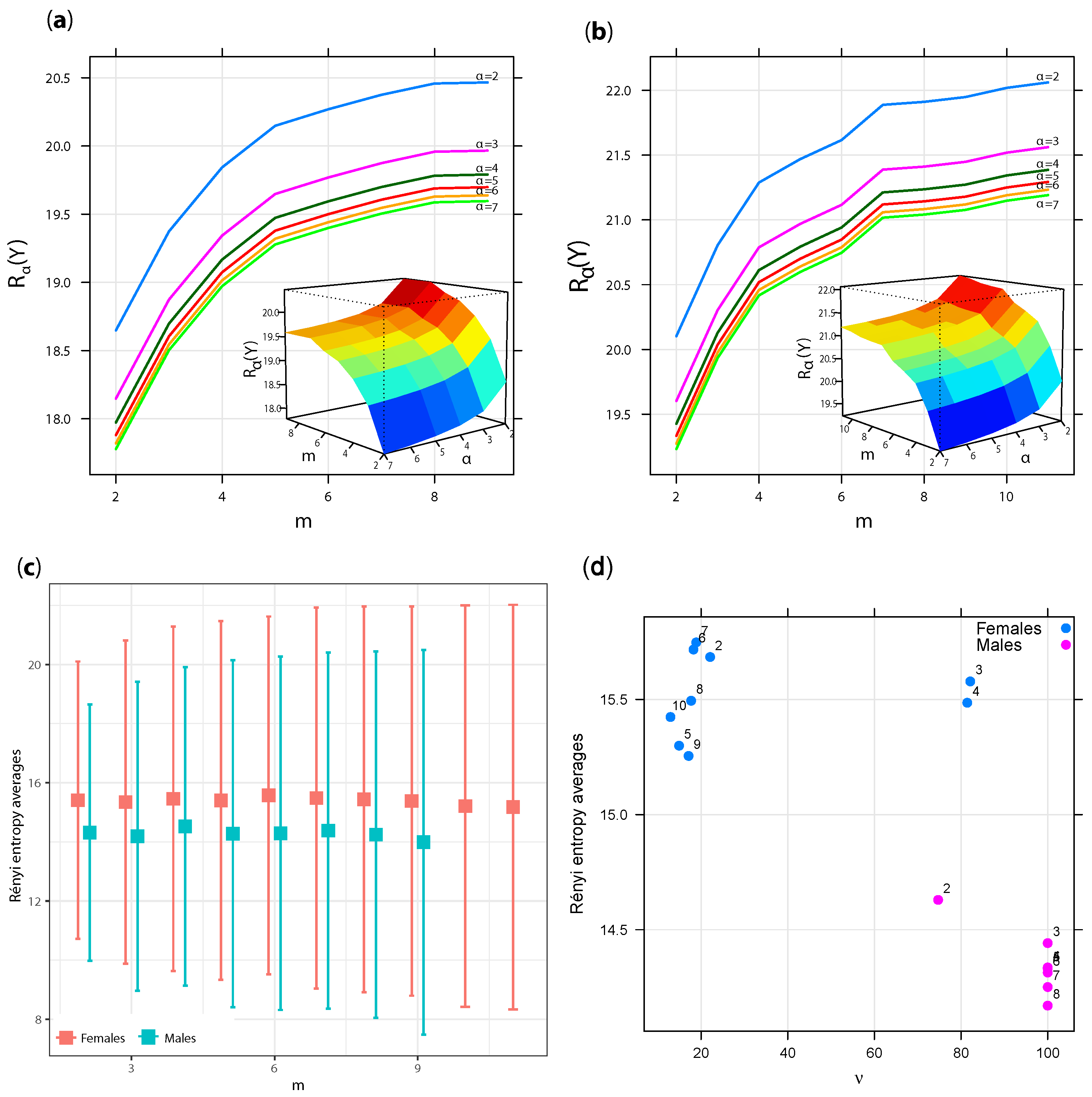
All numerical computations were made with R software [26]. The integrals of skew-t Rényi entropies of Equation (16) were evaluated using the integrate function of R software’s QUADPACK routine [27]. This method allows to integrate the Student-t cdf of Equation (16) in the interval ( , ) . This section illustrates the relationship between parameters α , η , and ν with Rényi entropy for d = 1 , 2, 3, and 4 dimensions. Consider Y S T d ( ξ , Ω , η , ν ) with the following cases.
(a) 
d = 1 , ξ = 0 , Ω = 1.5 , and η = 0.3 .
(b) 
d = 2 , ξ = 0 , Ω = 0.7 0.3 0.3 3 , and η = 0.3 2 .
(c) 
d = 3 , ξ = 0 , Ω = I 3 , and η = 0.3 2 0.3 .
(d) 
d = 4 , ξ = 0 , Ω = I 4 , and η = 0.3 2 0.3 0.5 .
Figure 1 shows the relationship between Rényi entropy of Y and ν = 3 , , 30 , α = 2 , 3 , 4 , 5 , 6 , 8 , 10 , and d = 1 , 2 , 3 , 4 , related to cases (a)–(d). The Rényi entropies converge to a finite value for all α and ν , and increase for increments of d. The dispersion matrix Ω plays an important role in Rényi entropy, mainly by the increment of matrix dimension related to d. Moreover, the Rényi entropy decreases when α increases, as mentioned in the properties of R α ( Y ) . The Rényi entropies decrease when ν increases, yielding the respective Student-t Rényi entropies ( ν ).
Subplot of case (a) considered negative and positive values of η ( 6 η 6 ), producing a symmetry of R α ( Y ) with respect to this parameter. However, as mentioned below, R α ( Y ) decreases for increments of ν . Subplots of cases (b)–(d) cannot represent the behavior of η given this parameter’s dimension d = 2 , 3 , 4 of. For these cases, order α is considered and the Rényi entropy decreases when α increases.

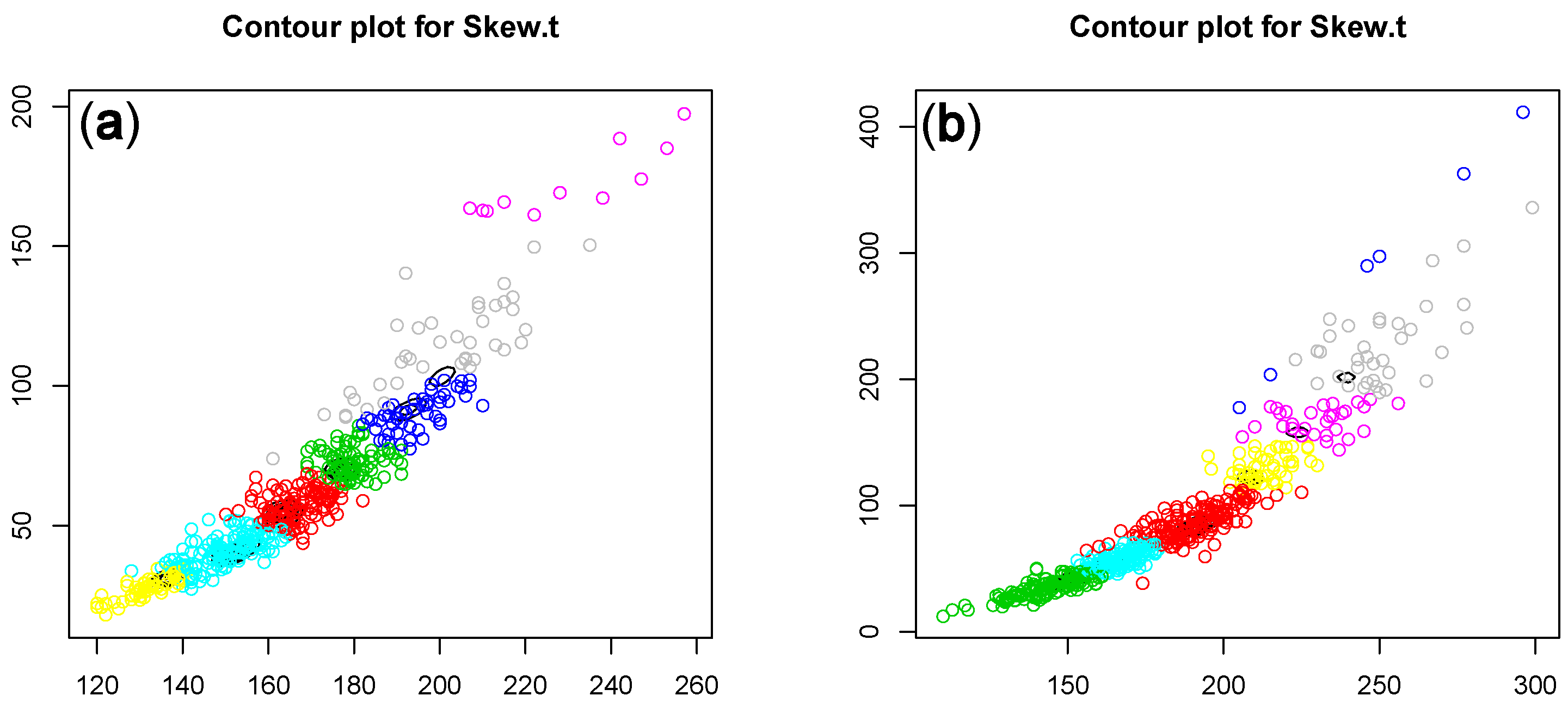
3. Application to Finite Mixtures of Multivariate Skew- t Distributions

Let us consider the definitions of [5,7,28] for FMST distributions. The pdf of an m-component mixture model with parameter vector set θ ˜ = ( ξ ˜ , Ω ˜ , Λ ˜ , ν ˜ ) : ξ ˜ = ( ξ 1 , , ξ m ) , a set of m location vector parameters Ω ˜ = ( Ω 1 , , Ω m ) , a set of m dispersion matrices Λ ˜ = ( η 1 , , η m ) , a set of shape vector parameters ν ˜ = ( ν 1 , , ν m ) , a set of degree-of-freedom parameters, and with m mixing weights p = ( p 1 , , p m ) is
p ( y ˜ ; θ ˜ , π ) = j = 1 m p j f ( y j ; θ j ) ,
where p j 0 , j = 1 m p j = 1 , y ˜ = ( y 1 , , y m ) , and f ( y j ; θ j ) are defined as in (5) for a known θ j = ( ξ j , Ω j , η j , ν j ) , j = 1 , , m . If Y ˜ has pdf (18), it is denoted as Y ˜ F M S T d ( θ ˜ , p ) .
Let S i = ( S i , 1 , , S i , m ) with j = 1 m S i j = 1 be a set of m latent indicators of observations y ˜ , i = 1 , , n , where j corresponds to a binary index such that S i j = 1 , if Y i is from group j, and S i j = 0 otherwise. Then, indicators S 1 , , S n are independent and each one with multinomial distribution given by
p ( s i ) = p 1 s i , 1 p 2 s i , 2 1 j = 1 m 1 p j s i , m
and denoted as S i M ( 1 ; p 1 , , p m ) . Proposition 1 of the work in [28] and (6) allow obtaining a hierarchical representation to each j-th component pdf (see Section 3.1 of [28] for details). This hierarchical representation is useful for parameter estimation based on EM framework for FMST distributions.
The first and second moments of the j-th component Y j , (7) and (8), respectively, get the first two moments of Y ˜ :
E [ Y ˜ ] = j = 1 m p j ξ j + B 1 ( ν ) π η ¯ j ,
V [ Y ˜ ] = j = 1 m p j ξ j ξ j + B 2 ( ν ) 2 π Ω j + B 1 ( ν ) π 2 ( ξ j δ j + δ j ξ j ) + μ j μ j ,
where
μ j = ξ j + B 1 ( ν ) π η ¯ j E [ Y ˜ ] ,
η ¯ j = Ω j 1 / 2 η j , and
δ j = Ω j η j 1 + η j Ω j η j , j = 1 , , m ;
see, e.g., in [2,6].
Dehesa et al. [24] obtained an upper bound of Rényi entropy using a variational approach that expresses the Rényi entropy of a finite mixture random variable in terms of the dispersion matrix. Specifically, the result provided by [29] allows obtaining a lower bound for Rényi entropy of an FMST in terms of each component (see also [6]), as is presented next.
log [ E α ( Y ˜ ) ] 1 α R α ( Y ˜ ) d 2 log V [ Y ˜ ] d + F α ( d ) ,
with
E α ( Y ˜ ) = e ( 1 α ) R α ( Y m ) + j = 1 m 1 k = 1 j p k α e ( 1 α ) R α ( Y j ) e ( 1 α ) R α ( Y j + 1 )
and
F α ( d ) = log π ( α ( 2 + d ) d ) α 1 + 2 d ( α 1 ) log α ( 2 + d ) d 2 α + 2 d log Γ α α 1 Γ α ( 2 + d ) d 2 ( α 1 ) , if   α > 1 , log π ( α ( 2 + d ) d ) 1 α + 2 α d ( α 1 ) log α ( 2 + d ) d 2 α + 2 d log Γ α ( 2 + d ) d 2 ( 1 α ) Γ α 1 α , if   d d + 2 α 1 , log ( 2 π e ) , if   α = 1 .
On the left side of the inequality (21), the lower bound depends on Rényi entropy of each mixture component. A proof of this lower bound is available in Lemma 1 of [6], obtained from Proposition 1 (B1) of [29]. We can see that the right side of the inequality (21) depends on the dispersion matrix, the shape parameters, the α th order and dimension d. A proof of this upper bound is available in Section 3 of [24]. For the case α = 1 , F α ( d ) is related to Shannon entropy of a multivariate standardized normal random variable.

Swordfish Data Analysis

We considered the dataset used in [6], which corresponds to a sample of 486 and 507 length-weight observations of swordfish males and females, respectively. The swordfish data were sampled in the south Pacific off northern Chile during 2011. The observations were obtained using the sampling program of the Instituto de Fomento Pesquero (IFOP, http://www.ifop.cl/). The dataset includes swordfish from 120 to 257 cm and 110 to 299 cm for males and females, respectively.
Following [6], the length-weight nonlinear function w ( l ) = a l b is considered to explain the increments in swordfish weight w ( l ) in terms of l, where a and b are the theoretical weight at l = 0 and weight growth rate, respectively [30]. The authors obtained a good fitting of w ( l ) after considering a log-transformed w ( l ) . Then, a two-column matrix formed by these variables is obtained for the clustering procedure. This means no collinearity problem exists, given the nonlinear relationship of length and weight variables. Therefore, the length-weight data are evaluated with the FMST model for m = 1 , , m * (where m * is the maximum age by gender) and d = 2 . The FMST parameter estimates were computed using the mixsmsn R software’s library [31].
Figure 2a,b shows the upper bounds for Rényi entropies, for m * = 9 and 11 for males and females, respectively [6]. Upper bounds are obtained using the right side of inequality (21), where the parameters of each upper bound were replaced by their respective MLEs as plug-in type estimators [6,12,32]. In theses panels, the upper bounds for Rényi entropies are considered because it is necessary to detect the maximum information for given α and m. Importantly, the values increase when the number of components increases for both genders. Only for males, the Rényi entropies increase until m = 8 and then stabilize. For females, there exists a breakpoint at m = 7 components; however, the information still increases to m > 7 . For both genders, we can see that information is maximized for α = 2 (quadratic Rényi entropy) and there also exist some differences between α values. As in Section 2.2, the 3d-subplot illustrates similar behavior, where order α is considered and the Rényi entropy decreases when α increases.
Given that maximum information of the system is given at α = 2 , panel (c) of Figure 2 illustrates the upper and lower Rényi entropies and their average. Lower bounds are obtained using the left side of inequality (21), where the parameters of each lower bound were replaced by their respective MLEs as plug-in type estimators. Females presented the largest averages for each m. For both genders, the averages tend to be similar for all components m. Panel (d) shows the estimated ν degree of freedom parameters with respect to average Rényi entropy. In general, males presented light-tails ( ν 30 ), whereas females presented heavy-tails ( ν 20 ), except in models with m = 3 and m = 4 components. For each gender, Table 1 summarizes these results in detail as described next.
As in [7], the Rényi entropies are compared using the AICand BICcriteria. Inequality (21) is accomplished and the Rényi information increases for parsimonious models (bigger set of m components). The average Rényi entropy rather slowly increases with components m = 2 , , 5 , but stabilizes at m = 6 components for males. A similar phenomenon occurs for females, where the average Rényi entropy is maximum for m = 7 . Figure 3 illustrates the FMST fits for length-weight by gender. The older swordfish lengths present more variability than younger ones. The estimated parameters of FMST model related to males are
π = ( 0.274 , 0.320 , 0.074 , 0.178 , 0.130 , 0.025 ) , ξ ˜ ^ = 167.42 58.10 , 155.49 41.65 , 197.62 102.32 , 179.64 77.11 , 138.87 33.15 , 213.50 158.73 , Ω ˜ ^ = ( 9.03 4.74 4.74 9.57 , 8.91 3.10 3.10 7.62 , 11.35 7.02 7.02 18.29 , 10.78 5.35 5.35 11.21 , 7.58 3.74 3.74 4.84 , 20.66 11.35 11.35 14.00 ) , Λ ˜ ^ = 0.53 0.72 , 0.92 1.09 , 0.94 1.38 , 0.79 0.91 , 0.90 0.63 , 0.72 0.94 ,
and ν ^ = 100 .
The estimated parameters of FMST model related to females are
π = ( 0.016 , 0.295 , 0.095 , 0.238 , 0.045 , 0.217 , 0.094 ) , ξ ˜ ^ = 263.87 291.84 , 192.68 82.77 , 207.20 119.81 , 151.80 41.75 , 236.13 211.90 , 160.97 51.30 , 222.78 156.56 , Ω ˜ ^ = ( 16.69 13.22 13.22 53.03 , 11.53 5.17 5.17 13.51 , 8.54 3.76 3.76 13.97 , 11.65 6.02 6.02 7.96 , 16.35 7.45 7.45 22.68 , 8.96 5.35 5.35 9.73 , 14.71 8.13 8.13 22.89 ) , Λ ˜ ^ = 0.06 0.67 , 0.83 0.64 , 1.04 1.20 , 0.79 0.56 , 0.97 1.28 , 0.84 0.92 , 0.75 1.14 ,
and ν ^ = 20.849 .
Some differences to the FMSN model considered in [6] appear here, where for females the maximum Rényi entropy based on FMSN distributions is obtained for m = 7 .

4. Conclusions and Final Remarks

We derive upper and lower bounds on the Rényi entropy of a multivariate skew-t random variable. Then, we extended these tools to the class of finite mixture of multivariate skew-t densities. Considering the average of these bounds, the approximate value of entropy can be calculated. Both entropies converge to finite value of a multivariate skew-t random variable and its mixture model for any values of α order, ν degrees of freedom parameter, and dimension d. Given that FMST Rényi entropies are localized between the upper and lower bounds, the average of these bounds can be used as an approximation of the FMST Rényi entropies. In addition, the FMST Rényi entropy bounds provide useful information about the data and could be considered as a criterion to choose the possible number of components in each gender-based group.
We present an application to 2-dimensional length-weight swordfish data. We compared our results with those obtained in [6]. Given that best results of the work in [6] were obtained using the FMSN Rényi entropies, the Rényi entropy bounds of FMST are compared with the FMSN model, rather than the simplest normal model. As in [6], AIC and BIC values increase when the m increases, where the minimum AIC and BIC values correspond to the simplest model with m = 2 components. This fact is related to data set complexity (high-dimensionality) and parsimonious models (large number of parameters). However, of all these models, the FMST model has smaller AIC and BIC values with respect to those obtained under the FMSN one (see Table 3 of [6]). The latter is produced by the presence of heavy-tails in distributions of female swordfish, as the FMST model is more flexible than the FMSN one.
Finally, we encourage researchers to use the proposed approach for real-world applications and data analysis, such as environmental [32] and biological [7,30] data.

Author Contributions

Conceptualization, S.H.A.; Data curation, U.J.Q. and J.E.C.-R.; Formal analysis, U.J.Q. and J.E.C.-R.; Investigation, S.H.A., U.J.Q. and J.E.C.-R.; Methodology, S.H.A. and J.E.C.-R.; Project administration, S.H.A.; Software, U.J.Q. and J.E.C.-R.; Supervision, S.H.A.; Validation, U.J.Q.; Writing—original draft, S.H.A. and U.J.Q.; Writing—review & editing, J.E.C.-R. All authors have read and agreed to the published version of the manuscript.

Funding

This research was funded by FONDECYT (Chile) grant No. 11190116.

Institutional Review Board Statement

Not applicable.

Informed Consent Statement

Not applicable.

Data Availability Statement

Data sharing not applicable.

Acknowledgments

We are grateful to the IFOP (Valparaíso, Chile) for providing access to the swordfish data used in this paper. The authors thank the editor and three anonymous referees for their helpful comments and suggestions. All R codes used in this paper are available upon request from the corresponding author.

Conflicts of Interest

The authors declare no conflict of interest.

References

  1. McLachlan, G.; Peel, D. Finite Mixture Models; John Wiley & Sons: New York, NY, USA, 2000. [Google Scholar]
  2. Carreira-Perpiñán, M.A. Mode-Finding for Mixtures of Gaussian Distributions. IEEE Trans. Pattern Anal. Mach. Intell. 2000, 22, 1318–1323. [Google Scholar] [CrossRef] [Green Version]
  3. Celeux, G.; Soromenho, G. An entropy criterion for assessing the number of clusters in a mixture model. J. Classif. 1996, 13, 195–212. [Google Scholar] [CrossRef] [Green Version]
  4. Lee, S.X.; McLachlan, G.J. Finite mixtures of multivariate skew t-distributions: Some recent and new results. Stat. Comput. 2014, 24, 181–202. [Google Scholar] [CrossRef]
  5. Frühwirth-Schnatter, S.; Pyne, S. Bayesian inference for finite mixtures of univariate and multivariate skew-normal and skew-t distributions. Biostatistics 2010, 11, 317–336. [Google Scholar] [CrossRef] [PubMed] [Green Version]
  6. Contreras-Reyes, J.E.; Cortés, D.D. Bounds on Rényi and Shannon entropies for finite mixtures of multivariate skew-normal distributions: Application to swordfish (Xiphias gladius linnaeus). Entropy 2016, 18, 382. [Google Scholar] [CrossRef]
  7. Contreras-Reyes, J.E.; Quintero, F.O.L.; Yáñez, A. Towards age determination of Southern King crab (Lithodes Santolla) off Southern Chile using flexible mixture modeling. J. Mar. Sci. Eng. 2018, 6, 157. [Google Scholar] [CrossRef] [Green Version]
  8. Huber, M.F.; Bailey, T.; Durrant-Whyte, H.; Hanebeck, U.D. On entropy approximation for Gaussian mixture random vectors. In Proceedings of the IEEE International Conference on Multisensor Fusion and Integration for Intelligent Systems, Seoul, Korea, 20–22 August 2008; pp. 181–188. [Google Scholar]
  9. Azzalini, A.; Dalla-Valle, A. The multivariate skew-normal distribution. Biometrika 1996, 83, 715–726. [Google Scholar] [CrossRef]
  10. Azzalini, A.; Capitanio, A. Distributions generated by perturbation of symmetry with emphasis on a multivariate skew t-distribution. J. Roy. Stat. Soc. B 2003, 65, 367–389. [Google Scholar] [CrossRef]
  11. Lin, T.I.; Lee, J.C.; Hsieh, W.J. Robust mixture modeling using the skew t distribution. Stat. Comput. 2007, 17, 81–92. [Google Scholar] [CrossRef]
  12. Arellano-Valle, R.B.; Contreras-Reyes, J.E.; Genton, M.G. Shannon entropy and mutual information for multivariate skew-elliptical distributions. Scand. J. Stat. 2013, 40, 42–62. [Google Scholar] [CrossRef]
  13. Contreras-Reyes, J.E. Asymptotic form of the Kullback–Leibler divergence for multivariate asymmetric heavy-tailed distributions. Phys. A 2014, 395, 200–208. [Google Scholar] [CrossRef]
  14. Contreras-Reyes, J.E. Rényi entropy and complexity measure for skew-gaussian distributions and related families. Phys. A 2015, 433, 84–91. [Google Scholar] [CrossRef] [Green Version]
  15. Abid, S.H.; Quaez, U.J. Rényi Entropy for Mixture Model of Ultivariate Skew Normal-Cauchy distributions. J. Theor. Appl. Inf. Technol. 2019, 97, 3526–3539. [Google Scholar]
  16. Abid, S.H.; Quaez, U.J. Rényi Entropy for Mixture Model of Multivariate Skew Laplace distributions. J. Phys. Conf. Ser. 2020, 1591, 012037. [Google Scholar] [CrossRef]
  17. Ferreira, J.A.; Coêlho, H.; Nascimento, A.D. A family of divergence-based classifiers for Polarimetric Synthetic Aperture Radar (PolSAR) imagery vector and matrix features. Int. J. Remote Sens. 2021, 42, 1201–1229. [Google Scholar] [CrossRef]
  18. Lin, P.E. Some Characterization of the Multivariate t Distribution. J. Multivar. Anal. 1972, 2, 339–344. [Google Scholar] [CrossRef] [Green Version]
  19. Branco, M.; Dey, D. A general class of multivariate skew-elliptical distribution. J. Multivar. Anal. 2001, 79, 93–113. [Google Scholar] [CrossRef] [Green Version]
  20. Shannon, C.E. A mathematical theory of communication. Bell Sys. Tech. J. 1948, 27, 379–423. [Google Scholar]
  21. Rényi, A. On Measures of Entropy and Information. In Proceedings of the 4th Berkeley Symposium on Mathematical Statistics and Probability, Berkeley, CA, USA, 20 June–30 July 1960; University of California Press: Berkeley, CA, USA, 1961; Volume 1, pp. 547–561. [Google Scholar]
  22. Cover, T.M.; Thomas, J.A. Elements of Information Theory, 2nd ed.; Wiley & Son, Inc.: New York, NY, USA, 2006. [Google Scholar]
  23. Guerrero-Cusumano, J.L. A measure of total variability for the multivariate t distribution with applications to finance. Inf. Sci. 1996, 92, 47–63. [Google Scholar]
  24. Dehesa, J.S.; Gálvez, F.J.; Porras, I. Bounds to density-dependent quantities of D-dimensional many-particle systems in position and momentum spaces: Applications to atomic systems. Phys. Rev. A 1989, 40, 35. [Google Scholar] [CrossRef]
  25. Azzalini, A.; Regoli, G. Some Properties of Skew-symmetric Distributions. Ann. Inst. Stat. Math. 2012, 64, 857–879. [Google Scholar] [CrossRef] [Green Version]
  26. R Core Team. A Language and Environment for Statistical Computing; R Foundation for Statistical Computing: Vienna, Austria, 2019. [Google Scholar]
  27. Piessens, R.; de Doncker-Kapenga, E.; Uberhuber, C.; Kahaner, D. Quadpack: A Subroutine Package for Automatic Integration; Springer: Berlin, Germany, 1983. [Google Scholar]
  28. Cabral, C.R.B.; Lachos, V.H.; Prates, M.O. Multivariate mixture modeling using skew-normal independent distributions. Comput. Stat. Data Anal. 2012, 56, 126–142. [Google Scholar] [CrossRef]
  29. Bennett, G. Lower bounds for matrices. Linear Algebra Appl. 1986, 82, 81–98. [Google Scholar] [CrossRef] [Green Version]
  30. Arellano-Valle, R.B.; Contreras-Reyes, J.E.; Stehlík, M. Generalized skew-normal negentropy and its application to fish condition factor time series. Entropy 2017, 19, 528. [Google Scholar] [CrossRef] [Green Version]
  31. Prates, M.O.; Lachos, V.H.; Cabral, C. mixsmsn: Fitting finite mixture of scale mixture of skew-normal distributions. J. Stat. Soft. 2013, 54, 1–20. [Google Scholar] [CrossRef] [Green Version]
  32. Contreras-Reyes, J.E.; Maleki, M.; Cortés, D.D. Skew-Reflected-Gompertz information quantifiers with application to sea surface temperature records. Mathematics 2019, 7, 403. [Google Scholar] [CrossRef] [Green Version]
Figure 1. Skew-t Rényi entropy [ R α ( Y ) ] versus degree of freedom parameter ( ν = 3 , , 30 ) for cases (ad) described above. Each line corresponds to order α = 2 , 3 , 4 , 5 , 6 , 8 , 10 . 3d-subplot of case (a) corresponds to R α ( Y ) versus ν and η , whereas the 3d-subplots of cases (bd) are R α ( Y ) versus ν and α .
Mathematics 09 00146 g001
Figure 2. Upper bounds for Rényi entropies based on finite mixture of skew-t (FMST) distribution [ R α ( Y ) ] by number of components (m), for (a) males and (b) females, respectively. 3d-subplots correspond to R α ( Y ) versus m and α . Panel (c) shows the whisker plots of lower and upper bounds for Rényi entropies based on FMST distribution, and their respective averages by gender and number of components m. Panel (d) shows a dispersion plot between R α ( Y ) and ν by gender, where the number of each point corresponds to m.
Mathematics 09 00146 g002
Figure 3. Selected FMST fits for (a) males ( m = 6 ) and (b) females ( m = 7 ). Each color is related to each FMST component.
Mathematics 09 00146 g003
Table 1. Summary of FMST models. Upper and lower bounds of R α ( Y ) and their average are computed for α = 2 . For each FMST model and number of clusters m, the AICand BICcriteria are computed.
Genderm ν ^ Upper R α ( Y ) Lower R α ( Y ) Average R α ( Y ) AICBIC
Males226.4318.659.9814.317747.177809.96
310019.399.0514.227747.837844.11
410019.819.2714.547747.767877.53
510020.078.4414.267753.507916.77
610020.328.8714.607756.287953.03
710020.438.3814.417770.718000.95
810020.438.0114.227775.868039.59
910020.527.8214.177778.418075.64
Females220.0920.1010.7215.418835.208898.62
370.6220.829.8815.358842.998940.25
485.9721.309.6015.458838.548969.62
516.3521.459.5315.498847.649012.55
617.6821.769.2515.518846.079044.81
715.9921.879.3215.608850.859083.42
817.2321.918.8215.368864.959131.34
916.8321.968.7215.348874.239174.45
1020.0222.048.6815.368892.399226.44
1111.9122.088.4115.248902.369270.24
Publisher’s Note: MDPI stays neutral with regard to jurisdictional claims in published maps and institutional affiliations.

