Changepoint in Error-Prone Relations


Department of Probability and Mathematical Statistics, Faculty of Mathematics and Physics, Charles University, 18675 Prague, Czech Republic
Mathematics 2021, 9(1), 89; https://doi.org/10.3390/math9010089
Submission received: 12 December 2020
/
Revised: 28 December 2020
/
Accepted: 29 December 2020
/
Published: 4 January 2021
(This article belongs to the Special Issue Probability, Statistics and Their Applications)
Abstract
:Linear relations, containing measurement errors in input and output data, are considered. Parameters of these so-called errors-in-variables models can change at some unknown moment. The aim is to test whether such an unknown change has occurred or not. For instance, detecting a change in trend for a randomly spaced time series is a special case of the investigated framework. The designed changepoint tests are shown to be consistent and involve neither nuisance parameters nor tuning constants, which makes the testing procedures effortlessly applicable. A changepoint estimator is also introduced and its consistency is proved. A boundary issue is avoided, meaning that the changepoint can be detected when being close to the extremities of the observation regime. As a theoretical basis for the developed methods, a weak invariance principle for the smallest singular value of the data matrix is provided, assuming weakly dependent and non-stationary errors. The results are presented in a simulation study, which demonstrates computational efficiency of the techniques. The completely data-driven tests are illustrated through problems coming from calibration and insurance; however, the methodology can be applied to other areas such as clinical measurements, dietary assessment, computational psychometrics, or environmental toxicology as manifested in the paper.
1. Introduction and Main Aims
If measured input and output data are supposed to be in some linear relations, then it is of particular interest to detect whether impact of the input characteristics has changed over time on the output observables. Moreover, only error-prone surrogates of the unobservable input-output characteristics are in hand instead of a precise measurement. Despite the fact that the relations and, consequently, suitable underlying stochastic models are linearly defined, the possible estimates and the corresponding inference may be highly non-linear [1]. It becomes even more challenging to handle measurement errors in input and output data simultaneously, when the linear relations are subject to change at some unknown time point—changepoint.
There is a vast literature aimed at linear relations modeled through so-called measurement error models or errors-in-variables models (for an overview, see [2,3,4,5], or [6]), but very little has been explored in the changepoint analysis for these models yet. A change in regression has been explored thoroughly, cf. [7] or [8]. However, such a framework does not cover the case of measurement error models. Maximum likelihood approach [9,10] and Bayesian approach [11,12] to the changepoint estimation in the measurement error models were applied, both requiring parametric distributional assumptions on the errors. The changepoint in the input data only was estimated in [13]. A change in the variance parameter of the normally distributed errors within the measurement error models was investigated in [14]. All of these mentioned contributions dealt with the changepoint estimation solely. Our main goal is to test for a possible change in the parameters relating the input and output data, both encumbered by some errors. Consequently, if a change is detected, we aim to estimate it. By our best knowledge, we are not aware of any similar results even for the independent and identically distributed errors. Additionally to that, our changepoint tests are supposed to be nuisance-parameter-free, distributional-free, and to allow for very general error structures.
Outline
The paper is organized as follows: In the next section, our data model for the changepoint in errors-in-variables is introduced and several practical motivations for such a model are given. Section 3 contains a spectral weak invariance principle for weakly dependent and non-stationary random variables. It serves as the main theoretical tool for the consequent inference. The technical assumptions are discussed as well. Two test statistics for the changepoint detection are proposed in Section 4. Consequently, their asymptotic behavior is derived under the null as well as under the alternative hypothesis. Moreover, a consistent changepoint estimator is introduced. Section 5 contains a simulation study that compares finite sample performance of the investigated tests. It numerically emphasizes the advantages of the proposed detection procedures. A practical application of the developed approach to a calibration problem is presented in Section 6.1. On the other hand, an actuarial application concerning randomly spaced time series is performed in Section 6.2. Afterwards, our conclusion follows. Proofs are given in the Appendix A.
2. Changepoint in Errors-In-Variables
Errors-in-variables (EIV) or also called measurement error model
and
is considered, where is a vector of unknown regression parameters possibly subject to change, and consist of observable random variables ( are covariates and is a response), consists of unknown constants and has full rank, and are random errors. This setup can be extended to a multivariate case, where , , and , , see Section 3.3.
The EIV model – with non-random unknown constants is sometimes called functional EIV model [2,15]. On the other hand, a different approach may handle as random covariates, which is called structural EIV model [9]. As stated by [16]: ‘However, functional models played an important role in the study of measurement error models and in statistics more generally.’ In addition, here, we will concentrate on the functional EIV model not because of this matter-of-fact quote, but because we wish to demonstrate a distributional-free approach, where ‘no, or only minimal, assumptions are made about the distribution of the s’ [4], as challenged in the introduction. Nevertheless with respect to derivation of the forthcoming theory for the functional EIV model, changing some technical assumptions would allow proving suitable results for the structural case as well.
To estimate the unknown parameter , one usually minimizes the Frobenius matrix norm of the errors , see [17]. This approach leads to a total least squares (TLS) estimate , where is the smallest eigenvalue of an matrix and is a identity matrix. Geometrically speaking, the Frobenius norm tries to minimize the orthogonal distance between the observations and the fitted hyperplane. Therefore, the TLS are usually known as orthogonal regression. One can generalize this method by replacing the Frobenius norm by any unitary invariance matrix norm, which surprisingly yields the same TLS estimate, with interesting invariance and equivariance properties [18]. The TLS estimate is shown to be strongly and weakly consistent [1,19,20] as well as to be asymptotically normal [21,22,23] under various conditions.
We aim to detect a possible change in the linear relation parameter . The interest lies in testing the null hypothesis of all observations ’s being random variables with expectations ’s. Our goal is to test against the alternative of the first outcome observations have expectations ’s and the remaining observations come from distributions with expectations ’s, where . A ‘row-column’ notation for a matrix is used in this manner: denotes the ith row of and corresponds to the jth column of . Furthermore, if , then stays for the first i rows of and represents the remaining rows of , when the first i rows are deleted. Now more precisely, our alternative hypothesis is
Here, is an unknown vector parameter representing the size of change and is possibly depending on n. The changepoint is also an unknown scalar parameter, which depends on n as well, although is considered to be independent of n. One may also think of the changepoint in errors-in-variables framework as segmented regression with measurement errors, cf. [10].
2.1. Intercept and Fixed Regressors
Please note that the EIV model – has no intercept and all the covariates are encumbered by some errors. To overcome such a restriction, one can think of an extended regression model, where some explanatory variables are subject to error and some are measured precisely. i.e., , where are observable true and are unobservable true constants, both with full rank. Regression parameters and remain unknown. Then, the non-random (fixed) intercept can be incorporated into the regression model by setting one column of the matrix equal to . Consequently, we may project out exact observations using projection matrix . Notice that is symmetric and idempotent. Finally, one may work with instead of .
2.2. Motivations
The proposed class of models—errors-in-variables with changepoint—is very rich and general. Our approach and results are motivated in the context of several applications taken from chemistry, biological sciences, medicine, epidemiological studies, and finance.
Application 1: Assessing agreement in clinical measurement
Direct measurement of cardiac stroke volume or blood pressure without adverse effects is difficult or even impossible. The true values remain unknown. Indirect methods are, therefore, used instead. When a new measurement technique is developed, it has to be evaluated by comparison with an established technique rather than with the true quantity [24]. Clinicians need to test whether both measurement techniques agree sufficiently. Thereafter, the old technique may be replaced by the new one.
Application 2: Nutritional epidemiology
Data from a nutritional study were analyzed in [10], where the relation between dietary folate intake (calories adjusted g/day) on plasma homocysteine concentration (mol/liter of blood) was investigated. There exists a suspicion that serum homocysteine is significantly elevated when ingested folate is below a certain changepoint. Moreover, the analysis used estimates of folate that were developed with a food frequency questionnaire, which is recognized to be imperfect.
Application 3: Psychometric testing
Let us think of two psychometric instruments: unspeeded 15-item vocabulary tests and highly speeded 75-item vocabulary tests, cf. [25]. The results of both tests are error-prone. Within a group of people, there is a speculation that individuals with an unspeeded test’s result exceeding some unknown level should perform dramatically better in the highly speeded test.
Application 4: Environmental toxicology
A threshold limiting value in toxicology is the dose of a toxin or a substance under which there is harmless or insignificant influence on some response. In a dose-response relationship, both of them are measured with errors. In addition, the goal is to set the threshold limiting value. Such a problem was dealt in [12] using fully Bayesian approach. Moreover, a similar task regarding the NO concentration is discussed in [16].
Application 5: Device calibration
Later on in Section 6.1, we concentrate in more details on the calibration task and exemplify the proposed methodology through analysis of data from a calibrated device and a casual device (needs to be calibrated) in order to demonstrate practical efficiency of our detection method.
Application 6: Randomly spaced time series
Randomly spaced time series can come from a situation when the observation times are driven by the series itself. For instance, cumulative counts of occurrences of a disease in a given area [26] or aggregated claim amounts for a specific line of business in non-life insurance as illustrated in Section 6.2.
3. Spectral Weak Invariance Principle
A theoretical device is going to be developed in order to construct the changepoint tests. The smallest eigenvalue of —the squared smallest singular value of the matrix , i.e., the data matrix multiplied by the inverse of a matrix square root from the error variance structure (cf. subsequent Assumption )—plays a key role. We proceed to the assumptions that are needed for deriving forthcoming asymptotic results. Henceforth, denotes convergence in probability, convergence in distribution, weak convergence in the Skorokhod topology of càdlàg functions on , and denotes the integer part of the real number x.
3.1. Assumptions
Firstly, a design assumption on the unobservable regressors is needed.
Assumption .
, for every , and are positive definite.
It basically says that the error-free design points do not concentrate to close to each other (i.e., strict positive definiteness) and, simultaneously, they do not spread-out too far (i.e., existence of limits). For example in one-dimensional case (i.e., ), a simple equidistant design, where , provides and .
Prior to postulating an errors’ assumption, we summarize the notion of strong mixing (-mixing) dependence in more detail, which will be imposed on the model’s errors. Suppose that is a sequence of random elements on a probability space . For sub--fields , let . Intuitively, measures the dependence of the events in on those in . There are many ways in which one can describe weak dependence or, in other words, asymptotic independence of random variables, see [32]. Considering a filtration , sequence of random variables is said to be strong mixing (-mixing) if as . A class of m-dependent processes was comprehensively analyzed in [33]. They are -mixing, since they are finite order ARMA processes with innovations satisfying Doeblin’s condition ([34], p. 168). Finite order processes, which do not satisfy Doeblin’s condition, can be shown to be -mixing ([35], pp. 312–313). General conditions under which stationary Markov processes are -mixing are provided in [36]. Since functions of mixing processes are themselves mixing [32], time-varying functions of any of the processes just mentioned are mixing as well. This means that the class of the -mixing processes is sufficiently large for the further practical applications and that is why we chose such a mixing condition.
Assumption .
is a sequence of α-mixing absolutely continuous random vectors with zero mean and a variance matrix with an unknown and a known positive definite such that as for some , , , , and for some such that .
Let us emphasize that the sequence of the errors do not have to be stationary. The assumption of an unknown and a known implies that we know the ratio of any pair of covariances in advance. In the simplest situation, a homoscedastic covariance structure of the within-individual errors can be assumed (i.e., ), if prior experience or essence of the analyzed problem allow for that. On the other hand, if the covariance matrix is unknown, it can be estimated when possessing replicate measurements or validation data as commented in [16]. There are various approaches proposed to serve this purpose. In order to mention at least some of them, we refer to [22,37,38], or [39]. On the top of that, we have to bear in mind that cannot be completely unspecified. If is unrestricted, no strongly consistent estimator for can exist even under normally distributed errors [40].
Relaxations of Assumption with respect to the known and constant are provided and discussed in Section 4.4—unknown covariance matrix—and in Section 4.5—changing covariance structure.
Furthermore, a variance assumption for the misfit disturbances is stated. It can be considered to be a typical assumption for the long-run variance of residuals. Let us denote a symmetric square root of , where is a scalar.
Assumption .
There exist and .
Let us remark that for the uncorrelated error structure and, then, .
3.2. Swip
Finally, the spectral weak invariance principle (SWIP) [41] for the smallest eigenvalues is provided. Let us denote for , and for , . Please note that .
Proposition 1
(SWIP). Let and hold. Under Assumptions , , and ,
and
where is a standard Wiener process, , and .
3.3. Extension to Multivariate Case
Suppose that , , and , . Let the singular value decomposition (SVD) of the partial transformed data be
where ’s are the left-singular vectors, ’s are the right-singular vectors, and ’s are the singular values in the non-increasing order. One may replace by
in Proposition 1 (and analogously for ). Then, the SWIP can be derived again (see the proof of Proposition 1), provided adequately extended assumptions on the errors instead of the original ones . However, the consequent proofs would become more technical.
4. Nuisance-Parameter-Free Detection
Consistent estimation of can be performed via the generalized TLS approach [19,42]. The optimizing problem
where stands for the Frobenius matrix norm, has a solution consisting of the estimator
and the fitted errors such that
We construct the changepoint test statistics based on property (2).
4.1. Changepoint Test Statistics
Let us think of two TLS estimates of : The first one based on the first i data lines and the second one based on the first k data lines such that . Under the null , these two TLS estimates should be close to each other. On the other hand, under the alternative such that , they should be somehow different. A similar conclusion can be made for the goodness-of-fit statistics coming from (2). It means that
should be reasonably small under the null . Under the alternative such that , it should be relatively large. For the multivariate case described in previous Section 3.3, one has to replace by .
We rely on self-normalized test statistics introduced in [43], because the unknown quantity from Proposition 1 cancels out in the test statistics. Our supremum-type self-normalized test statistic based on the goodness-of-fit is defined as
and the integral-type self-normalized test statistic is defined as
Let us note that evaluations of the above defined test statistics require just several singular value decompositions, which is reasonably quick. Our new test statistics involve neither nuisance parameters nor tuning constants (i.e., nuisance-parameter-free) and will work for non-stationary and weakly dependent data. On the top of that, no boundary issue is present meaning that the tests can detect the change close to the beginning or to the end of the studied regime. Furthermore, the power at the boundaries can be improved by introducing weight functions, see, e.g., [44].
Under the null hypothesis and the technical assumptions from Section 3.1, the test statistics defined in (3) and (4) converge to non-degenerate limit distributions (their quantiles are in Section 4.2).
Theorem 1
(Under the null). Let and hold. Under Assumptions , , and ,
and
where is a standard Wiener process and .
The null hypothesis is rejected at significance level for large values of and . The critical values can be obtained as the -quantiles of the asymptotic distributions from (5) and (6). To describe limit behavior of the test statistics under the alternative, an additional changepoint assumption is required.
Assumption .
For some , as ,
where
This assumption may be considered to be a changepoint detectability requirement for local alternatives, because it manages the relationship between the size of the change, the location of the change, and the noisiness of the data in order to be able to detect the changepoint. In case of uncorrelated error structure, the previous formulae become simpler due to . Assumption is automatically fulfilled, for instance, for an arbitrary and the one-dimensional equidistant design points ’s on with homoscedastic error structure, because then as . Furthermore, let us remark that has full rank under Assumption .
A practical purpose should not lie in the detection of changes that are eminent or evident, but rather concealed or hidden. The tests based on and are shown to be consistent, as the test statistics converge to infinity under some local alternatives, provided that the size of the change does not convergence to zero too fast, cf. Assumption where and depend on .
Theorem 2
(Under local alternatives). Let and hold such that for some . Under Assumptions , , , and ,
Assumption can be sharpened as remarked below with the corresponding proof in the Appendix A.
Remark 1.
Basically, Theorem 2 discloses that in presence of the structural change in linear relations, the test statistics explode above all bounds. Hence, the asymptotic distributions from Theorem 1 can be used to construct the tests, although explicit forms of those distributions stated in (5) and (6) are unknown.
4.2. Asymptotic Critical Values
The critical values may be determined by simulations from the limit distributions and from Theorem 1. Theorem 2 ensures that we reject the null hypothesis for large values of the test statistics. We have simulated the asymptotic distributions (5) and (6) by discretizing the standard Wiener process and using the relationship of a random walk to the standard Wiener process. We considered 1000 as the number of discretization points within interval and the number of simulation runs equals to . In Table 1, we present several critical values for the test statistics and .
4.3. Changepoint Estimator
If a change is detected, it is of interest to estimate the changepoint. It is sensible to use
as a changepoint estimator. Our next theorem shows that under the alternative, the changepoint is consistently estimated by the estimator with the corresponding optimal convergence rate.
Corollary 1
(Consistency). Let the assumptions of Theorem 2 hold. If
where , , , , , and are defined in the proof, then
Conditions (10) and (11) serve as a uniform intermediary between the size of the change, the location of the change, the sample size, and the heteroscedasticity of the disturbances (cf. the proof of Corollary 1 in the Appendix A) for assuring changepoint estimator’s consistency. These assumptions are again automatically fulfilled for the case discussed below Assumption
. Other concepts of the changepoint estimator’s construction relying on the ratio type statistics [45] or on the different dependency structures [46] can be adopted as well.
4.4. Unknown Covariance Matrix
If the true covariance matrix of the errors is unknown, possessing a surrogate covariance matrix, which is not far away from the original one, can help to overcome such an issue.
Assumption .
The same as Assumption , except that the matrix Σ is unknown. Moreover, there exists a known positive definite such that .
Here, is the induced matrix norm by the Euclidean vector norm. Please note that and , where stands for the largest eigenvalue. For example, if and , then .
To practically achieve Assumption without any prior knowledge about the correlation structure, it is reasonable to re-scale (e.g., normalize or standardize) the original data, to choose , and, then, to suppose that we deal with transformed errors with common variance and covariances vanishing sufficiently fast to zero as the sample size increases.
Let us denote for , and for , . Please note that .
Lemma 1.
If Assumption
holds instead of Assumption , then Proposition 1, Theorem 1, Theorem 2, and Corollary 1 are valid when ’s and ’s are replaced by ’s and ’s, respectively.
4.5. Simultaneously Changing Relation and Covariance Structure
Practically speaking, it is plausible that the covariance structure could disrupt alongside the abruptly changed parameter of the linear relations. Suppose that the covariance matrix of the errors is up to the changepoint , such that , and it becomes after the changepoint , where the bottom-right element of does not have to be equal 1. Now, and are considered to be unknown.
Let us construct a transformed data matrix
In the analogous manner, we define . It holds that for . Consequently, put . The EIV model – implies . With respect to the alternative , we define such that . Thus,
where is a symmetric square root of . Similarly, we define such that . Hence,
where is a symmetric square root of . A technical requirement assuring that and are well-defined is needed, cf. (13) and (14).
Assumption .
.
This assumption basically implies that the changepoint EIV problem can be correctly postulated for the transformed data .
Furthermore, let us denote for , and for , . Please note that and all these ’s are unknown. Clearly, if one appropriately changes Assumptions , , , and for the ‘under-tilde’ versions of the involved entities, the corresponding Proposition 1, Theorem 1, Theorem 2, and Corollary 1 come into force. On one hand, Assumptions , , and become even simpler due to the homoscedastic covariance matrix of . On the other hand, the transformed data are simply not observable.
Since a local alternative for the change in the parameter is considered, a local alternative for the change of the unknown covariance matrix is assumed as well. Besides that, a known covariance matrix close in some sense to the true changing covariance matrix is required.
Assumption .
The same as Assumption
, except the fact that is replaced by , under the null hypothesis , and under the alternative for . The matrices , are unknown positive definite and is also unknown. Moreover, there exists a known positive definite such that .
One wishes to work with the observable data , to calculate the smallest eigenvalues from , and consequently to plug-in them into the original test statistics and changepoint estimator preserving the derived properties.
Theorem 3
(Under local alternatives of relation and covariance). Let
and hold such that for some . Suppose that Assumption is satisfied instead of Assumption . Moreover, suppose that Assumptions , , and are fulfilled for and the covariance matrix instead of and , respectively. If Assumption holds and , then Theorem 2 and Corollary 1 are valid when ’s and ’s are replaced by ’s and ’s, respectively.
5. Simulation Study
We are interested in the performance of the tests based on the self-normalized test statistics and that are completely nuisance-parameter-free. We focused on the comparison of the accuracy of critical values obtained by the simulation from the limit distributions.
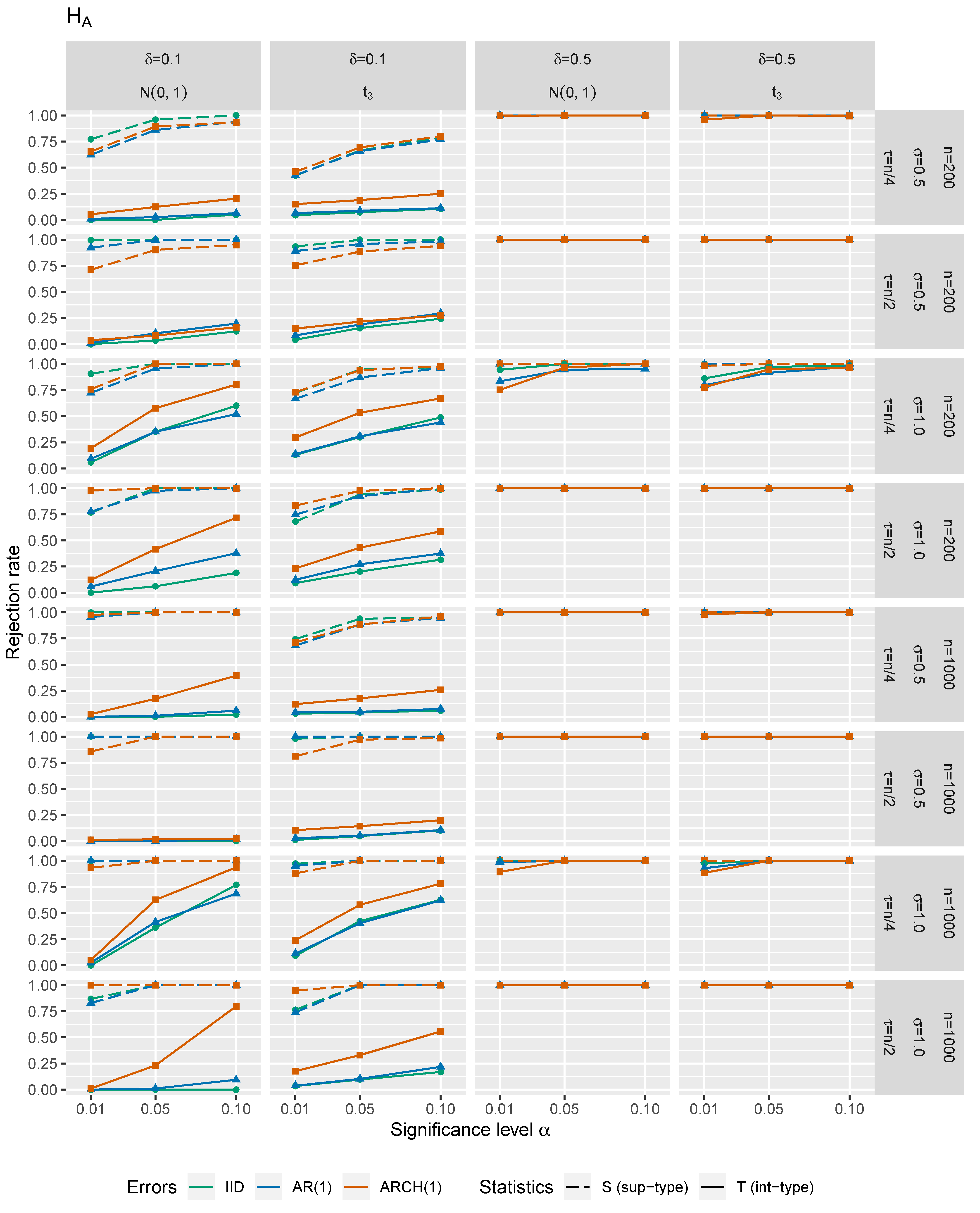
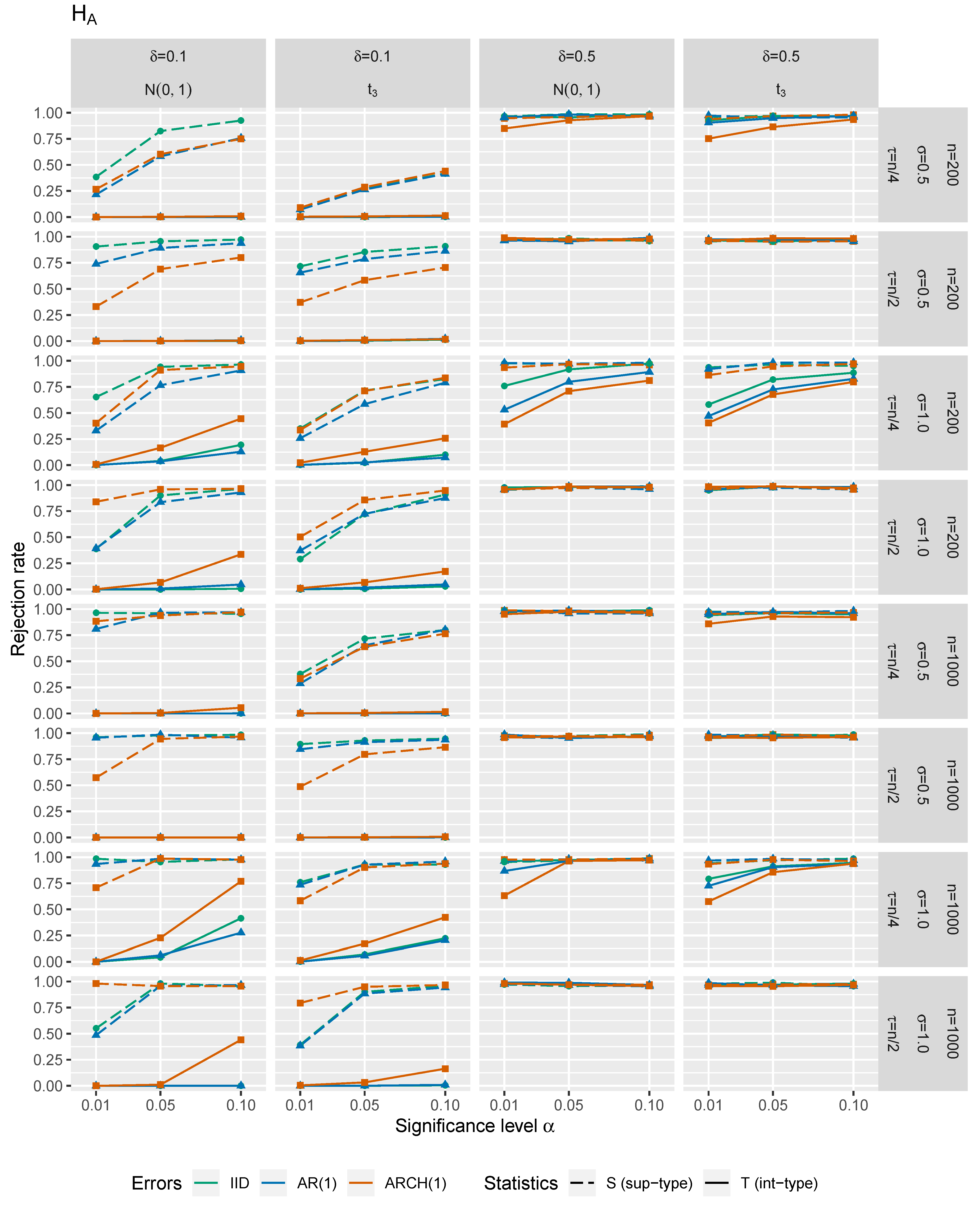
In Figure 1, Figure 2, Figure 3 and Figure 4, one may see size-power plots considering the test statistics and under the null hypothesis and under the alternative. Figure 1 and Figure 2 correspond to one input covariate (i.e., ) with choices of and . A case with four error-prone regressors (i.e., ) is illustrated in Figure 3 and Figure 4 for choices of and . Next, and . The size of change is for and for . Especially smaller values of the break should represent the situations under the local alternatives. In Figure 1 and Figure 3, the empirical rejection frequency under the null hypothesis (actual -errors) is plotted against the theoretical size (theoretical -errors with ), illustrating the size of the tests. The ideal situation under the null hypothesis is depicted by the straight diagonal dotted line. The empirical rejection frequencies (errors of the second type) under the alternative (with different changepoints and values of the change) are shown in Figure 2 and Figure 4, illustrating the power of the tests. Under the alternative, the desired situation would be a steep function with values close to 1. For more details on the size-power plots we may refer, e.g., to [47]. The standard deviation of the random disturbances was set to and the random error terms , and were independently simulated as three time series:
- IID … independent and identically distributed random variables;
- AR(1) … autoregressive (AR) process of order one with a coefficient of autoregression equal ;
- ARCH(1) … autoregressive conditional heteroscedasticity (ARCH) process with the second coefficient equal .
The standard normal distribution and the Student t-distribution with 3 degrees of freedom are used for generating the innovations of the models’ errors. All of the time series are standardized such that they have variance equal . Let us remark that the setup of Student -distribution does not satisfy Assumption . However, it can be considered to be a misspecified model and one would like to inspect performance of our procedures on such a model that violates our assumptions. In the simulations of the rejection rates, we used 10,000 repetitions.
In all of the subfigures of Figure 1 and Figure 3 depicting a situation under the null hypothesis, we may see that comparing the accuracy of -levels (sizes) for different self-normalized test statistics, the integral-type (-based) method seems to keep the theoretical significance level more firmly than the supremum-type (-based) method. Comparing the case of innovations with the case of innovations, the rejection rates under the null tend to be slightly higher for the -distribution. Despite the fact that the -distributed errors violate Assumption , the performance of our tests is still surprisingly satisfactory in such case. As expected, the accuracy of the critical values tends to be better for larger n and smaller p. The more complicated dependence structure of errors is assumed, the worse performance of the tests is obtained. Furthermore, the less volatile errors are set, the better tests’ sizes are attained.
The -method performs better under the null. However under the alternative, the -method has a tendency to have slightly higher power than the -method (see Figure 2 and Figure 4). We may also conclude that under with less volatile errors, the power of the test increases. The power decreases when the changepoint is closer to the beginning or the end of the input-output data. The heavier tails ( against ) give worse results in general for both test statistics. Moreover, ‘more dependent’ scenarios reveal worsening of the test statistics’ performance. Furthermore, the smaller size of the change is considered, the lower power of the test is achieved. In addition, again, the power gets higher for smaller p and larger n.
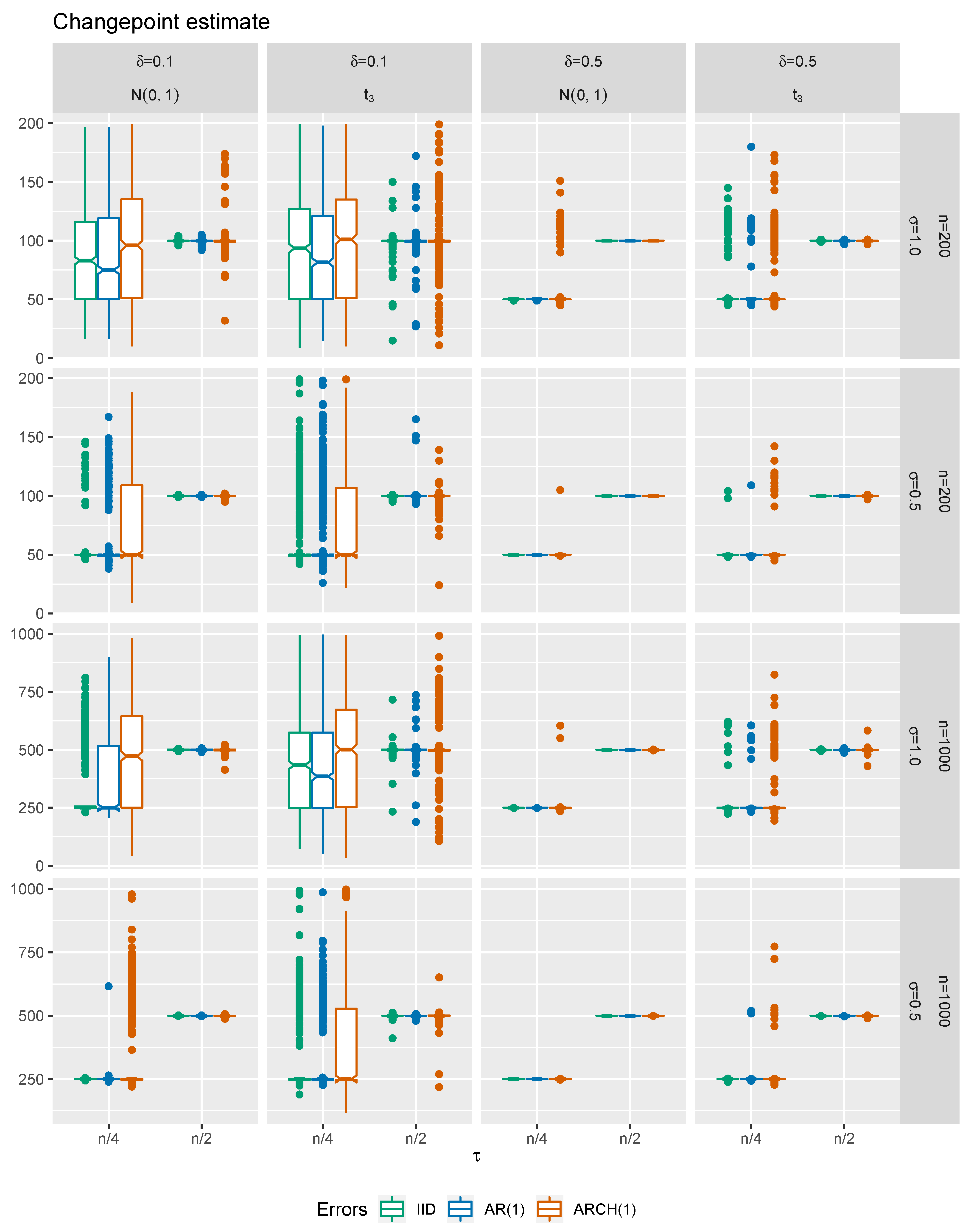
Afterwards, a simulation experiment is performed to study the finite sample properties of the changepoint estimator for a change in the linear relations’ parameter. We numerically present only the case of . In particular, the interest lies in the empirical distributions of the proposed estimator visualized via boxplots, see Figure 5 (bars correspond to the interquartile range). The simulation setup is kept the same as described above.
It can be concluded that the precision of our changepoint estimate is satisfactory even for relatively small sample sizes regardless of the errors’ structure. Less volatile model errors provide more precise changepoint estimate. The less complicated dependence structure is assumed, the higher accuracy of the estimator is obtained. Furthermore, the disturbances with heavier tails yield less precise estimates than innovations with light tails. One may notice that higher precision is obtained when the changepoint is closer to the middle of the data. It is also clear that the precision of improves markedly as the size of change increases.
6. Applications
6.1. Device Calibration
A company has two industrial devices, where the first one is calibrated according to some institute of standards and the second one is just a casual device. We want to test whether the second device is calibrated according to the first one. In this calibration problem, it means to know whether the second device has approximately the same performance up to some unknown multiplication constant as the first one. Consequently, other devices of the same type are needed to be calibrated as well. For some reasons, e.g., economic or logistic, it is only possible to calibrate one device by the official authorities.
Our data set, provided by a Czech steelmaker, contains 100 couples of speed values of two hammer rams (see Figure 6), where the first forging hammer is calibrated. We set the same power level on both hammers and measure the speed of each hammer ram repeatedly changing only the power level. Our measurements of the speed are encumbered with errors of the same variability in both cases, because we use the same device for measuring the speed and both forging hammers are of the same type. Since the power set for the forging hammer is directly proportional to the speed of the hammer ram, our goal is to test whether the ratio of two hammer rams’ speeds is kept constant over changing the power level or not. Therefore, our changepoint in the EIV model is very suitable for this setup—a linear dependence and errors in both measured speeds (with the same variance).
Both our changepoint tests— and —reject the null hypothesis of a constant linear coefficient between two hammer rams’ speed values at the significance level of (cf. Table 1), indicating a changed performance of the second non-calibrated hammer ram, although there is no visible change in trend present—the left part of Figure 6.
As an estimate for our change, we obtain (depicted by a vertical line in Figure 6—right), which corresponds to the 60th measurement of pair of speeds. After this particular measurement, we have background information that a technical issue appeared to the second hammer ram—one of its oil tubes started to leak. Our procedure is indeed capable of detecting and, consequently, estimating the (hardly visible, but present) changepoint in the ratio of the hammer rams’ speeds. In addition, this is done fully automatically without expert knowledge about the oil tube issue and also without setting tuning parameters. Moreover, the estimated ratio via the TLS approach before the change is (the slope of the green line in Figure 6), which basically says that the hammer rams work approximately in the same way. However, the estimated ratio via the TLS approach after the change is (the slope of the red line in Figure 6), which is significantly different from constant 1 (see a formal statistical test from [22]). In contrast, a significant change in trend is not detected using the ratio type changepoint test for the regression parameter [48]. A possible reason could be that such a detection approach misleadingly considers the covariates as error-free (i.e., measured precisely).
6.2. Randomly Spaced Time Series in Insurance
An insurance company records developments of the paid claim amounts coming from car accidents over time. Two types of claims with respect to car insurance are considered: material damage and bodily injury. The interest lies in disorder recognition between aggregated claim amounts paid for these two types of claims comprising two lines of insurance business.
Two claims (material damage and bodily injury) can come of one car accident and the corresponding claim amounts are expected to be related. We possess a data set from the Guarantee Fund of the Czech Insurers’ Bureau for car insurance. The aggregated claim amounts from the bodily injuries are monitored every time after the aggregated claim payments from the material damages exceed a threshold of CZK 2.5M (≈€100,000). This is performed by the bureau from the beginning of 2018 up to the end of 2019. The observation times () of the cumulative bodily injury claim amounts are random and irregularly spaced, because these time points are driven by a series of the cumulative material damage claim amounts.
Identification of structural breaks in the claim amounts and their development helps us to tie in specific legal, economic, or natural changes to the time epochs in which they occurred [49,50,51]. Our task is to test whether there is a common linear time trend of the cumulative bodily injury claim amounts or this trend has abruptly changed inside the monitoring regime [52,53,54,55]. Both our changepoint tests— and —reject the null hypothesis of a constant linear trend at the significance level of (cf. Table 1), indicating a changed payment development of the bodily injury claims.
As an estimate for the change, we obtain (depicted by a vertical line in Figure 7), which corresponds to 18 April 2019. The bureau for car insurance set some regulatory procedures forcing the insurance companies to change their reporting policy since the second quarter of 2019. This can result in a change of the bodily injury claim payments’ development and our detection procedures automatically reveal such regime switching. Additionally to that, Easter 2019 could also contribute to the change in the claim amounts. For example, Easter customs in the Central Europe and occasional drivers after the winter period cause more car accidents in general.
The data were firstly re-scaled in order to reach a common empirical variance yielding satisfiable Assumption and, then, inversely transformed back. The estimated linear time trend via the TLS approach before the change is (the slope of the green line in Figure 7) and after the change becomes (the slope of the red line in Figure 7). In contrast, a significant change in trend is not detected using the ratio type changepoint test for the regression parameter [48]. Again, a possible explanation could be that such a traditional detection approach misleadingly considers the time points as deterministic and error-free.
7. Conclusions
Our changepoint problem in linear relations is linearly defined, but comes with a highly non-linear solution and inference. We have proposed two tests for changepoints with desirable theoretical properties: The asymptotic size of the tests is guaranteed by a limit theorem even under non-stationarity and weak dependency; the tests and the related changepoint estimator are consistent. We are not aware of any similar results even for independent and identically distributed errors. By combining self-normalization and the proposed spectral weak invariance principle, there are neither tuning constants nor nuisance parameters involved in the whole testing procedure. Unknown or changing covariance structure of the errors is allowed. Therefore, the detection methods are completely data-driven, which makes this framework effortlessly applicable as demonstrated. In our simulations, the tests show reliable performance. Practical implementations of the developed detection techniques are demonstrated on two problems from calibration and insurance.
Funding
This research was supported by the Czech Science Foundation project GAČR No. 18-01781Y.
Institutional Review Board Statement
Not applicable.
Informed Consent Statement
Not applicable.
Data Availability Statement
The datasets presented in this study are available on request from the author. The data are not publicly available due to commercial issues.
Acknowledgments
The author would like to thank two anonymous referees for careful reading of the paper and for providing suggestions that improved this paper.
Conflicts of Interest
The author declares no conflict of interest.
Appendix A. Proofs
Proof of Proposition 1.
Let the singular value decomposition of the transformed ‘partial’ data matrix be
for some . Please note that we are in a situation of no change in the parameter . Bearing in mind Assumptions and , Lemma 2.1 in [1] and Theorem 3.1 in [20] provide that (i.e., the last element of the last right-singular vector corresponding to the smallest singular value) with probability tending to one as n increases. According to proof of Lemma 4.2 in [1], one gets
where is the TLS estimator for the transformed data and, additionally, . With respect to [20], we have
almost surely as . Moreover, as by [56]. The strong law of large numbers for -mixing by [57] together with Theorem 3.1 by [20] lead to almost surely. Since Assumption holds, the expression in (A2) is . Furthermore, the expression on the right hand side of (A1) is away from
as . Hence, the process from the left hand side of (A1) in has approximately the same distribution as the process (A3).
Please note that
Using the functional central limit theorem for -mixing by [58] or Corollary 3.2.1 in [59] in an analogous fashion as in the proof of Theorem 2.3 by [56], one gets
due to Assumption .
Similarly for and . ☐
Proof of Theorem 1.
The SWIP (Proposition 1) and Lemma 1 from [60] in combination with the continuous mapping device complete the proof. ☐
Proof of Theorem 2.
Under , let us find a lower bound for the smallest eigenvalue of the positive semi-definite matrix
where . With respect to Theorem 1 in [61], we get
where ℓ is any lower bound on the smallest eigenvalue of the matrix . Recall that Assumption and the proof of Theorem 3.1 by [20] provide
almost surely as , where and
By Assumptions
and
, one can obtain
almost surely as . Relation (A7) immediately provides a limit of a candidate for ℓ. Now, (A4) and (A5) lead to
Assumptions
,
, and relations (A6) yield
and
almost surely as . Thus,
almost surely as . Hence, combining (A8) and (A9) ends up with
Then,
by Assumption .
With respect to Assumptions , , and according to the underlying proof of Theorem 1, and are as . Moreover, as due to Proposition 1.
Please note that there are no changes in the linear parameter corresponding to the first observations as well as to the last (remaining) observations. Let . Thus, under
,
because of (A10).
Furthermore, again under ,
because of similar arguments as in the case of . ☐
Proof of Remark 1.
Proof of Corollary 1.
First of all, let us define ,
The estimator can be rewritten as
We will treat the numerator and the denominator of the above stated ratio separately. Let us use notations from the previous proofs and let us recall Assumption
,
, and relations (A6). If , then
almost surely as . Otherwise, if , then
almost surely as . In both cases, we have
where . Therefore, for the Frobenius matrix norm ,
uniformly in t almost surely, because due to proof of Lemma 2.3 in [21].
For , Proposition 1 together with the continuous mapping theorem yield that the denominator from (A11)
where the limit W is strictly positive almost surely. We conclude that converge in distribution to the random variable such that . For with , we obtain
according to the proof of Theorem 2 and assumption (10). The convergence holds uniformly for all t outside any right -neighborhood of . It follows that for an arbitrary ,
Similar arguments can be applied in the case . Assumption (11) provides, for an arbitrary ,
Relation (12) is equivalent to the statement that for every , there exists , such that . Thus, it is sufficient to show for any , there exists , such that
Proof of Lemma 1.
The relative Weyl theorem [63] applied on the multiplicative perturbation matrix provides
Then, realizing as completes the proof. ☐
Proof of Theorem 3.
Since are the linearly transformed original errors , the sequence is -mixing with the coefficients as due to [32]. Moreover, , and . Then, Assumption is satisfied for with . Theorem 2 and Corollary 1 can be applied to , where the resulting assertions hold for ’s and ’s instead of ’s and ’s, respectively.
Let us realize that as . Finally, it is sufficient to employ the relative Weyl theorem [63] and we get
Therefore, one can replace ’s and ’s by ’s and ’s, respectively, in the test statistics and changepoint estimator. ☐
References
- Gleser, L.J. Estimation in a multivariate “errors in variables” regression model: Large sample results. Ann. Stat. 1981, 9, 24–44. [Google Scholar] [CrossRef]
- Fuller, W.A. Measurement Error Models; Wiley: New York, NY, USA, 1987. [Google Scholar]
- Van Huffel, S.; Vandewalle, J. The Total Least Squares Problem: Computational Aspects and Analysis; SIAM: Philadelphia, PA, USA, 1991. [Google Scholar]
- Carroll, R.J.; Ruppert, D.; Stefanski, L.A.; Crainiceanu, C.M. Measurement Error in Nonlinear Models: A Modern Perspective, 2nd ed.; Chapman and Hall/CRC: Boca Raton, FL, USA, 2006. [Google Scholar]
- Buonaccorsi, J.P. Measurement Error: Models, Methods, and Applications; Chapman and Hall/CRC: Boca Raton, FL, USA, 2010. [Google Scholar]
- Yi, G.Y. Statistical Analysis with Measurement Error or Misclassification; Spriger: New York, NY, USA, 2017. [Google Scholar]
- Horváth, L. Detecting changes in linear regressions. J. Am. Stat. Assoc. 1995, 26, 189–208. [Google Scholar] [CrossRef]
- Aue, A.; Horváth, L.; Hušková, M.; Kokoszka, P. Testing for changes in polynomial regression. Bernoulli 2008, 14, 637–660. [Google Scholar] [CrossRef]
- Chang, Y.P.; Huang, W.T. Inferences for the linear errors-in-variables with changepoint models. J. Am. Stat. Assoc. 1997, 92, 171–178. [Google Scholar] [CrossRef]
- Staudenmayer, J.; Spiegelman, D. Segmented regression in the presence of covariate measurement error in main study/validation study designs. Biometrics 2002, 58, 871–877. [Google Scholar]
- Carroll, R.J.; Roeder, K.; Wasserman, L. Flexible parametric measurement error models. Biometrics 1999, 55, 44–54. [Google Scholar] [CrossRef]
- Gössl, C.; Küchenhoff, H. Bayesian analysis of logistic regression with an unknown change point and covariate measurement error. Statist. Med. 2001, 20, 3109–3121. [Google Scholar]
- Kukush, A.; Markovsky, I.; Van Huffel, S. Estimation in a linear multivariate measurement error model with a change point in the data. Comput. Stat. Data Anal. 2007, 52, 1167–1182. [Google Scholar]
- Dong, C.; Tan, C.; Jin, B.; Miao, B. Inference on the change point estimator of variance in measurement error models. Lith. Math. J. 2016, 56, 474–491. [Google Scholar] [CrossRef]
- Booth, J.G.; Hall, P. Bootstrap confidence regions for functional relationships in errors-in-variables models. Ann. Stat. 1993, 21, 1780–1791. [Google Scholar]
- Stefanski, L.A. Measurement error models. J. Am. Stat. Assoc. 2000, 95, 1353–1358. [Google Scholar] [CrossRef]
- Golub, G.H.; Van Loan, C.F. An analysis of the total least squares problem. SIAM J. Numer. Anal. 1980, 17, 883–893. [Google Scholar] [CrossRef]
- Pešta, M. Unitarily invariant errors-in-variables estimation. Stat. Pap. 2016, 57, 1041–1057. [Google Scholar] [CrossRef]
- Gallo, P.P. Consistency of regression estimates when some variables are subject to error. Commun. Stat. A-Theor. 1982, 11, 973–983. [Google Scholar] [CrossRef] [Green Version]
- Pešta, M. Strongly consistent estimation in dependent errors-in-variables. Acta Univ. Carol. Math. Phys. 2011, 52, 69–79. [Google Scholar]
- Gallo, P.P. Properties of Estimators in Errors-in-Variables Models. Ph.D. Thesis, University of North Carolina, Chapel Hill, NC, USA, 1982. [Google Scholar]
- Pešta, M. Total least squares and bootstrapping with application in calibration. Statistics 2013, 47, 966–991. [Google Scholar] [CrossRef]
- Pešta, M. Block bootstrap for dependent errors-in-variables. Commun. Stat. A-Theor. 2017, 46, 1871–1897. [Google Scholar] [CrossRef]
- Bland, J.M.; Altman, D.G. Statistical methods for assessing agreement between two methods of clinical measurement. Lancet 1986, 1, 307–310. [Google Scholar] [CrossRef]
- Lord, F.M. Testing if two measuring procedures measure the same dimension. Psychol. Bull. 1973, 79, 71–72. [Google Scholar] [CrossRef]
- Wright, D.J. Forecasting data published at irregular time intervals using an extension of Holt’s method. Manag. Sci. 1986, 32, 499–510. [Google Scholar] [CrossRef]
- Gleser, L.J.; Watson, G.S. Estimation of a linear transformation. Biometrika 1973, 60, 525–534. [Google Scholar] [CrossRef]
- Ryu, S.J.; Lee, H.K. Estimation of linear transformation by analyzing the periodicity of interpolation. Pattern Recogn. Lett. 2014, 36, 89–99. [Google Scholar] [CrossRef]
- Ochoa, J.; León, A.; Ramírez, I.; Lopera, C.; Bernal, E.; Arbeláez, M. Prevalence of tuberculosis infection in healthcare workers of the public hospital network in Medellín, Colombia: A Bayesian approach. Epidemiol. Infect. 2017, 145, 1095–1106. [Google Scholar] [CrossRef] [Green Version]
- Hosseini, M.; Jiang, Y.; Yekkehkhany, A.; Berlin, R.R.; Sha, L. A mobile geo-communication dataset for physiology-aware DASH in rural ambulance transport. In Proceedings of the 8th ACM on Multimedia Systems Conference (MMSys’17); Association for Computing Machinery: New York, NY, USA, 2017; pp. 158–163. [Google Scholar] [CrossRef] [Green Version]
- Li, M.; Liu, Z.; Li, X.; Liu, Y. Dynamic risk assessment in healthcare based on Bayesian approach. Reliab. Eng. Syst. Saf. 2019, 189, 327–334. [Google Scholar] [CrossRef]
- Bradley, R.C. Basic properties of strong mixing conditions. A survey and some open questions. Probab. Surv. 2005, 2, 107–144. [Google Scholar] [CrossRef] [Green Version]
- Anderson, T.W. An Introduction to Multivariate Statistical Analysis; John Wiley & Sons: New York, NY, USA, 1958. [Google Scholar]
- Billingsley, P. Convergence of Probability Measures, 1st ed.; John Wiley & Sons: New York, NY, USA, 1968. [Google Scholar]
- Ibragimov, I.A.; Linnik, Y.V. Independent and Stationary Sequences of Random Variables; Wolters-Noordhoff: Groningen, The Netherlands, 1971. [Google Scholar]
- Rosenblatt, M. Markov Processes: Structure and Asymptotic Behavior; Springer: Berlin, Germany, 1971. [Google Scholar]
- Cheng, C.L.; Riu, J. On estimating linear relationships when both variables are subject to heteroscedastic measurement errors. Technometrics 2006, 48, 511–519. [Google Scholar] [CrossRef]
- Guo, Y.; Little, R.J. Regression analysis with covariates that have heteroscedastic measurement error. Statist. Med. 2011, 30, 2278–2294. [Google Scholar] [CrossRef] [PubMed]
- Li, M.; Ma, Y.; Li, R. Semiparametric regression for measurement error model with heteroscedastic error. J. Multivar. Anal. 2019, 171, 320–338. [Google Scholar] [CrossRef]
- Nussbaum, M. Asymptotic optimality of estimators of a linear functional relation if the ratio of the error variances is known. Statistics 1977, 8, 173–198. [Google Scholar]
- Kao, C.; Trapani, L.; Urga, G. Testing for instability in covariance structures. Bernoulli 2018, 24, 740–771. [Google Scholar] [CrossRef] [Green Version]
- Van Huffel, S.; Vandewalle, J. Analysis and properties of the generalized total least squares problem AX ≈ B when some or all columns in A are subject to error. SIAM J. Matrix Anal. Appl. 1989, 10, 294–315. [Google Scholar] [CrossRef]
- Shao, X.; Zhang, X. Testing for change points in time series. J. Am. Stat. Assoc. 2010, 105, 1228–1240. [Google Scholar] [CrossRef]
- Csörgo, M.; Horváth, L. Limit Theorems in Change-Point Analysis; Wiley: Chichester, UK, 1997. [Google Scholar]
- Fang, H.; Ding, S.; Li, X.; Yang, W. Asymptotic approximations of ratio moments based on dependent sequences. Mathematics 2020, 8, 361. [Google Scholar] [CrossRef] [Green Version]
- Ding, S.; Li, X.; Dong, X.; Yang, W. The consistency of the CUSUM-type estimator of the change-point and its application. Mathematics 2020, 8, 2113. [Google Scholar] [CrossRef]
- Kirch, C. Resampling Methods for the Change Analysis of Dependent Data. Ph.D. Thesis, University of Cologne, Cologne, Germany, 2006. [Google Scholar]
- Peštová, B.; Pešta, M. Variance estimation free tests for structural changes in regression. In Nonparametric Statistics; Bertail, P., Blanke, D., Cornillon, P.A., Matzner-Løber, E., Eds.; Springer: Cham, Switzerland, 2018; Volume 250, pp. 357–373. [Google Scholar]
- Pešta, M.; Hudecová, Š. Asymptotic consistency and inconsistency of the chain ladder. Insur. Math. Econ. 2012, 51, 472–479. [Google Scholar] [CrossRef]
- Hudecová, Š.; Pešta, M. Modeling Dependencies in Claims Reserving with GEE. Insur. Math. Econ. 2013, 53, 786–794. [Google Scholar] [CrossRef] [Green Version]
- Pešta, M.; Okhrin, O. Conditional least squares and copulae in claims reserving for a single line of business. Insur. Math. Econ. 2014, 56, 28–37. [Google Scholar] [CrossRef] [Green Version]
- Peštová, B.; Pešta, M. Change point estimation in panel data without boundary issue. Risks 2017, 5, 7. [Google Scholar] [CrossRef]
- Maciak, M.; Peštová, B.; Pešta, M. Structural breaks in dependent, heteroscedastic, and extremal panel data. Kybernetika 2018, 54, 1106–1121. [Google Scholar] [CrossRef]
- Pešta, M.; Peštová, B.; Maciak, M. Changepoint estimation for dependent and non-stationary panels. Appl. Math-Czech 2020, 65, 299–310. [Google Scholar] [CrossRef]
- Maciak, M.; Pešta, M.; Peštová, B. Changepoint in dependent and non-stationary panels. Stat. Pap. 2020, 61, 1385–1407. [Google Scholar] [CrossRef]
- Pešta, M. Asymptotics for weakly dependent errors-in-variables. Kybernetika 2013, 49, 692–704. [Google Scholar]
- Chen, X.; Wu, Y. Strong law for mixing sequence. Acta Math. Appl. Sin. 1989, 5, 367–371. [Google Scholar] [CrossRef]
- Herrndorf, N. Stationary strongly mixing sequences not satisfying the central limit theorem. Ann. Probab. 1983, 11, 809–813. [Google Scholar] [CrossRef]
- Lin, Z.; Lu, C. Limit Theory for Mixing Dependent Random Variables; Springer: New York, NY, USA, 1997. [Google Scholar]
- Pešta, M.; Wendler, M. Nuisance-parameter-free changepoint detection in non-stationary series. TEST 2020, 29, 379–408. [Google Scholar] [CrossRef]
- Dembo, A. Bounds on the extreme eigenvalues of positive-definite Toeplitz matrices. IEEE Trans. Inform. Theory 1988, 34, 352–355. [Google Scholar] [CrossRef]
- Ma, E.M.; Zarowski, C.J. On lower bounds for the smallest eigenvalue of a Hermitian positive-definite matrix. IEEE Trans. Inform. Theory 1995, 41, 539–540. [Google Scholar] [CrossRef]
- Nakatsukasa, Y. Absolute and relative Weyl theorems for generalized eigenvalue problems. Linear Algebra Appl. 2010, 432, 242–248. [Google Scholar] [CrossRef] [Green Version]
Figure 1.
Size-power plots for and under
().

Figure 2.
Size-power plots for and under ().

Figure 3.
Size-power plots for and under ().

Figure 4.
Size-power plots for and under ().

Figure 5.
Boxplots of the estimated changepoint ().

Figure 6.
Speeds of two hammer rams, where the first one displayed on the x-axis is calibrated—without (left) and with (right) the estimated trend. The changepoint estimate corresponding to the technical issues is depicted by the vertical line.
Figure 6.
Speeds of two hammer rams, where the first one displayed on the x-axis is calibrated—without (left) and with (right) the estimated trend. The changepoint estimate corresponding to the technical issues is depicted by the vertical line.

Figure 7.
Cumulative claim amounts (y-axis) at unequally spaced non-deterministic time points (x-axis). The detected changepoint of the time trend is depicted by the vertical line.
Figure 7.
Cumulative claim amounts (y-axis) at unequally spaced non-deterministic time points (x-axis). The detected changepoint of the time trend is depicted by the vertical line.


Table 1.
Simulated asymptotic critical values for and .
| -based | |||||
| -based |
Publisher’s Note: MDPI stays neutral with regard to jurisdictional claims in published maps and institutional affiliations. |
© 2021 by the author. Licensee MDPI, Basel, Switzerland. This article is an open access article distributed under the terms and conditions of the Creative Commons Attribution (CC BY) license (http://creativecommons.org/licenses/by/4.0/).
Share and Cite
MDPI and ACS Style
Pešta, M. Changepoint in Error-Prone Relations. Mathematics 2021, 9, 89. https://doi.org/10.3390/math9010089
AMA Style
Pešta M. Changepoint in Error-Prone Relations. Mathematics. 2021; 9(1):89. https://doi.org/10.3390/math9010089
Chicago/Turabian StylePešta, Michal. 2021. "Changepoint in Error-Prone Relations" Mathematics 9, no. 1: 89. https://doi.org/10.3390/math9010089
Note that from the first issue of 2016, this journal uses article numbers instead of page numbers. See further details here.