Dealing with Degeneracies in Automated Theorem Proving in Geometry

Abstract

We report, through different examples, the current development in GeoGebra, a widespread Dynamic Geometry software, of geometric automated reasoning tools by means of computational algebraic geometry algorithms. Then we introduce and analyze the case of the degeneracy conditions that so often arise in the automated deduction in geometry context, proposing two different ways for dealing with them. One is working with the saturation of the hypotheses ideal with respect to the ring of geometrically independent variables, as a way to globally handle the statement over all non-degenerate components. The second is considering the reformulation of the given hypotheses ideal—considering the independent variables as invertible parameters—and developing and exploiting the specific properties of this zero-dimensional case to analyze individually the truth of the statement over the different non-degenerate components.

1. Introduction

This paper deals with some issues related to the successful approach to the automated verification and derivation of theorems in elementary geometry through computational algebraic geometry techniques, initiated more than forty years ago by Wu [1].

The relatively recent implementation of geometric automated reasoning tools (GART) on Dynamic Geometry programs (See https://en.wikipedia.org/wiki/List_of_interactive_geometry_software, accessed on 13 August 2021, for a table providing a list of the different Dynamic Geometry programs with automated proving features.), allowing the algorithmic verification and derivation of geometric theorems, has renewed the interest in analyzing—and handling—some problems arising in the underlying interaction of the different pieces involved in the GART protocols. In particular, we refer to the quite successful performance of such tools in the Dynamic Geometry program GeoGebra (https://www.geogebra.org/download, accessed on 13 August 2021), freely available and with over one hundred million users all over the world, a fact that has reinforced and urged the need to address some pending problems.

In this paper we begin by illustrating, through a collection of examples, the current performance and ongoing development of GART in GeoGebra and its algebraic geometry background (see Section 2 and Section 3). Then we reflect (Section 4) on some (unexpected for a standard user) problems that might arise, due to the interaction of the different steps involved in the process, such as the user specific interpretation and introduction of the geometric statement, the internal algebraic translation, and the algorithmic manipulation of polynomial ideals towards the final output (and again, its interpretation by the user).

Finally, we focus on a particular kind of such problems (Section 5), proposing a double approach that might help to avoid featuring counterintuitive conclusions due to unexpected degenerate instances of the given hypotheses (Section 6). One is to deal with the saturation of the hypotheses ideal with respect to the ring of geometrically independent variables, thus allowing for the global consideration of the given statement over all non-degenerate components. The second is to reformulate the hypotheses ideal by treating the independent variables as invertible parameters, showing the specific advantages of this zero-dimensional case to analyze individually the truth of the statement over the different non-degenerate components. The paper concludes with some reflections on the potential application of these methods.

2. Automated Reasoning Tools in GeoGebra

As described in [2,3], the standard version of GeoGebra includes now several commands:

• For conjecturing some geometric property (e.g., “...these three lines visually “seem” to meet at one point. Is this actually true?...”);
• For rigorously confirming or denying a proposed conjecture (e.g., yielding an affirmative answer after internally verifying, using Computer Algebra tools, that the equations describing the three selected lines have always a common solution);
• For suggesting some complementary hypotheses for the truth of a given (initially false) statement (i.e., declaring some further restrictions in the geometric elements involved in the statement, that are required for its verification).

2.1. The Altitude Theorem

Let us consider the classical “Geometric Mean” or “Altitude” Theorem attributed to Euclid (see [4], pp. 31–32). The traditional formulation states that in a right triangle, the length of the altitude on the hypotenuse is equal to the geometric mean of the two line segments it creates on the hypotenuse. However, suppose we “forget” about the condition to be a right triangle, yet we would like to remember the missing hypothesis, in order to rediscover this classic theorem. Then, we could start by conjecturing the truth of this theorem on a general triangle. Next, that of GART, the Prove command, declares (see Figure 1) it is wrong.

Now, we ask for the requirements to place vertex C so that the Altitude Theorem holds. GeoGebra outputs two curves: a circle and a hyperbola (see Figure 2, left image). Clearly, the first one corresponds to the right triangle case, that is, verifying that the sum of the two angles of the triangle at vertices $A,B$ is 90 degrees; the second places C at some hyperbola. We have, thus, obtained two possible versions of the Altitude Theorem: the traditional one and the one corresponding to triangles $ABC$ with C in the given hyperbola. As the equation of the hyperbola is given by GeoGebra, we can play a little with it (in a non-automatic way) concluding that such triangles are precisely those such that the difference of angles at $A,B$ is also 90 degrees.

Moreover, we can perform a specific construction of such triangles from a given pair of vertices $A,B$, placing point C at the hyperbola as follows (Figure 2, right): first, choosing an arbitrary point G, considering the line $f_1=GA$, a perpendicular line through B, and its symmetrical $h^{\prime }$ with respect to the $AB$ line. Then C is the intersection of $f_1,h^{\prime }$. See [5] for details about this construction and generalized Altitude Theorem statement.

Figure 2, right image, shows how GeoGebra checks the truth of this extended version of the Altitude Theorem, yielding true as the Boolean Value corresponding to the question Prove $(g^2==h·i)$, where g is the segment described by the altitude from vertex C and $h,i$ are the segments $DA,DB$, respectively, going from the altitude feet D in the line $AB$, to the vertices $A,B$.

2.2. A problem from a Spanish ‘Oposiciones’ Exam

A different example of the performance of GeoGebra’s automated reasoning tools is displayed in Figure 3. Given a quadrilateral $ABCD$, the midpoints $E,F,G,H$ of the sides are built. Then GeoGebra is asked to find (left image) a Relation holding between the segments $EF,GH$. In the central image we can see that GeoGebra replies that the lengths of the two segments seem to be equal, at least numerically and for this particular assignment of the vertices of the quadrilateral. Thus, the user might conjecture that, perhaps, this fact holds in all generality, as a geometric statement. To check this conjecture, the user has to click on the More... button. Then GeoGebra launches internally the Prove command, yielding that it is indeed true (except for degenerate instances of the given construction) that the midpoints of the sides of the quadrilateral always form a parallelogram.

However, the ability of the Relation command to find conjectures goes well beyond simple, school-like contexts. For example, in [6] it is shown how GeoGebra’s Relation is able to automatically conjecture and, then, prove, the alignment of some three points stated in Example 230 of the classical Chou’s benchmark [7]. Another, quite curious, case is depicted in Figure 4, that shows two further examples of the powerful performance of the Relation command. The context is a problem proposed at a Spanish national exam ([8], p. 147) to become a certified mathematics teacher for secondary education. The candidates were given (on the exam sheet) a complicated figure that we can translate to a GeoGebra construction as follows (see Figure 4). First, consider an equilateral triangle $ABC$, and build E, the midpoint of side $AB$, and D, the midpoint of $AC$. Then construct $B^{\prime }$, the symmetrical of B with respect to D, and $B_1^{\prime }$, the symmetrical of B with respect to A. Next, label the altitude from C as a, b is side $BC$, e is segment $AD$ and m is the segment $AF$, where F is the intersection of $B_1^{\prime }D$ and $B^{\prime }E$. Finally, the candidates to become an official mathematics teacher were asked to find out the existing relation between $t=DC$ and $m=AF$. So as not to spoil the intrigued reader about this question, we refer to [9] where it is fully answered using only GeoGebra automated reasoning tools.

Yet, we would like to show here, over the same construction from the Spanish exam, the answer to two much more complicated queries, showing, in particular, that GeoGebra’s Relation is suitable for finding relations involving algebraic numbers. Thus, Figure 4, left image, displays the result of asking about the relation between $a+b$ and e, that happens to be $a+b=(2+\sqrt{3})/2·e$; the right image corresponds to the relation between a and m, yielding $a=1/2·\sqrt{21}·m$. It must be remarked that these answers were obtained almost immediately with a MacBookPro 2015, with 2.5 GHz Intel Core i7 processor.

2.3. Ongoing Work

Besides the Relation, Prove, ProveDetails and LocusEquation commands that we have summarily exemplified, let us briefly mention two other reasoning tools, already implemented in (yet) non-standard versions of GeoGebra [10,11]. The first one, the Discover tool and command, can be used in the GeoGebra Discovery fork (Available at https://github.com/kovzol/geogebra-discovery, http://autgeo.online/geogebra-discovery/, accessed on 13 August 2021), available in two different options: one, operating over GeoGebra Classic 5, for Windows, Mac and Linux systems; and, the other, working over GeoGebra Classic 6, that requires starting it in a browser, for tablets and smartphones.

For example, Figure 5 shows some of the new features in GeoGebra Discovery, the Discover command, that automatically finds—and illustrates by depicting some complementary geometric elements over the figure—all theorems (of a certain kind: parallelism, congruence, perpendicularity, etc.) holding over a given element of a construction (e.g., point E, in Figure 5). Roughly speaking, this command operates by considering some combinatorial heuristics to formulate different Relation tests involving always the selected element (here point E), plus some other ones, and presenting as output the collection of obtained properties.

The second ongoing improvement refers to the construction of AG=Automated Geometer (Available at http://autgeo.online/ag/, https://github.com/kovzol/ag, accessed on 13 August 2021), a self-operating ‘geometer’ (i.e., without requiring human intervention, except that of launching the computation process over a figure) within GeoGebra. It is a web-based module that allows GeoGebra to automatically formulate different geometric conjectures over the given input geometric construction and to confirm or deny them using internally tools similar to those in GeoGebra Discovery; however, here it is not limited to exploring relations involving a single, specific element, see Figure 6.

3. A Simplified Introduction to the Algebro-Geometric Background

As already mentioned in the Introduction, there is an ‘ad hoc’, computational (complex) algebraic geometry approach behind the performance of the different tools we have exemplified. Very roughly speaking (see [12] for the mathematical background, or [2] for further details regarding the different methods implemented in GeoGebra), GeoGebra proceeds by automatically translating the different steps of the construction involved in a given statement into a series of polynomial equations. Now, looking for the Relation between some elements of the corresponding figure is addressed by describing the result of eliminating, in this polynomial system, all variables except those associated to the selected elements.

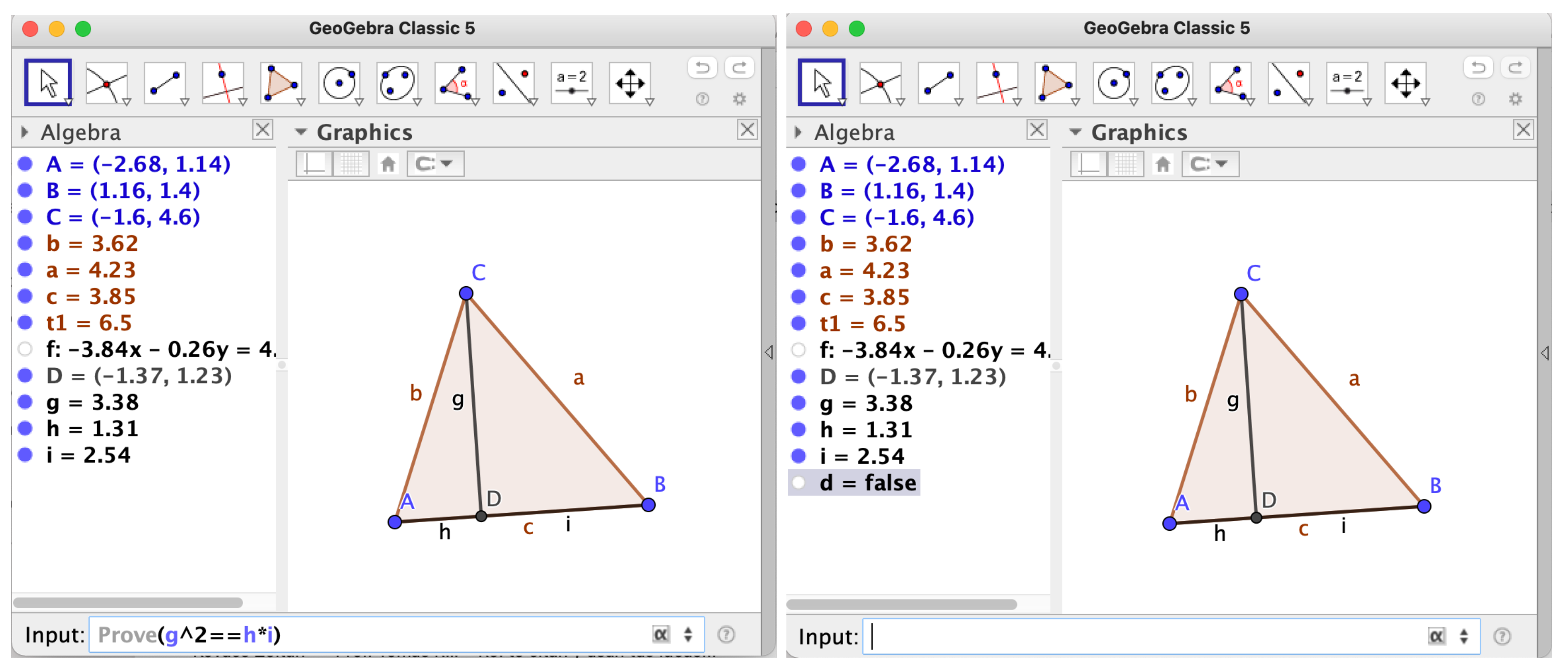
For instance, given a right triangle $ABC$, so that $AC$ and $BC$ are perpendicular, suppose we would like to find the relation between the altitude g of C and the pair of segments $h=AD,i=DB$, where D is the altitude foot on side $AB$, see Figure 1. Then GeoGebra can assume, for simplicity, that $A=(0,0),B=(1,0),C=(c_1,c_2)$, and it is likely to consider the following equation $c_1·(c_1-1)+c_2^2=0$ describing the perpendicularity of the two catheti $AC,BC$, and the equations (at least from an intuitive point of view) describing $g,h,i$: $\{g=c_2,h=c_1,i=1-c_1\}$. Finally, the elimination of $\{c_1,c_2\}$ in this system yields (among others) the equation $g^2=h·i$, that is, the Relation described in the Altitude Theorem.

On the other hand, if we already know the thesis $g^2=h·i$ of this theorem and we just want to verify that it holds always true on right triangles, by means of the Prove command, GeoGebra considers its refutation, which seems natural to be expressed through the system of equations

$$\{c_1·(c_1-1)+c_2^2=0,g-c_2=0,h-c_1=0,i-(1-c_1)=0,(g^2-h·i)·t-1=0\}$$

where the last one $(g^2-h·i)·t-1=0$ represents the negation of the thesis. Now it checks that this system has no solutions at all, i.e., that 1 is a combination of the given equations (by Hilbert’s Nullstellensatz). Thus, since it happens that the refutation of the introduced statement is never true, GeoGebra concludes that the statement is always true!

Finally, to provide a more complete, albeit very naive, description about the implemented algorithmic approach, let us assume, as in Figure 1, that we consider a general triangle and we would like to learn the conditions for the Altitude Theorem to hold. Here GeoGebra could proceed considering now the set of equations $\{g-c_2=0,h-c_1=0,$$i-(1-c_1)=0,g^2-h·i=0\}$, where we have dropped the perpendicularity requirement of the catheti and we have added the verification of the thesis $g^2-h·i=0$. Again, by elimination of all variables except $\{c_1,c_2\}$ we obtain the LocusEquation:$c_1^2+c_2^2-c_1=0$, i.e., that the truth of the thesis of the Altitude Theorem requires that C lies on the locus given by the circle of center the midpoint of $AB$, or, equivalently, that $ABC$ is a right triangle at C.

4. Complications

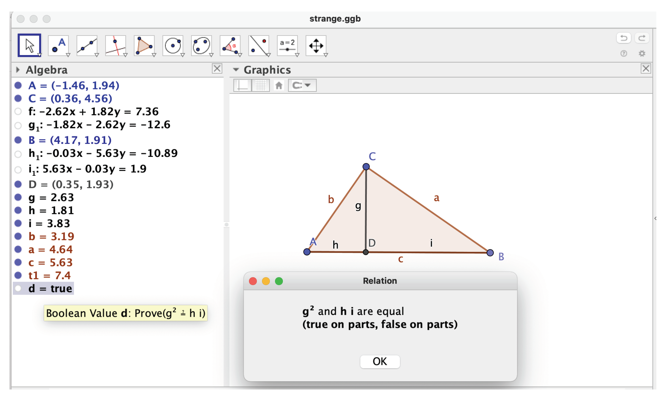
The conclusion of the last section seems to contradict the output of Figure 2, which included a hyperbola and a circle as the locus for the Altitude Theorem! Moreover, it happens that if the Relation tool is applied to verify the truth of this statement for a right triangle $ABC$, the output message is “true on parts, false on parts”. Even more confusing, this declaration contradicts the result of the Prove command, that declares the truth of the thesis $g^2-h·i=0$ (see Figure 7). This issue is specifically addressed in [13], and it is related to the fact that the—perhaps intuitively evident—equations that we have used here describing $g,h,i$:, i.e.,  $\{g=c_2,h=c_1,i=1-c_1\}$, are actually to be replaced, to work in all generality with lengths of segments, by $\{g^2={c_2}^2,h^2={c_1}^2,i^2={(1-c_1)}^2\}$ and, then, choosing the positive values of $g,h,i$.

It happens that, if we mimic the procedure described at the beginning of the previous section, with this new set of equations plus the perpendicularity condition $c_1·(c_1-1)+c_2^2=0$, the elimination of $\{c_1,c_2\}$ in this complete system yields now $\{g^4-h^2·i^2=(g^2-h·i)·(g^2+h·i)\}$, and not $g^2=h·i$. Therefore, in this new context, the thesis of the Altitude Theorem would not be obtained as output of the Relation command! Of course, the equality $g^2+h·i=0$ cannot hold for positive values of $g,h,i$ and, thus, $(g^2-h·i)·(g^2+h·i)=0$ is equivalent to $g^2=h·i$ for real positive values; however, working over the real numbers and involving inequalities requires replacing Gröbner-based elimination methods by real quantifier elimination algorithms, with weaker performance (see [14] for some very promising but preliminary results in this direction).

Thus, a different operating alternative has been developed in [15,16], observing that $g^2=h·i$ holds over some primary components of the variety described by the complex solutions of

$$\{g^2={c_2}^2,h^2={c_1}^2,i^2={(1-c_1)}^2,c_1·(c_1-1)+c_2^2=0\}$$

and fails over some others (where $g^2+h·i=0$ holds), i.e., the Altitude Theorem is “true on parts, false on parts” (as shown in Figure 7). Again, the idea is to arrive to such a conclusion without having to compute the (costly) primary decomposition.

This somehow confusing panorama: intuitive algebraic formulation, manipulation, and derivation of geometric facts vs. (sometimes) contradictory GeoGebra’s output, is just a warning sign of the need to revise the naive approach we have described in the previous section. As already remarked, to begin with, given a certain geometric situation, we should pay special attention to the way we introduce the algebraic input in the automated reasoning algorithms. Indeed, the automated reasoning protocol starts by having the human user translating the textual—or figural or imagined—context into a GeoGebra construction. This translation is not irrelevant. For instance, in the context of Thales theorem (https://en.wikipedia.org/wiki/Thales’s_theorem, accessed on 13 August 2021), if we want to deal with a circle c, a diameter $AB$, a point C on the circle and lines $CA,CB$, a possible approach could be to start fixing two points $O,A$, then building the circle centered at O and passing through A, choosing one point C on the circle and, finally, intersecting the circle with the line $OA$ to get the other extreme B of the diameter. This yields, with a straightforward translation (We exemplify the following computations using Maple computer algebra software, https://www.maplesoft.com, accessed on 13 August 2021), the following ideal of hypotheses:

$$Ideal1:={\langle (c_1-o_1)}^2+{(c_2-o_2)}^2-{(a_1-o_1)}^2-{(a_2-o_2)}^2,$$

$${(b_1-o_1)}^2+{(b_2-o_2)}^2-{(a_1-o_1)}^2-{(a_2-o_2)}^2,$$

$$(b_1-o_1)·(a_2-o_2)-(b_2-o_2)·(a_1-o_1)\rangle$$

with $\{o_1,o_2,a_1,a_2,c_1\}$ as free variables. Now, both adding the refutation of the thesis, the perpendicularity of $CA,CB$, i.e., $((c_1-b_1)·(c_1-a_1)+(c_2-b_2)·(c_2-a_2))·t-1$, or the thesis itself $(c_1-b_1)·(c_1-a_1)+(c_2-b_2)·(c_2-a_2)$, yields the zero ideal with eliminating all except the free variables. Thus the statement is ‘true on parts’ [15,16], that is, neither true nor false, because point B—the intersection of a line and a circle—is not uniquely defined and yields different primary components on the hypotheses ideal, some of them holding true, some false, the given thesis.

On the other hand, if the construction starts with two free points $A,B$ and considers the circle centered at the midpoint O of segment $AB$, a point C on the circle, and lines $CA,CB$, the corresponding ideal

$$Ideal2:={\langle (c_1-o_1)}^2+{(c_2-o_2)}^2-{(a_1-o_1)}^2-{(a_2-o_2)}^2,$$

$$o_1-(a_1+b_1)/2,o_2-(a_2+b_2)/2\rangle$$

has only one component and the perpendicularity of $CA,CB$ is always true on it:

• EliminationIdeal(<(c_1-o_1)^2+(c_2-o_2)^2-(a_1-o_1)^2-(a_2-o_2)^2,
• o_1-(a_1+b_1)/2, o_2-(a_2+b_2)/2,
• ((c_1-b_1)*(c_1-a_1)+(c_2-b_2)*(c_2-a_2))*t-1>,
• {a_1,a_2,b_1,b_2,c_1});
•                 <1>

Next to the impact of the human translation—through the choice of the construction steps—of a given statement, are the different assumptions and tricks that GeoGebra programmers have implemented in the involved algorithms, to speed up the automatic reasoning features. For instance, internally, the initial free points are usually assumed to be $(0,0),(1,0)$ in order to diminish the number of involved variables; in addition, some negative constraints, using Rabinowitsch’s trick, are often added to avoid foreseeable degeneracies, such as the coincidence of two points, but with potentially conflictive consequences [17]; likewise, to deal with magnitudes that are supposed to be positive, GeoGebra considers automatically only some specific components of the hypotheses variety or includes the so-called Minimal Euclidean Polynomial (MEP) extension, that represents only with even powers all variables related to distances [13], etc.

We refer, for precise details and examples to illustrate the difficulties and the adopted technical solutions, to the basic document [12] and, for recent updates, to [13,15] or [17]. The algorithms described in these papers are implemented in GeoGebra through the embedded computer algebra system Giac [18,19].

5. Reflecting about Degeneracy Conditions

One of the more frequent, yet unexpected, outputs of the automated reasoning tools is the inclusion of a list of degenerate cases (e.g., circles of radius zero, triangles collapsing to a line, etc.) in the answer to the ProveDetails command. Cases have to be avoided because of the generic truth of a certain statement that the user was ‘a priori’ convinced was absolutely true. This problem has been well known for a long time and happens even in quite simple cases (see [12]). For example, it might happen that the user had constructed a circle or a triangle, and GeoGebra had translated the construction into polynomial equations, but both the graphic and the algebraic counterpart include the case of the circle being reduced to a point. There is also the case of the three vertices of the triangle being aligned or coincident, etc., even if the user did not consider, intuitively, such instances as verifying the hypotheses of a certain geometric statement. Then, it can occur—somehow at random and with little geometric interpretation, since it might refer to the diameter of a circle of radius zero, or to the heights of a triangle reduced to a point, etc.—that some of these degenerate instances do not verify a given thesis, yielding thus a negative answer to the correctness of a proposition that the user reasonably considered as true.

To avoid as much as possible such situations, the algorithm in [12], quite successfully implemented in GeoGebra (see [2,3]), considers as ‘generally true’ those statements where the thesis vanishes over all the irreducible components of the hypotheses variety describing all the non-degenerate instances; i.e., it disregards, as irrelevant that the thesis fails over the components that include degenerate cases. Likewise, a statement is labeled as ‘generally false’ if the thesis does not vanish identically over every non-degenerate irreducible component of the hypotheses variety—those describing the non-degenerate instances; it does not matter that the thesis holds over the components that include degenerate cases. Thus, it turns out that the key concept is that of ‘degeneracy’.

The usual approach to deal with this issue is, first, to consider that the different steps of a construction provide a collection of points that rule the construction, i.e., that, if dragged along the window of the application, the whole construction should follow them. For example, in Figure 1, the three vertices $A,B,C$ are free. In Figure 2, right, once $A,B$ are fixed, vertex C is determined, so only $A,B$ are free. 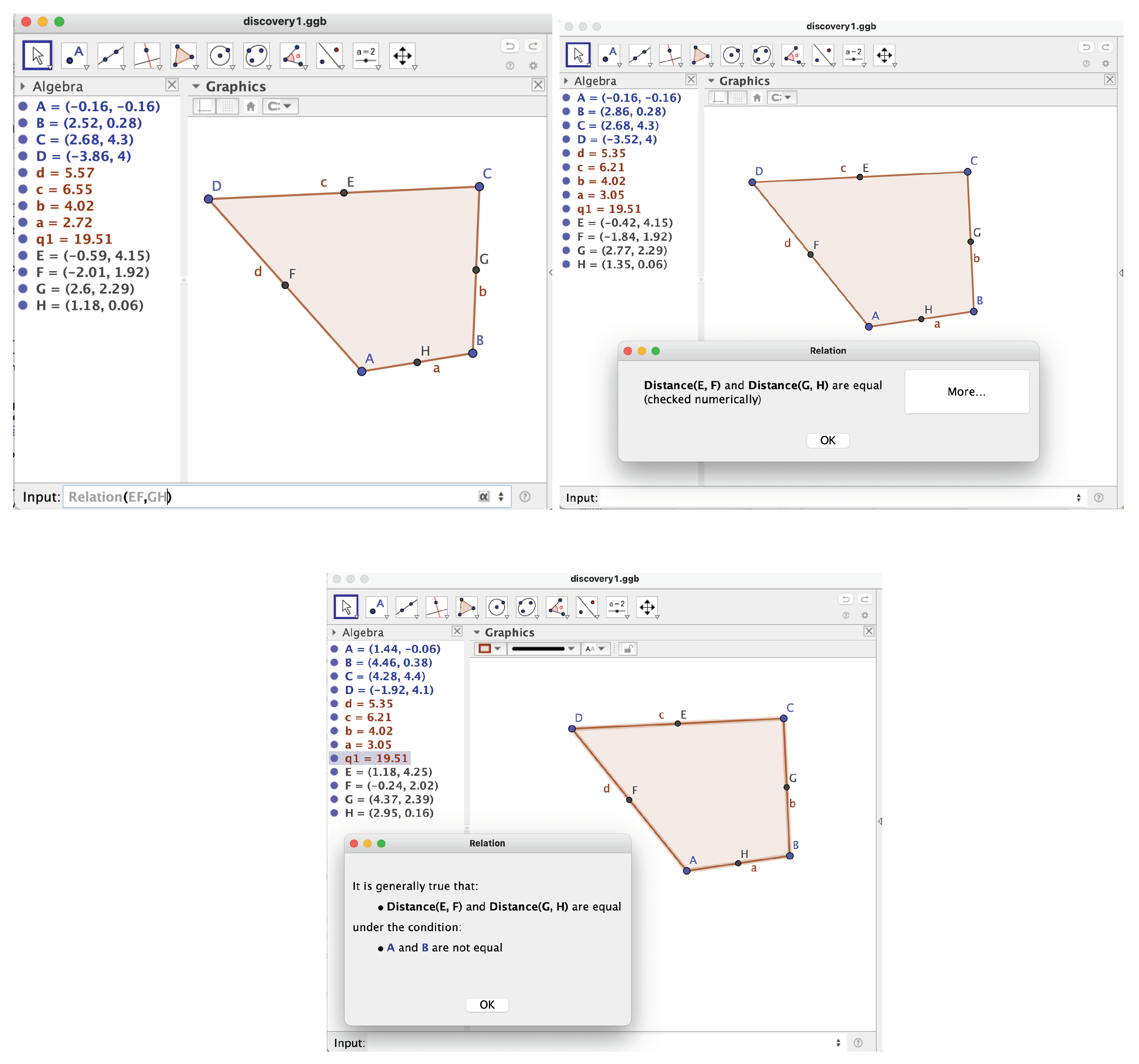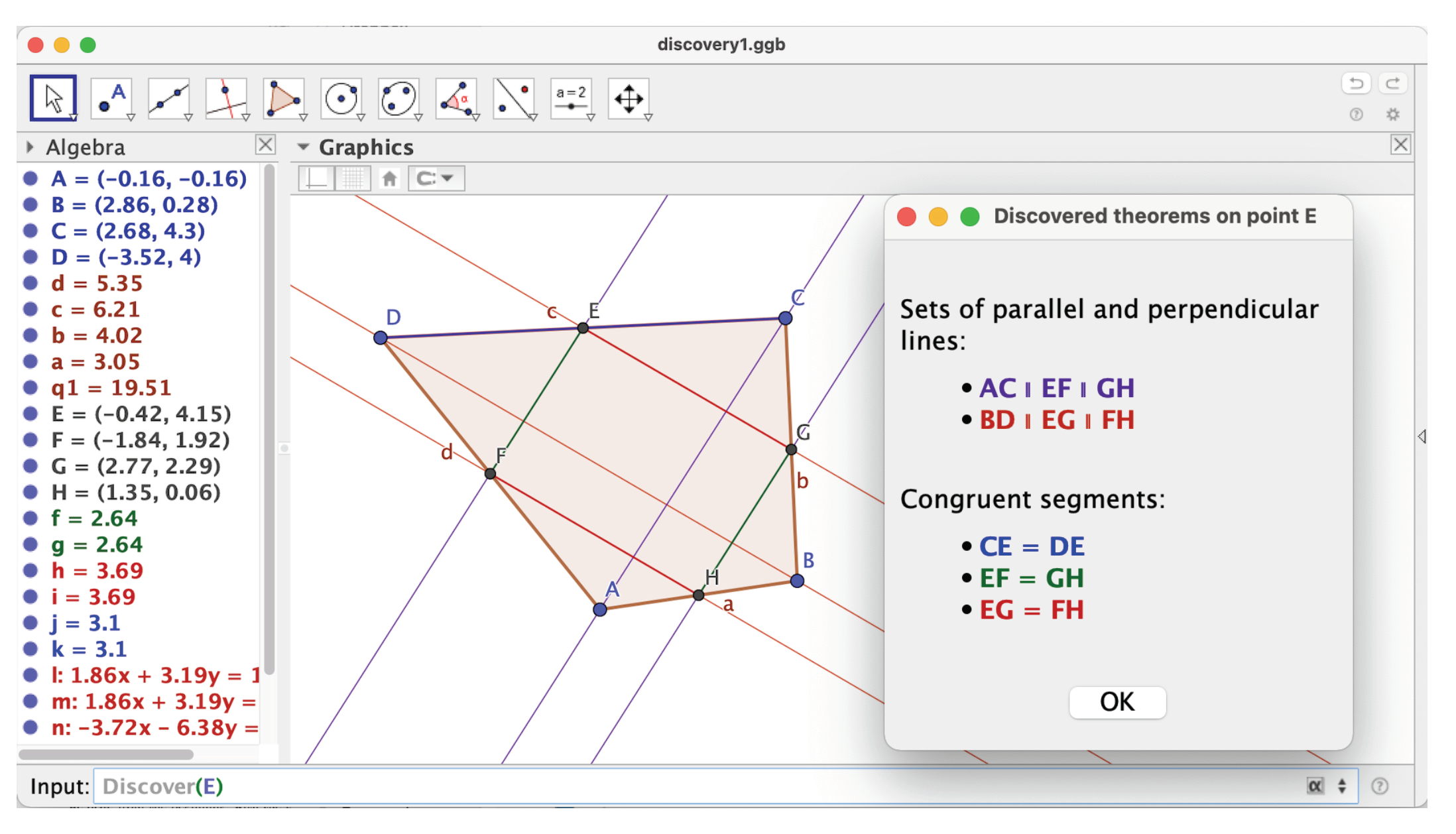In Figure 3 the four vertices of the quadrilateral are free and nothing else, since they determine the midpoints of the sides. 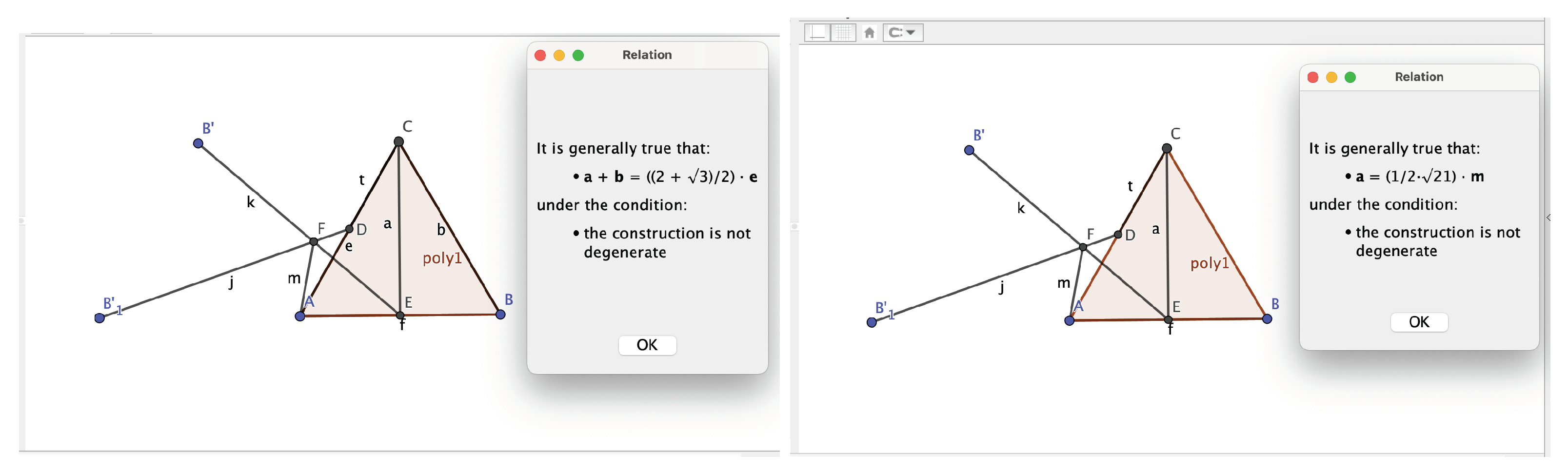In Figure 4, the basic element is an equilateral triangle $A,B,C$, as the other points are clearly depending on this initial data. However, an equilateral triangle is also finitely determined once two vertices are fixed. So, say, here there are only two vertices that actually rule the whole construction, because having a finite number of possible positions for the third vertex can be considered as being determined, anyway. Finally, Figure 7 exemplifies a new situation: the right triangle can be considered as having at least two free vertices $A,B$; and once $A,B$ are fixed, then vertex C is semi-free, as there is an infinite number of possible positions for one of its coordinates (along the circle with diameter $AB$).

Now, the algebraic translation of this concept of “freedom” has to do, first, with the consideration of the coordinates of the points as variables in the polynomial ring describing the geometric statement. The counterpart for the idea of free or semi-free point is, then, the concept of a set of independent variables with respect to an ideal: a set of variables such that there is no polynomial just on these variables in the given ideal. That is, a set of variables such that the given ideal does not include any polynomial constraint among them; namely, they are free. Algorithmically, we are talking about variables such that the elimination of the remaining variables in the ideal yields the zero ideal. Finally, the fact that such free variables “rule” the construction can be thought of as referring to a set of variables so that the remaining ones are finitely determined by the free ones: a maximal set of independent variables.

Unfortunately this condition does not necessarily imply that the cardinal of this maximal set is also maximum among the possible collections of sets of independent variables; i.e., it can be less than the Krull dimension (also known as Hilbert dimension) of the given ideal. For example, consider the ideal $IK[u,v]=〈u·v〉$, where both $\left\{u\right\}$ and $\left\{v\right\}$ are maximal and maximum-size sets of independent variables; and, if $IK[u,v,w]=〈u·v,u·w〉$, then both $\left\{u\right\}$ and $\{v,w\}$ are maximal sets of independent variables, but only the second has cardinality equal to the dimension of I.

This example might look artificial and, indeed, when dealing with geometric statements, it is often assumed in most cases that the ‘intuitively’ maximal set of independent variables is maximum-size, but there are examples in which this is not the case. See Example 2 in ([12], p. 72): the number of coordinates of free points in the chosen geometric construction is 5, but the Hilbert dimension of H is 6; or Example 7 in the Reference [20], about Euler’s formula concerning the distance between the centers and the radii of the inner and outer circles of a triangle with vertices $(-1,0),(1,0),\left(u\right[1],u[2\left]\right)$. Here the ‘intuitive’ dimension of the hypotheses variety should be 2 (the coordinates of the only free vertex of the triangle), but applying the algebraic definition it turns out to be three, unless it is explicitly added to the hypotheses the (obvious) fact that $\left(u\right[1],u[2\left]\right)$ should not lie in the x-axis. This quite common problem—related to the a priori control and detail of all geometric degeneracies—is already considered in the basic Reference [7], mentioning, in particular (cf. page 43), that in many occasions it is not trivial to intuitively prevent, by adding some extra conditions to the hypotheses ideal, the appearance of unwanted situations.

To deal with this complicated context, the current algorithm implemented in GeoGebra automatically associates—following the construction steps—a maximal set of algebraically independent variables to the hypotheses ideal H and considers as ‘degenerate’ those irreducible components of $V\left(H\right)$ where these variables do not remain independent but constrained by some relations. Then, as already defined above, it declares a statement to be generally true (respectively, generally false) iff it is true (false) over all the non-degenerate components.

We will provide further details about this protocol in the next section, but let us remark here that there is a potentially sharper concept of degeneracy, including, besides the components where the chosen algebraically independent variables fail to be independent, those components where these variables remain independent but the dimension of the component is strictly greater than the cardinal of the set of selected variables. This is something geometrically ‘strange’, as it means that the chosen set of variables does not control the construction and there are some ‘unknown’ free points. Following [7], Remark 2, page 47, we will not deal with this notion of degeneracy, considering it irrelevant in practice.

6. A Proposal to Avoid Working with Degeneracy Conditions

Let us fix notation as follows: let us consider K and L to be fields, with L an algebraically closed extension on K (for instance $L=\mathit{C}$ and $K=\mathit{Q}$), and an algebraically translated statement $\{H\Rightarrow T\}$. Let be $H=〈h_1,\dots ,h_r〉$ and $T=〈f〉$ the hypotheses and thesis ideals in the polynomial ring $K\left[X\right]$, where the variables $X=\{x_1,\dots ,x_n\}$ refer to the symbolic coordinates involved in the algebraic description of the hypotheses in $K^n$. Furthermore, take the algebraic variety $V\left(H\right)$ (respectively, $V\left(T\right)$) in the affine space $L^n$ defined over K. Next, fix—following a geometric intuition or through the steps of the geometric construction in the Dynamic Geometry program—a maximal set $Y=\{x_1,\dots ,x_d\}$ of independent variables for the hypotheses ideal H and denote by $Z=\{x_{d+1},\dots ,x_n\}$ the remaining variables.

Definition 1.

We say that a primary component of H, or an irreducible component of $V\left(H\right)$, are non-degenerate iff Y remains independent over the primary component, that is, if there is no polynomial in the Y variables that vanishes over all the corresponding irreducible component.

Remark 1.

Notice that the current definition is similar to the one in [12], but now we are not requiring the dimension of H to be equal to the cardinal of the set of variables, a quite small, but useful in practice, advantage. Moreover, following the consideration in the last paragraph of the previous section, we assume, for the rest of the paper, that non-degenerate components are of dimension d, although d does not have to be the dimension of H.

Now, let us collect different algorithmic criteria for generally true or false statements.

Proposition 1.

The statement $\{H\Rightarrow T\}$ is generally true if and only if

$$〈h_1,\dots ,h_r,f·t-1〉K[X,t]\cap K\left[Y\right]\ne 〈0〉.$$

This result follows from the proof of the first statement in Theorem 1 in [15], bearing in mind that in the proof of that particular item it is not required that Y is of maximum size, with $d=dim\left(H\right)$. On the other hand, following carefully the proof of the second statement in the same Theorem 1, we have the following proposition.

Proposition 2.

The statement $\{H\Rightarrow T\}$ is generally false if

$$〈h_1,\dots ,h_r,f〉K\left[X\right]\cap K\left[Y\right]\ne 〈0〉.$$

Further, adding the condition $dim\left(H\right)=d$, this inequation holds if the statement is generally false.

Definition 2.

Statements that are neither generally true nor generally false are called “true on parts, false on parts” or “true on components”, see [15,16].

These results point out the interest of addressing two further issues:

• How to fully verify the generally false case when $dim\left(H\right)\ne d$? See Example 2 in [15], for a situation where the zero elimination requirement derived from Proposition 2 is necessary but not sufficient for being not generally false.
• How to discriminate non-degenerate components where the thesis holds from those where the thesis fails, in the “true on components” case? This is usually a source of geometric insight, as it shows further restrictions that have to be added for a certain statement to be always true, usually related to the lack of precision of the algebraic translation (e.g., not declaring if the vertex C of an equilateral triangle $A(0,0),B(1,0),C(x,y)$ stands up or down the x-axis, see Example 1 in [15]).

Of course, an immediate solution could be to compute the primary decomposition of H and, then, for each component, to verify if it is, or not, non-degenerate, by eliminating all variables except Y; by definition, the output should be zero iff the component is non-degenerate. Then, over each non-degenerate component, as they are of dimension d, by our assumption—see Definition 1—we could fully apply the criterion expressed in the above propositions.

However, obtaining a complete primary decomposition is usually quite challenging, over a personal computer, through a standard computer algebra program. A much more practical alternative could be the following proposal:

(1)

Isolating the collection of non-degenerate components of H by means of saturation, see Proposition 3 below, and then applying the criteria from the above Propositions.

(2)

Working directly in a zero-dimensional context (as in [16] but without having to compute zero-divisors), extending ideal H to the ring $K\left(Y\right)\left[Z\right]$, i.e., including the selected free variables as elements of the coefficient field.

Let us recall the notion of saturation:

Proposition 3

([21], Prop. 4.9). If S is a multiplicatively closed subset of a ring A and I is a decomposable ideal of A, with a minimal primary decomposition $I=\cap Q_i,i=1\dots n$, then $S^{-1}I$ decomposes with a minimal primary decomposition as $\cap S^{-1}{Q}_i,i=1\dots m$, where $Q_i,i=1\dots m$ denote those primary components such that the associated prime ideals do not meet S. Its contraction (the contraction of the “extension of $=S^{-1}I=S\left(I\right)$”, also called saturation of I) has also as primary minimal decomposition the intersection of $Q_i,i=1\dots m$.

Thus, to address the first item of our proposal, we will consider S as the polynomial ring in the Y variables and thus, computing the saturation we can directly obtain the full collection of non-degenerate components without performing a primary decomposition, thus facilitating the verification of the truth or falsity of the proposition just over the non-degenerate cases (or checking the ‘true on non-degenerate parts’ case). This can be done as follows:

Proposition 4.

Let $H=〈h_1,\dots ,h_r〉$ be an ideal in $K\left[X\right]$. Let $\{g_1,\dots ,g_s\}$ be a Gröbner basis of $〈h_1,\dots ,h_r〉K\left(Y\right)\left[Z\right]$ with respect to any monomial ordering in the variables Z (and coefficients in $K\left(Y\right)$). Where, without loss of generality, $g_i\in K\left[X\right]$, $1\le i\le s$. Let $a_i\left(Y\right)z^{m_i}$ be the leading term of each $g_i$ with respect to the chosen monomial ordering. Furthermore, write $b=a_1\dots a_s$. Then:

$$H^{ec}=〈h_1,\dots ,h_r〉K\left(Y\right)\left[Z\right]\cap K\left[X\right]=〈g_1,\dots ,g_s〉:{\left(b\right)}^{\infty }$$

$$=〈g_1,\dots ,g_s,b·t-1〉K[X,t]\cap K\left[X\right].$$

Proof. 

The last equality is a standard result on saturating an ideal with respect to a polynomial. If $h\in 〈g_1,\dots ,g_s〉:{\left(b\right)}^{\infty }$. Then, for sufficiently large k, $h·b^k\in 〈g_1,\dots ,g_s〉K\left[X\right]$. So, $h·b^k\in 〈g_1,\dots ,g_s〉K\left(Y\right)\left[Z\right]$. But, since $b\in K\left(Y\right)$, $h\in 〈g_1,\dots ,g_s〉K\left(Y\right)\left[Z\right]=H^e$ and $h\in H^{ec}$.

Consider now $h\in H^{ec}$. Then $h\in 〈g_1,\dots ,g_s〉K\left(Y\right)\left[Z\right]$. Since $g_1,\dots ,g_s$ is a Gröbner basis of $H^e$, we can perform the division algorithm of h and $g_1,\dots ,g_s$ (over $K\left(Y\right)\left[Z\right]$) with respect to the monomial ordering. Since the leading coefficient of $g_i$ is a factor of b, we can write:

$$h=g_1·\frac{q_1}{b^k}+\dots +g_s·\frac{q_s}{b^k}$$

with $q_1,\dots ,q_s\in K\left[X\right]$ and a suitable k-th power of b. From this equation

$$h·b^k\in 〈g_1,\dots ,g_s〉K\left[X\right]$$

and

$$h\in 〈g_1,\dots ,g_s〉:{\left(b\right)}^{\infty }.$$

   □

As a more detailed alternative, we can consider the proposal from item (2) above, working directly with the zero-dimensional case. That is, we can extend ideal H to the polynomial ring $K\left(Y\right)\left[Z\right]$ and, as remarked in Proposition 3, we will get only the extension of the components of H such that the Y-variables are free, that is, the non-degenerate. We can perform a primary decomposition of the extended ideal much more simply than for the initial ideal $HK\left[Y\right]\left[Z\right]$, since there are less variables and it is a dimension zero ideal. Now we can decide quite simply about the truth or falsity of the statement over each non-degenerate component as follows:

Proposition 5.

Let $S^{-1}Q$ a component of $HK\left(Y\right)\left[Z\right]$, the extension of a non-degenerate component Q of $HK[Y,Z]=HK\left[X\right]$. Let $〈g_1,\dots ,g_s〉$ a base of $S^{-1}Q$, where the elements $\{g_1,\dots ,g_s\}$ are chosen, clearing denominators, from $K[Y,Z]$. Then the statement $\{Q\Rightarrow T\}$ is true iff

$$〈g_1,\dots ,g_s,f·t-1〉K\left(Y\right)[Z,t]=〈1〉.$$

And the statement $\{Q\Rightarrow T\}$ is false iff

$$〈g_1,\dots ,g_s,f〉K\left(Y\right)\left[Z\right]=〈1〉.$$

Remark that, over a single, irreducible, non-degenerate component, the idea of generally true or generally false is actually the truth or falsity of the statement over the whole component.

Proof. 

Let us recall that $\{g_1,\dots ,g_s\}$ are also elements of Q, since $S\left(Q\right)=Q$, ([21], Prop. 4.8). Now, suppose that $〈g_1,\dots ,g_s,f·t-1〉K\left(Y\right)[Z,t]=〈1〉$. Then, clearing denominators, we will find a non-zero polynomial in Y in $〈g_1,\dots ,g_s,f·t-1〉K\left[Y\right][Z,t]$, that is, over the ring $K[X,t]$. Now, substituting $t=1/f$ and clearing again denominators, we get that a power of f times a polynomial in Y belongs to Q. Since the polynomial in Y cannot be in Q and Q is primary, it follows that a power of the thesis f must be in Q, so $f=0$ over all $V\left(Q\right)$. Conversely, if f vanishes over of $V\left(Q\right)$, a power of f must be in Q, thus $(Q+〈f·t-1〉)K\left[Y\right][Z,t]$ must contain 1, and the same applies ‘a fortiori’ to $〈g_1,\dots ,g_s,f·t-1〉K\left(Y\right)[Z,t]$.

A similar argument proves the second statement. If $1\in 〈g_1,\dots ,g_s,f〉K\left(Y\right)\left[Z\right]$, then there is a non-zero polynomial in Y that is in $〈g_1,\dots ,g_s,f〉K\left[Y\right]\left[Z\right]$, so the vanishing of the thesis over $V\left(Q\right)$ is restricted to the subset of this component where the polynomial in Y vanishes too. As Q is non-degenerate and Y are free over Q, it follows that this subset where the thesis holds is a proper, closed subset of $V\left(Q\right)$. Conversely, if the thesis $f=0$ does not hold over all $V\left(Q\right)$, by the previous Proposition 2, since $dim\left(Q\right)=cardinal\left(Y\right)$, $(Q+〈f〉)K\left[Y\right]\left[Z\right]\cap K\left[Y\right]$ is not zero, thus it has some non-zero polynomial in $K\left[Y\right]$. It follows that this ideal $(Q+〈f〉)K\left(Y\right)\left[Z\right]=〈1〉$.    □

Corollary 1.

Notice that, as a consequence of this proposition, $\{H\Rightarrow T\}$ is generally true if and only if

$$〈h_1,\dots ,h_r,f·t-1〉K\left(Y\right)[Z,t]=〈1〉.$$

Likewise, it is generally false iff

$$〈h_1,\dots ,h_r,f〉K\left(Y\right)\left[Z\right]=〈1〉.$$

Proof. 

In fact, if the statement is generally true, then it is generally true over each component Q of $HK[Y,Z]=HK\left[X\right]$, thus 1 is a combination of elements in $(S^{-1}Q+〈f·t-1〉)$$K\left(Y\right)[Z,t]$. Multiplying all these expressions, for all such Q’s, we get 1 in $(H+〈f·t-1〉)$$K\left(Y\right)[Z,t]$. Conversely, if $1\in (H+〈f·t-1〉)K\left(Y\right)[Z,t]$, then ‘a fortiori’ 1 belongs to every $(S^{-1}Q+〈f·t-1〉)K\left(Y\right)[Z,t]$, and thus the statement is generally true. A similar argument applies to the generally false case.    □

In conclusion, our proposal to deal with degeneracy conditions (rather: to avoid them in an automatic way) could be summarized as follows.

• Choose—from the geometric construction—a meaningful maximal set of independent variables Y. Verify they are actually maximally independent from the algebraic point of view, using elimination commands.
• Restrict the hypotheses variety to the union of non-degenerate components, by using the saturation $S\left(H\right)$ of the hypotheses ideal with respect to S, the polynomial ring in the Y variables.
• Use the elimination commands, as in Proposition 1 and 2, to test the general truth or falsity of the statement over $S\left(H\right)$; or use the Corollary over $S^{-1}H$.
• If the output is ‘true on some, false on some’ non-degenerate components, perform a primary decomposition of $S^{-1}HK\left(Y\right)\left[Z\right]$. Use Proposition 5 to analyze individually each component, as this proposition shows that the result is valid over the corresponding components in $HK[Y,Z]$.

7. An Example

Let us exemplify the use and difficulties of these concepts on a simple, yet illustrative, situation.

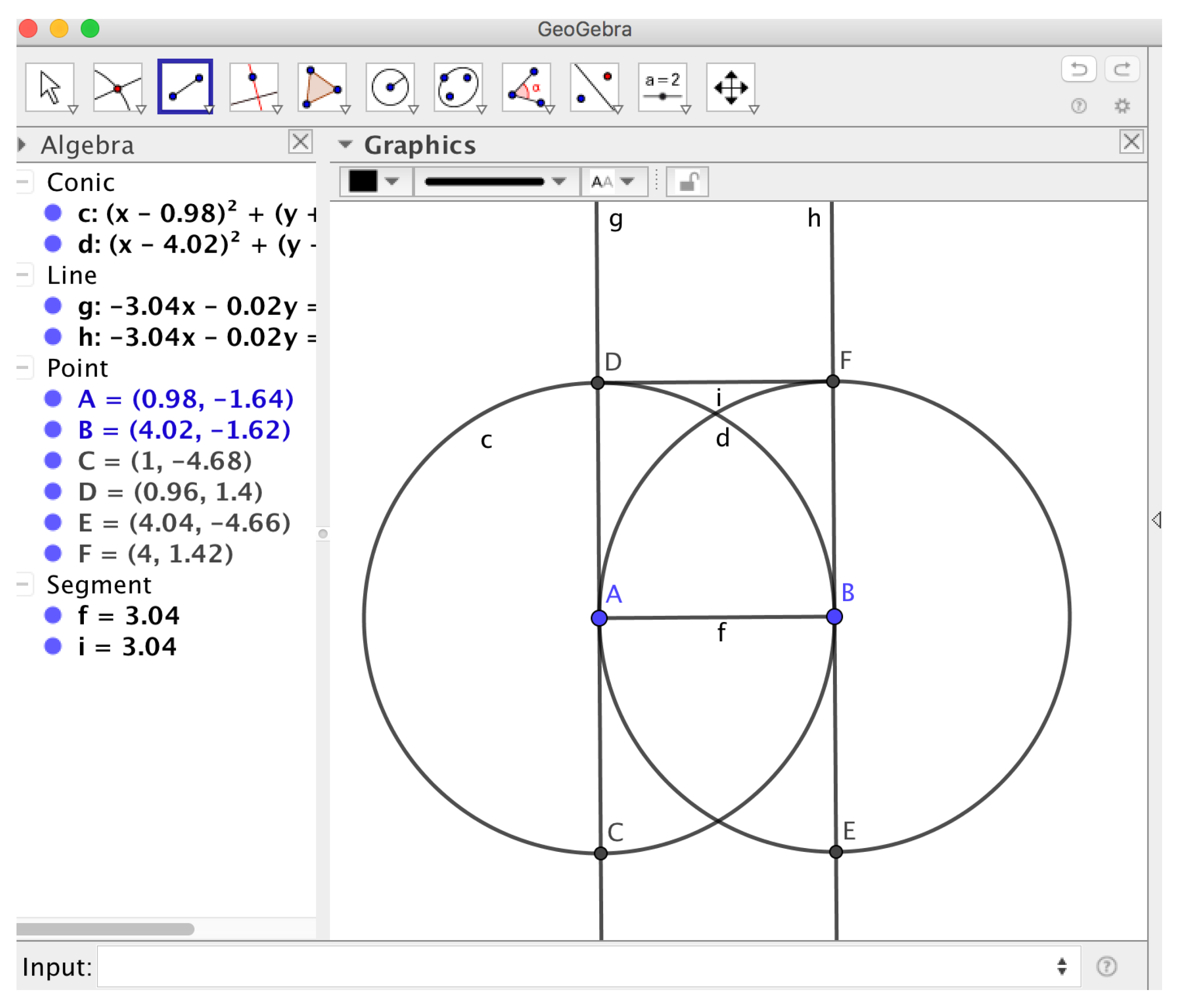
Example 1.

We consider two free points $A,B$. We build circles c (centered at A and passing through B) and d (centered at B and passing through A). The lines $g,h$, through $A,B$ (respectively) are built perpendicular to segment $AB$. Let D and F be the intersection of g with c and of h with $d,$ respectively. Thesis: $DF$ is parallel to $AB$. See Figure 8.

A possible algebraic translation of these hypotheses and thesis could start assigning coordinates $A(a1,a2),B(b1,b2),D(x,y),F(u,v)$ and the corresponding equations

$$c:={(x-a1)}^2+{(y-a2)}^2-({(a1-b1)}^2+{(a2-b2)}^2),$$

$$d:={(u-b1)}^2+{(v-b2)}^2-({(a1-b1)}^2+{(a2-b2)}^2),$$

$$g:=(x-a1)·(b1-a1)+(y-a2)·(b2-a2),$$

$$h:=(u-b1)·(b1-a1)+(v-b2)·(b2-a2).$$

Then point D is defined by these two equations

$${(x-a1)}^2+{(y-a2)}^2-({(a1-b1)}^2+{(a2-b2)}^2)=0,$$

$$(x-a1)·(b1-a1)+(y-a2)·(b2-a2)=0$$

and F is defined by these other two

$${(u-b1)}^2+{(v-b2)}^2-({(a1-b1)}^2+{(a2-b2)}^2)=0,$$

$$(u-b1)·(b1-a1)+(v-b2)·(b2-a2)=0,$$

while the thesis is formulated as $(u-x)·(b2-a2)-(v-y)·(b1-a1)=0.$

It seems intuitively clear that the whole construction is ruled by the coordinates of $A,B$, and so the hypotheses ideal H, including the equations describing $c,d,g,h$ plus those describing points $D,F$, should be of Dimension 4, but it turns out its Hilbert dimension is 5. Indeed $\{a1,a2,b1,b2\}$ are independent variables, but there are sets with five independent variables modulo H, such as $\{a1,a2,b1,x,u\}$, that is, with the coordinates of one of the given free point s (e.g., A), then one single variable from B, one from D, one from F. Let us remark that no set with five independent variables can be found including $\{a1,a2,b1,b2\}$, as expected (see previous comment about [7], Remark 2, page 47). Although the direct computation of the primary components of H is quite involved (for example, it did not succeed within a reasonable amount of time and space, using Maple 2021 on our laptops), we can analyze what happens with the five-dimensional components where, say, $\{a1,a2,b1,x,u\}$ are free, as follows.

First, we will consider S as the polynomial ring in the $\{a1,a2,b1,x,u\}$ variables and thus, if we extend ideal H to the polynomial ring $K(a1,a2,b1,x,u)[b2,y,v]$, and perform there a primary decomposition, we will get only the extension of the components of H such that $\{a1,a2,b1,x,u\}$ are free. It turns out that this much simpler computation yields that $S^{-1}H$ is already prime, of dimension zero, and that it contains the polynomial ${(a1-b1)}^2+{(a2-b2)}^2$. It follows that some polynomials in $\{a1,a2,b1,x,u\}$ times ${(a1-b1)}^2+{(a2-b2)}^2$ will belong to the contraction to $K[a1,a2,b1,b2,x,y,u,v]$ of ‘the’ component of H where $\{a1,a2,b1,x,u\}$ are free. Since by construction no polynomial in $\{a1,a2,b1,x,u\}$ can vanish identically on this component, it means that ${(a1-b1)}^2+{(a2-b2)}^2$ must be zero over the component, that is, interpreted geometrically over the reals, that $A=B$ on this component, so it is degenerate in a ‘real’ sense and $\{a1,a2,b1,b2\}$ are not free! A similar output happens with the other different choices of five independent variables.

On the other hand, considering this set $\{x,y,u,v\}$ of variables, we see that they are also free over H, so we might be interested in investigating what happens with the components that do not meet $S=K[x,y,u,v]$. We repeat the above protocol, getting five components such that, over four of them the variables $\{a1,a2,b1,b2\}$ are also free; however, there is also a component verifying $a1-b1=0$, so we might call it degenerate, although only ‘slightly’ degenerate: a four dimensional component, where points $D,F$ are free and the remaining points are determined by them but are constrained by some relation.

Finally, assuming $Y=\{a1,a2,b1,b2\}$ as the variables defining non-degeneracy in this example and applying the test from Propositions 1 and 2 above, we get

• EliminationIdeal(<(x-a1)^2+(y-a2)^2-((a1-b1)^2+(a2-b2)^2),
• (u-b1)^2+(v-b2)^2-((a1-b1)^2+(a2-b2)^2),
• (x-a1)*(b1-a1)+ (y-a2)*(b2-a2),
• (u-b1)*(b1-a1)+(v-b2)*(b2-a2),
•  ((u-x)*(b2-a2) -(v-y)*(b1-a1))*t-1>,{a1,a2,b1,b2});
•                  <0>
•  
• EliminationIdeal(<(x-a1)^2+(y-a2)^2-((a1-b1)^2+(a2-b2)^2),
• (u-b1)^2+(v-b2)^2-((a1-b1)^2+(a2-b2)^2),(
• x-a1)*(b1-a1)+ (y-a2)*(b2-a2),
• (u-b1)*(b1-a1)+(v-b2)*(b2-a2),
•  ((u-x)*(b2-a2) -(v-y)*(b1-a1))>,{a1,a2,b1,b2});
•                  <0>

which means that the statement is not generally true, but we do not know if it is generally false (as here $dim\left(H\right)\ne cardinal\left(Y\right)$).

Now, we can extend the ideal of hypotheses H to the ring $K(a1,a2,b1,b2)[x,y,u,v]$. One possibility is to apply the above protocol but only to the contraction of this extended ideal, by means of saturation, which is quite obvious in this case (saturation involves only operating with $a1-b1$, after computing a simple Gröbner basis with $tdeg(x,y,u,v)$ that just involves this polynomial as leading coefficient). The output is that, over the non-degenerate components, the statement is clearly true on parts and false on parts.

To be more precise, we can show that this extended ideal $H^e$ has four components (immediately computed on a laptop with Maple 2021). Over each component we can perform the contraction of each component to the initial ring $K[a1,a2,b1,b2,x,y,u,v]$; saturation here is practically obvious, since in every case, the correspondent Gröbner basis with $tdeg(x,y,u,v)$ shows constant (in K) leading coefficients. Finally, we can perform the above test over the contracted components, yielding that the statement is true on two of them and false on other two (in this case, suggesting that ${(a1-b1)}^2+{(a2-b2)}^2=0$ is a required extra condition for the truth of the statement on the components where it fails).

Alternatively, we can work directly over on $K(a1,a2,b1,b2)[x,y,u,v]$ and verify if 1 is or not in the elimination of the component ideals plus $〈f·t-1〉$ or $〈f〉$, as in Proposition 5 above. The answer is true, false for the first and fourth components and false, true for the other two, as expected.

We refer the interested reader to https://doi.org/10.5281/zenodo.5179979 (accessed on 13 August 2021) for a MW and PDF files detailing the Maple computations we have described in this section.

8. Conclusions

Dealing with degeneracy conditions is a quite relevant subject in the development of geometric automated reasoning tools, even more relevant when such tools are at the disposition of a great number of potential users, and in very different contexts, such as educational, most of them are far from involving researchers and mathematical experts. We have focused on proposing different ways to avoid the impact of degeneracy conditions by extending the coefficient ring, including the free variables of the hypotheses set as parameters, and exploiting, in different ways, the possibilities of this simplified situation.

Of course this protocol does not avoid the possible occurrence of some unexpected outputs, due to other issues, due, for example, to the need to consider inequations (e.g., for working with distances or with polynomials with only even powers, etc.) or to the the lack of precision of some constraints, when dealing with different roots of a single algebraic equation (and we are geometrically considering only one of them), etc. Yet, we think that our protocol can help, at least, in ‘cleaning’ the path to diminish the possible interpretations and, in any case, to understand the reasons behind some unexpected results, as shown in the example in the last section.