Article

Analytical and Numerical Connections between Fractional Fickian and Intravoxel Incoherent Motion Models of Diffusion MRI

1
Department of Radiology and Imaging Science, Emory University, Atlanta, GA 30322, USA
2
Department of Orthopedics, Emory University, Atlanta, GA 30322, USA
*
Author to whom correspondence should be addressed.
Mathematics 2021, 9(16), 1963; https://doi.org/10.3390/math9161963
Submission received: 1 June 2021 / Revised: 4 August 2021 / Accepted: 9 August 2021 / Published: 17 August 2021
(This article belongs to the Special Issue Fractional Calculus in Magnetic Resonance)

Abstract

:
Impaired tissue perfusion underlies many chronic disease states and aging. Diffusion-weighted imaging (DWI) is a noninvasive MRI technique that has been widely used to characterize tissue perfusion. Parametric models based on DWI measurements can characterize microvascular perfusion modulated by functional and microstructural alterations in the skeletal muscle. The intravoxel incoherent motion (IVIM) model uses a biexponential form to quantify the incoherent motion of water molecules in the microvasculature at low b-values of DWI measurements. The fractional Fickian diffusion (FFD) model is a parsimonious representation of anomalous superdiffusion that uses the stretched exponential form and can be used to quantify the microvascular volume of skeletal muscle. Both models are established measures of perfusion based on DWI, and the prognostic value of model parameters for identifying pathophysiological processes has been studied. Although the mathematical properties of individual models have been previously reported, quantitative connections between IVIM and FFD models have not been examined. This work provides a mathematical framework for obtaining a direct, one-way transformation of the parameters of the stretched exponential model to those of the biexponential model. Numerical simulations are implemented, and the results corroborate analytical results. Additionally, analysis of in vivo DWI measurements in skeletal muscle using both biexponential and stretched exponential models is shown and compared with analytical and numerical models. These results demonstrate the difficulty of model selection based on goodness of fit to experimental data. This analysis provides a framework for better interpreting and harmonizing perfusion parameters from experimental results using these two different models.

1. Introduction

Microvascular perfusion in skeletal muscle is essential for nutrient supply and cellular metabolism [1]. Compromised skeletal muscle perfusion underlies many disease conditions [2,3] and the reduction and loss of mobility with aging [4]. Impaired skeletal muscle perfusion can be related to physical properties such as loss of microvascular function, reduced blood flow, and the rarefaction of microvessels. Diffusion-weighted magnetic resonance imaging (DW-MRI) is a noninvasive measurement that is sensitive to molecular motions in water occurring at different rates within microvasculature and tissue parenchyma, respectively [5]. Thus, the consideration of appropriate signal models and DW-MRI acquisition schemes for quantifying physical properties of these tissue compartments is of particular interest for assessing perfusion in skeletal muscle.
The intravoxel incoherent motion (IVIM) [6] and fractional Fickian diffusion (FFD) models [7] are well-established mathematical representations used to characterize DW-MRI measurements. Compared with the classical single compartmental model which characterizes the random Brownian motion of all tissue water molecules as a monoexponential decay of MRI signal, the IVIM model uses a biexponential representation to differentiate the incoherent motion of intra-vascular blood perfusion and extra-vascular water proton diffusion. The FFD model is a parsimonious representation of anomalous superdiffusion that models the diffusion decay signal as a stretched exponential. In this model, a single diffusion compartment is represented for an exponent value of 1 and superdiffusion is represented when the exponent decreases to values less than 1. This fractional-order model is convenient as it is more robust, with a limited number of diffusion weightings, and more reliable in the presence of noise [8]. However, the relationship between the FFD model parameters and physical tissue parameters is not as straightforward as that of the IVIM model. Comparisons of the biexponential and stretched exponential models have been made extensively in terms of their applications for the diagnosis and grading of disease stages [9,10,11]. The stretched exponential is reported to outperform the biexponential model with a lower estimate variance and higher reproducibility [8,9,10,12]. However, the underlying connection between the two models has not been previously established, making it challenging to select an appropriate model for characterizing perfusion in specific conditions. Furthermore, an analytical framework that could transform the stretched exponential fit parameters to the intuitive picture of the two-compartment IVIM model could provide utility in comparing and interpreting experimental results.
This work establishes an analytical framework for direct comparisons between the biexponential and stretched exponential models. The explicit representation of the equivalent biexponential model parameters is provided in terms of the stretched exponential model for facilitating comparisons. These analytical expressions and numerical analyses are used to compare models under a range of model parameters that are experimentally encountered in the application of DW-MRI to perfusion measurements of skeletal muscle. The analysis of in vivo DW-MRI data from skeletal muscle is presented as they relate to analytic and numerical results.

2. Definitions and Properties

The most commonly implemented DW-MRI sequence is the pulsed gradient spin echo (PGSE) [13]. This sequence applies diffusion-sensitizing gradients before and after a refocusing radiofrequency pulse separated by a fixed diffusion waiting period, where adjustments to gradient strength are used to set the desired level of diffusion sensitization. Thus, hydrogen nuclei exhibiting motions along the direction of the diffusion sensitizing gradients lose phase coherence proportional to the amount of motion. For the classic Stejskal–Tanner pulse sequence [14], the model used to describe the magnitude of signal attenuation can be expressed in terms of the gradient duration (δ), strength (g), and the time interval between gradient pulses (Δ):
y ( g , δ , Δ ) = y 0 e D ( γ g δ ) 2 ( Δ δ 3 ) ,
where y 0 is the equilibrium magnetization in the absence of diffusion sensitizing gradients, D is the apparent diffusion coefficient with units of mm2/s, γ is the gyromagnetic ratio, and Δ   δ [15]. With the majority of clinical MRI scanners using fixed values of δ and Δ, this expression is routinely simplified:
y ( b ) = y 0 e D b ,
where b is the diffusion-weighting value with units of s/mm2. Thus, a common way to adjust diffusion weighting is to vary the gradient amplitude.
The diffusion model has been extended to quantify incoherent motions of blood water protons in the microvascular space. Because the rate of incoherent motions of the blood pool can be orders of magnitude greater than the rate of thermal diffusion of body water, perfusion measurements rely on small values of b, typically sampled in a range between 0 and 200 s/mm2. The most well-known perfusion model—IVIM—extends Equation (2) above by taking a biexponential form [6]. This model allows for the fractional pool size and rate of the more rapidly moving blood pool to be quantified separately from that of the tissue water in the extra-vascular space. A more recent emerging perfusion model—FFD--takes the form of a stretched exponential signal model. This model imposes a fractional time derivative on Fick’s law which allows for the modeling of the non-Gaussian jump length statistics expected from blood perfusion within the multiscale vascular bed [16].

2.1. Biexponential Model

As introduced above, the IVIM model uses a biexponential signal model:
y b e ( b ) = y 0 [ f p e D p b + ( 1 f p ) e D b ] ,
where y b e ( b ) is the MR signal intensity at a particular b value, b is the diffusion-sensitizing factor with units s / mm 2 , y 0 is the equilibrium magnetization when b = 0 , f p is the perfusion fraction ( 0 f p 1 ), D p is the pseudodiffusion coefficient (or perfusion coefficient) with units mm 2 / s , and D is the apparent diffusion coefficient of water molecules in the extra-vascular tissue with units mm 2 / s . The two exponentials in the model correspond to compartments of intra- and extra-vascular tissue that are characterized by the decay rates, D p and D , respectively. Extending the number of compartments with an improved multi-exponential model can account for additional compartments in the vascular tissue, but it is challenged by the increased number of fitting parameters.

2.2. Stretched Exponential Model

The stretched exponential signal model is a parsimonious representation of anomalous superdiffusion, which is a non-Gaussian diffusion that exhibits greater particle spread than would be expected from Gaussian diffusion [17]. This signal model is expressed as a function of the b value as follows:
y s e ( b ) = y 0 e ( ( D s e · b ) α / 2 )
where D s e is the diffusion coefficient in the stretched exponential model with units mm 2 / s , and α is the stretching exponent representing the fractional derivative order [17]. Note that, to exhibit sensitivity to perfusion in a complex and heterogeneous system like skeletal muscle, the stretched exponential model requires the sampling of b so that b · D s e 1 . For diffusion sequence parameters in the range of b · D s e > 1 , this model is interpreted in the context of hindered diffusion which probes a different aspect of the tissue [18]. In the derivation of the FFD model, 0 < α 2 with smaller values of α reflecting an increase in perfusion [16]. In particular, the stretched exponential becomes a monoexponential model when α = 2 . In the remainder of the current work, we use a simplifying step using α ^ = α / 2 where 0 < α ^ 1 .
Although it is not the physical picture of the FFD model, another interpretation of the stretched exponential model is that it represents a sum of exponentials [19,20]. Thus, numerically the biexponential model can be considered as a truncated representation of the stretched exponential model. Compared with the biexponential model, the parsimonious stretched exponential model has one less fitting parameter, leading to an inherently smaller fitting estimate variance [21].

3. Materials and Methods

3.1. Biexponential Representation of the Stretched Exponential Model Parameters

To obtain the biexponential representation of the stretched exponential model, we consider the three biexponential model parameters { f p ,   D p , D } as unknowns, with y 0 being eliminated from Equation (3) by normalizing diffusion weighted images by the b = 0 image. The goal is to solve for these three unknowns given the two stretched exponential parameters { α ^ , D s e } . Three unknowns require three samples from the stretched exponential signal to form a fully determined case. When there are more than three samples, an over-determined case is established, leading to an estimate of biexponential parameter values rather than exact analytical solutions. For both models, b values are sampled either uniformly spaced or non-uniformly spaced.
The stretched exponential model in Equation (4) can be normalized by the equilibrium magnetization at the b = 0 condition, y 0 :
y ˜ s e ( b ) = y ( b ) y 0 = e ( ( D s e · b ) α ^ ) = ( e D s e α ) b α ^
Similarly, the biexponential model in Equation (3) can be normalized to:
y ˜ b e ( b ) = y ( b ) y 0 = f p e D p b + ( 1 f p ) e D b = f p e D p b + f e D b
with f = ( 1 f p ) and b { 0 , 1 , 2 , } . Given the sampling interval ( τ ) of b , D p = D ^ p τ and D = D ^ τ where D ^ p and D ^ are the respective pseudodiffusion coefficient and apparent diffusion coefficient normalized by τ .
Making the substitution η = e D s e α ^ and taking the z-transform of y ˜ s e ( b ) in Equation (5) and that of y ˜ b e ( b ) in Equation (6) leads to:
Y s e ( z ) = b = 0 η b α ^ z b = 1 + η z 1 + η 2 α ^ z 2 + η 3 α ^ z 3 +
and
Y b e ( z ) = f p 1 e D p z 1 + f 1 e D z 1
Expanding and rewriting Equation (8) using ρ 1 = e D p and ρ 2 = e D yields:
Y b e ( z ) = b 0 + b 1 z 1 1 + a 1 z 1 + a 2 z 2
where
b 0 = f p + f = 1 ;   b 1 = ( ρ 1 f + ρ 2 f p ) ;   a 1 = ( ρ 1 + ρ 2 ) ;   and   a 2 = ρ 1 ρ 2 .
Long division to the right-hand-side (RHS) of Equation (9) results in:
Y b e ( z ) = b 0 + ( b 1 b 0 a 1 ) z 1 { b 0 a 2 + a 1 ( b 1 b 0 a 1 ) } z 2 + [ a 1 { b 0 a 2 + a 1 ( b 1 b 0 a 1 ) } a 2 ( b 1 b 0 a 1 ) ] z 3 +
Now the RHS of Equations (11) and (7) are both in the form of the z -term sums. Comparing coefficients of corresponding z-terms of Equations (11) and (7), we obtain:
b 0 = 1 , ( b 1 b 0 a 1 ) = η , { b 0 a 2 + a 1 ( b 1 b 0 a 1 ) } = η 2 α ^ , a 1 { b 0 a 2 + a 1 ( b 1 b 0 a 1 ) } a 2 ( b 1 b 0 a 1 ) = η 3 α ^ ,
The unknowns { b 1 , a 1 , a 2 } in Equation (12) are associated with the biexponential model parameters { f p ,   D p , D } according to Equation (10), and can be solved with a minimum of three stretched exponential model samples { η ,   η 2 α ^ ,   η 3 α ^ } , as displayed in Equation (12). As implied from Equation (12), these analytical expressions based on the z transform require uniform b value sampling.
In the case where three uniformly spaced samples of the stretched exponential model are given, the fully determined case is established. This yields exact solutions to b 1 ,   a 1 , and a 2 and, subsequently, exact analytical solutions to f p ,   D p and D . By simplifying the Equation (12) by back-substituting terms, we obtain:
{ a 2 a 1 η = η 2 α ^ , a 2 η a 1 η 2 α = η 3 α ^ ,
which can be written in matrix form as:
[ η 1 η 2 α η ] [ a 1 a 2 ] = [ η 2 α ^ η 3 α ^ ]
The fully determined 2 × 2 matrix in Equation (14) allows for analytical solutions to a 1 , a 2 , using ( b 1 b 0 a 1 ) = η in Equation (12), that of b 1 :
a 1 = η 3 α ^ η η 2 α ^ η 2 α η 2 ;   a 2 = η η 3 α ^ η 2 α ^ + 1 η 2 α η 2 ;   b 1 = η ( 2 η 2 α ^ η 2 ) η 3 α ^ η 2 α ^ η 2 .
Then, a 1 and a 2 from Equation (15) are substituted in Equation (10) to solve for ρ 1 and ρ 2 :
ρ 1 , 2 = a 1 ± a 1 2 4 a 2 2
For the IVIM model, ρ 1 = e D p , ρ 2 = e D , and the pseudo-diffusion coefficient D p is larger than the diffusion coefficient D , thus, ρ 1 < ρ 2 . We obtain:
{ ρ 1 = a 1 a 1 2 4 a 2 2 , ρ 2 = a 1 + a 1 2 4 a 2 2 ,
The values f p and f can be determined based on Equation (10) where:
{ b 0 = 1 = f p + f , b 1 = ( ρ 1 f + ρ 2 f p ) .
This appears as follows in matrix form:
[ 1 1 ρ 2 ρ 1 ] [ f p f ] = [ 1 b 1 ]
with the following solutions to f p and f :
{ f p = b 1 + ρ 1 ρ 1 ρ 2 , f = 1 f p = b 1 + ρ 2 ρ 1 ρ 2 .
Our goal is to calculate the biexponential model parameters { f p , D p , D } based on the known stretched exponential parameters { α , ^ D s e } . Up until this point, the following relationships between stretched and biexponential model parameters have been obtained:
{ f p = b 1 + ρ 1 ρ 1 ρ 2 e D p = ρ 1 = a 1 a 1 2 4 a 2 2 e D = ρ 2 = a 1 + a 1 2 4 a 2 2
Combining solutions to b 1 , ρ 1 , ρ 2 , a 1 and a 2 into Equation (21), produces analytical expressions for { f p , D p , D } in the form of η which is defined above as η = e D s e α ^ .
D p = ln { η 3 α ^ η η 2 α ^ η 2 * 3 α ^ + η η 3 α ^ ( 4 η 2 6 η 2 α ^ ) + 4 η 3 * 2 α ^ 3 η 2 η 2 α ^ + 1 2 ( η 2 α ^ η 2 ) } , D = ln { η 3 α ^ η η 2 α ^ + η 2 * 3 α ^ + η η 3 α ^ ( 4 η 2 6 η 2 α ^ ) + 4 η 3 * 2 α ^ 3 η 2 η 2 α ^ + 1 2 ( η 2 α ^ η 2 ) } , f p = 0.5 { 1 + η 3 α ^ η ( 3 η 2 α ^ 2 η 2 ) η 2 * 3 α ^ + η η 3 α ^ ( 4 η 2 6 η 2 α ^ ) + 4 η 3 * 2 α ^ 3 η 2 η 2 α ^ + 1 } , f = 1 f p = 0.5 { 1 η 3 α ^ η ( 3 η 2 α ^ 2 η 2 ) η 2 * 3 α ^ + η η 3 α ^ ( 4 η 2 6 η 2 α ^ ) + 4 η 3 * 2 α ^ 3 η 2 η 2 α ^ + 1 } .

3.2. Biexponential Estimates of the Stretched Exponential Model Parameters

In practice, DW-MRI images are acquired using several non-uniformly spaced b values (i.e., >3) for estimating perfusion and diffusion properties. This sampling scheme results in an over-determined matrix for solving a 1 , a 2 , b 1 , and subsequently f p ,   D p and D . Specifically, the matrix in the left-hand side of Equation (14) becomes:
[ η b 1 α ^ η b 0 α ^ η b 2 α ^ η b 1 α ^ η b k 1 α ^ η b k 2 α ^ ] [ a 1 a 2 ] = [ η b 2 α ^ η b 3 α ^ η b k α ^ ]
where b k = k for k { 0 , 1 , 2 , } in a generalized form. Equation (23) can be written as Π a = p , where Π is a ( k 1 ) × 2 tall matrix, a is a column vector consists of a 1 and a 2 , and p is a column vector with ( k 1 ) elements. The method of least squares (LS) [22] to obtain a ^ = ( Π T Π ) 1 Π T p , as estimates of a . The analytical expression for the biexponential fit estimates that f p ^ , D ^ p and D ^ , can be computed in a manner similar to subsequent steps following Equation (15) in Section 3.1, though the expressions may not be as tractable as Equation (22), obtained for the fully determined case.

3.2.1. Error Analysis

Mean squared error (MSE) in the biexponential modeling of the stretched exponential process can be expressed as:
E { e 2 ( b ) } = E { y ˜ s e ( b ) y ˜ b e ( b ) } 2
where e ( b ) is the model representation error, and E is the expectation operator. Expanding the right-hand-side of (24) leads to:
E { e 2 ( b ) } = E { y ˜ s e 2 ( b ) + y ˜ b e 2 ( b ) 2 y ˜ s e ( b ) y ˜ b e ( b ) } .
Substituting respective values of y ˜ s e ( b ) and y ˜ b e ( b ) from Equations (5) and (6) into (25) leads to:
E { e 2 ( b ) } = E { η 2 b α ^   } + E { ( f p ρ 1 b + f ρ 2 b ) 2 } 2 E { η b α ^   ( f p ρ 1 b + f ρ 2 b ) }
with η = e D s e α ^ , and ρ 1 = e D p and ρ 2 = e D . Equation (26) shows that MSE is a function of the stretching exponent α ^ . MSE is zero when f p ρ 1 b = η b α ^ and f ρ 2 b = 0 , or vice versa, implying α ^ = 0 ,   1. The stretched exponential becomes a constant value signal for α ^ = 0 , and a mono-exponential signal for α ^ = 1 .

3.2.2. Error Analysis in the Presence of Noise

In the presence of the independent and identically distributed additive Gaussian noise v ( b ) of zero mean and σ 2 variance, Equation (26) becomes:
E { e 2 ( b ) } = E { η 2 b α ^   } + E { ( f p ρ 1 b + f ρ 2 b ) 2 } 2 E { η b α ^   ( f p ρ 1 b + f ρ 2 b ) } + σ 2
with E { v 2 ( b ) } = σ 2 . MSE is reduced to σ 2 when α ^ = 0 ,   1. This will serve as the lower bound for the MSE. For 0 < α ^ < 1 , MSE will be larger than σ 2 .

3.2.3. Model Simulations and Cross-Model Error Analysis

To compare the analytical and numerical solutions derived in Section 3.1 and Section 3.2, forward simulation of stretched exponential signal decays are generated and fitted using the biexponential expressions. Noise is not considered for either the forward or estimated model. All simulations are implemented with custom-written MATLAB (MathWorks 2019b, Natick, MA, USA) scripts.
The z-plane analysis is performed as a way of examining the relationship between biexponential parameters to the stretched exponential signal model. A simulation is implemented for the fully determined case when b = 0, 1, 2, and 3 and D s e = 1 / b m a x . This utilizes the analytical expressions relating the biexponential model parameters to that of the stretched exponential, based on the fully determined case. These b values, although not representative of values used experimentally, in combination with the selection of D s e = 1 / b m a x , reflect the typical scaling used in experimental settings D s e · b m a x = 1 . With this analysis, analytical expressions obtained for biexponential model parameters { f p ,   f ,   D p ,   D } in Equation (22) can be jointly visualized as a function of stretched exponential parameters { α ^ ,   D s e } , using the so-called three-dimensional z-plane plot. According to Equation (8), the biexponential model corresponds to two poles, ρ 1 = e D p and ρ 2 = e D with their respective damping amplitudes f p and f . In the three-dimensional z plane plot, the two in-plane axes refer to the real and imaginary parts of a pole, and the vertical axis refers to the corresponding damping amplitude. When D s e is fixed, the trajectory of a pole is directed by the stretched exponential model parameter α ^ .
Simulations for the over-determined case compare estimated biexponential parameters with their corresponding analytical solutions for 0 < α ^ 1 , at a fixed b m a x and D s e = 1 b m a x . Sampling schemes of b values at various sample spacings were examined and compared with the analytical solutions to biexponential model parameters. Analytical expressions are computed and shown for two limiting cases: (1) D s e = 1 / 3 and (2) D s e = 1 / 400 .
The divergence between the simulated signal y s e ( b ) and estimated signal y ^ s e ( b ) of the stretched exponential model is quantified using mean-squared-error (MSE) analysis. Given uniformly spaced b values and D s e = 1 b m a x , MSE is computed as a function of α ^ , defined as ε ( α ^ ) = 1 N n = 1 N ( y s e ( b n ) y ^ s e ( b n ) ) 2 , where N is the number of b values, and signal values y s e ( b n ) and y ^ s e ( b n ) are modulated by the argument α ^ (refer to equation (5)). Additionally, the autocorrelation of the error sequence ε ( α ^ , m ) = 1 N r e e ( m ) , is computed as is a function of α ^ and delay m , where m is the b-value lag, and r e e ( m ) represents the autocorrelation function of the residual e ( b n ) = y s e ( b n ) y ^ s e ( b n ) .

3.3. In Vivo MRI Acquisition

To illustrate the analytical and numerical analysis of the IVIM and FFD models, we compared model fit parameters from DW-MRI data from a single healthy volunteer. Data were obtained as part of the Genetic and Epigenetic Signatures of Translational Aging Laboratory Testing (GESTALT) study under approval by IRB through the National Institute of Environmental Health Sciences.
The exercise protocol was described in existing publications [16,23]. Briefly, DW-MRI was obtained before and immediately after performing an in-magnet knee extension exercise with an MR-compatible ergometer (Quadspect; Ergospect, Innsbruck, Austria) at a frequency of 45 repetitions per minute for 2.5 min using the left leg. The pedal resistance was fixed at 0.4 bar.
The participant was imaged using a 3T Achieva MRI scanner (Phillips Healthcare, Best, Netherlands) using a two-channel SENSE flexible coil positioned at the mid-thigh level. The DWI measurements were acquired using a single transverse slice of thickness 22 mm at mid-thigh, using a spin-echo single-shot EPI readout with diffusion sensitization in the slice direction, with triple fat suppression to reduce the effect of fat signal on the measurements. Sequence parameters included TR = 3000 ms, TE = 46 ms, SENSE factor = 2, FOV = 256 × 225 mm, matrix size = 224 × 224, partial Fourier factor = 0.5, diffusion gradient duration δ = 27 ms, diffusion gradient interval Δ = 35 ms, and 14 non-uniformly spaced b values: 0, 3, 7, 10, 15, 20, 25, 30, 40, 50, 70, 100, 200, and 400 s/mm2. DWI acquisition at rest performed 20 signal averages (acquisition time = 16.05 min) in order to increase SNR under low perfusion conditions, while post-exercise acquisition performed 4 signal averages (acquisition time = 3.25 min). All images exhibited SNR > 200, deemed sufficient for robust estimates of parameters [23,24].
Regions of interest (ROI) were selected within the rectus femoris and vastus lateralis, which were part of the active muscle groups during knee extension exercise. ROIs were drawn to exclude blood vessels, fat and fasciae. Pixel-wise fits were performed within each ROI using the biexponential (Equation (6)) and stretched exponential (Equation (5)) models, respectively. The connection between parameters from the two model fits was compared with the simulation results obtained from the overdetermined case described in Section 3.2. Parameter comparisons were made from resting muscle and muscle after exercise, representing a large dynamic range of model parameters observed in vivo.

4. Results

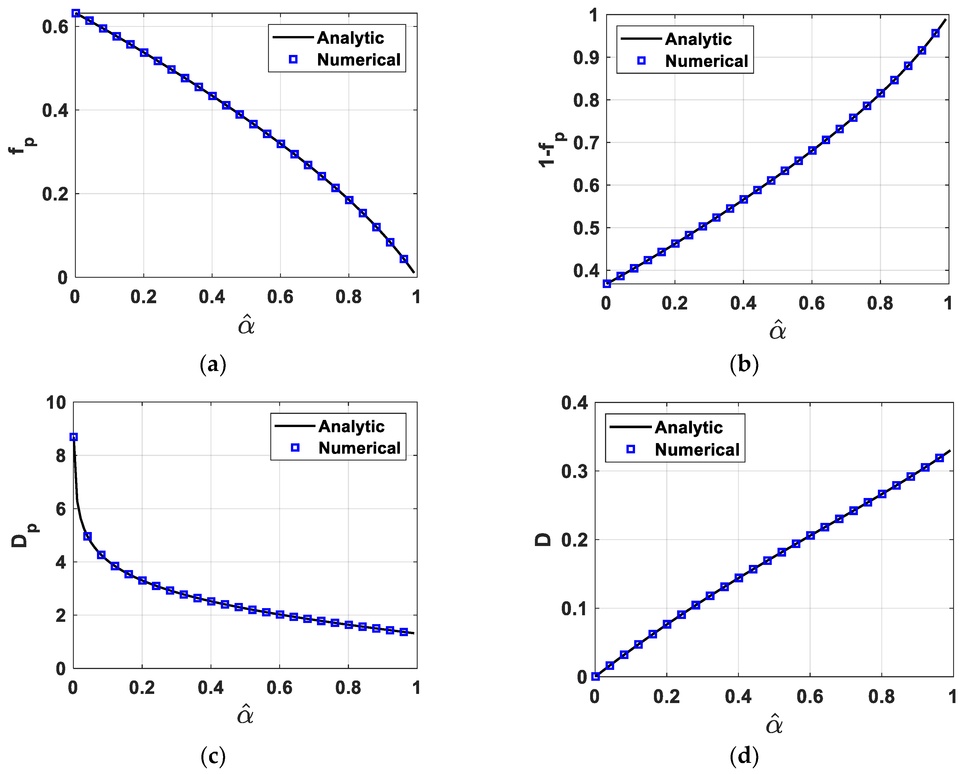
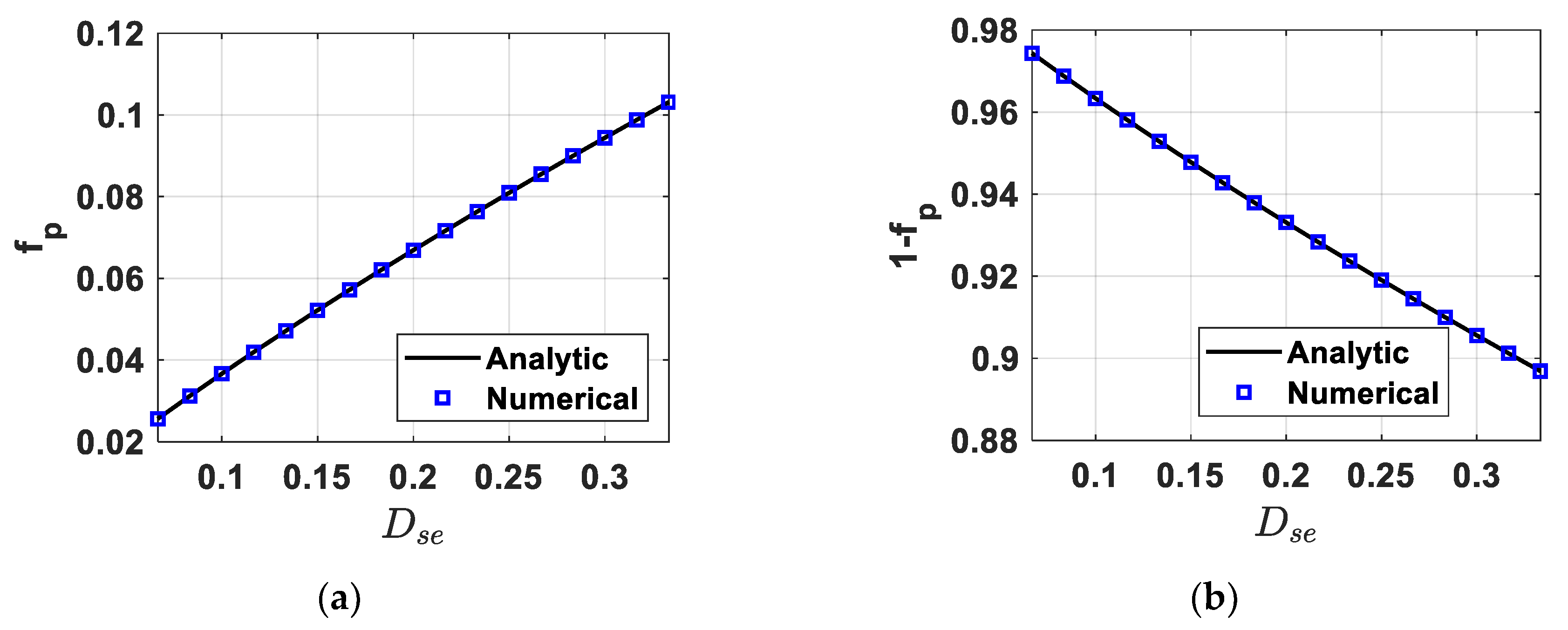
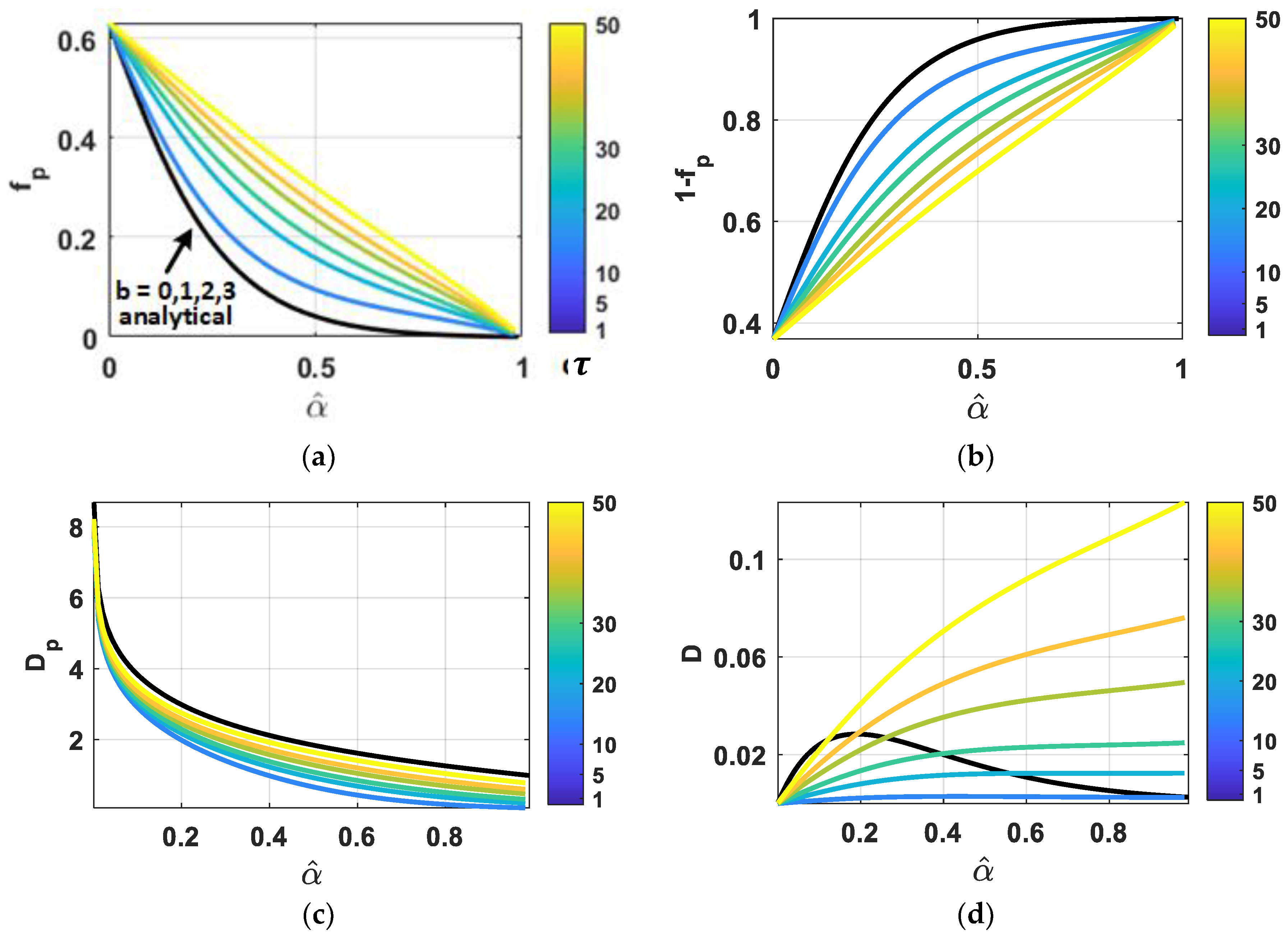
4.1. Fully-Determined Case

Analytical expressions relating the biexponential and stretched exponential model parameters were used to generate Figure 1 and Figure 2, using uniformly spaced b values ( b = 0 , 1, 2, 3). These analytical relationships for the parameters f p ,   D p and D showed excellent correspondence with the numerical solutions derived in Section 3.2 over the range of simulated α ^ and D s e values, respectively.
Figure 3 shows each biexponential model parameter with respect to the bivariant combinations of the stretched exponential model parameters α ^ and D s e . These plots illustrate how biexponential parameters are influenced by the relationship between D s e and b m a x . Specifically, these plots illustrate the relatively more pronounced nonlinear influence of α ^ on biexponential parameters, as D s e · b m a x decreases from 1.
Figure 4 shows the z-plane analysis, which illustrates the pole trajectories and their corresponding damping amplitudes. Trajectories of both poles lie on the real-axis of the z-plane, indicating that the biexponential estimates based on the stretched exponential data reconstruct real exponentials only. Both poles lie within the unit circle, indicating that the biexponential estimates of the stretched exponential model are stable. The trajectories of the two poles do not coincide, implying that the solution space for the biexponential model is localized for estimating the forward model of the stretched exponential model.
In the projection on the z-plane, a pole closer to the unit circle boundary exhibits a slower decay rate that corresponds to a narrower diffusion jump length distribution. The pole closer to the center of the unit circle exhibits a faster decay rate and contributes to the relatively heavy tail in the jump length distribution. As α ^ changes progressively from 0+ to 1, the pole associated with pseudo-diffusion travels from the center of the unit circle toward the boundary of the unit circle, while the pole associated with diffusion travels from the boundary toward the center of the unit circle. The amplitude of the pole associated with pseudo-diffusion vanishes, whereas the amplitude of the pole associated with diffusion becomes progressively larger. The pole with initially higher amplitude ( f p ) accounts for the starting values of the stretched exponential, and the pole with a relatively lower initial amplitude ( f ) accounts for the final values of the stretched exponential.
When α ^ = 1 , the stretched exponential converges to a monoexponential. In this case, the biexponential model becomes redundant, which is reflected on the pole trajectory plot (Figure 4) in the vanishing of the pole that is driven by the pseudo-diffusion process ( f p = 0 ). The diffusion signified by the remaining pole is sufficient to characterize the diffusive motion of water molecules.

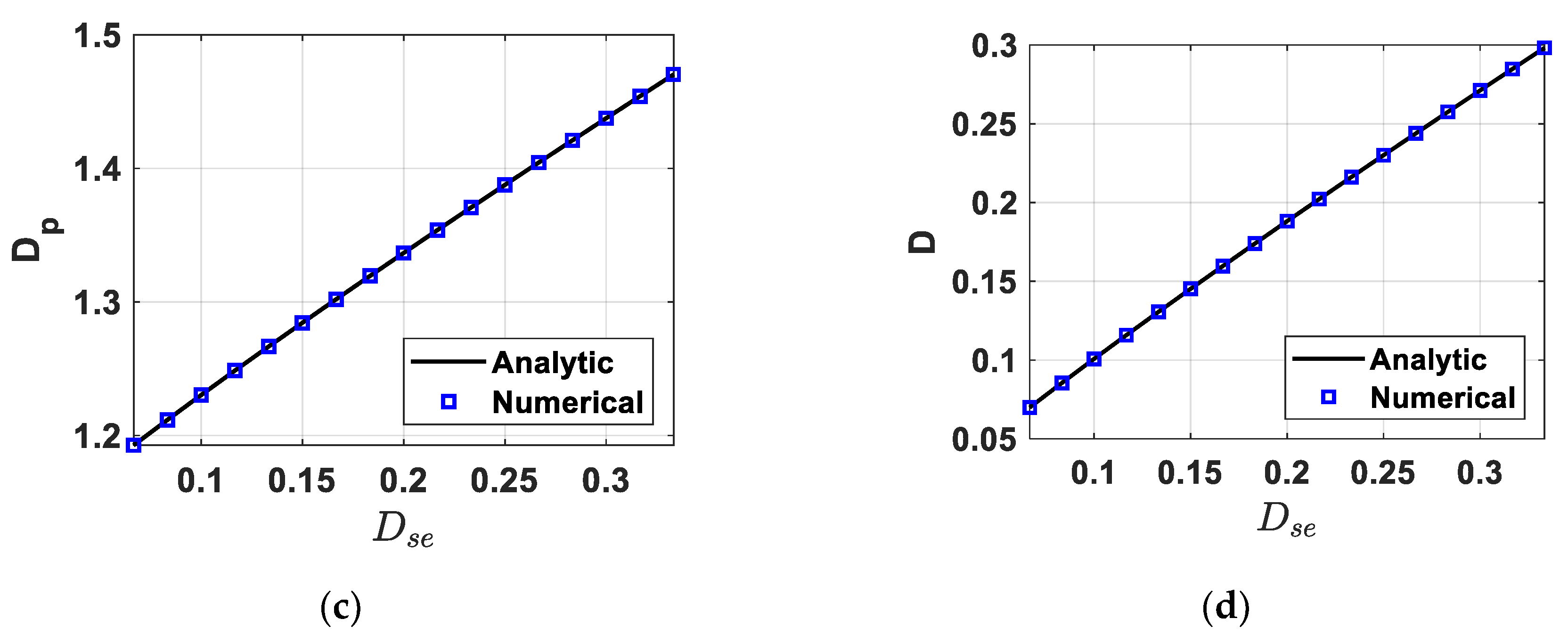
4.2. Over-Determined Case

Numerical simulations provide a means of comparing the two models under experimentally relevant b-value sampling schemes. Figure 5 shows the biexponential parameters estimated from simulated stretched exponential decays using Prony’s method (described in Section 3.2). These results are obtained using more than four samples from the uniformly spaced DW-MRI signal (including y 0 acquired at b = 0 ). In Figure 5a,b, numerical solutions progressively deviate from the analytical solutions derived for the fully determined case (Equation (22)) as the spacing of uniformly distributed samples of b values, τ , increases. Interestingly, with the decimation of the b-value sampling, all parameters { f p ,   f , D , D p } assume a near-linear relationship with respect to α ^ , particularly at larger values of α ^ . The influence of sampling on D p and D exhibits more complicated relationships with b value decimation. For example, numerical estimates of D p deviate more with the increased sampling of the b value and approach the analytical result with decimation. Numerical estimates of D show the largest deviations from the analytical expressions taking a different nonlinear shape with large overestimations at larger values of α ^ .

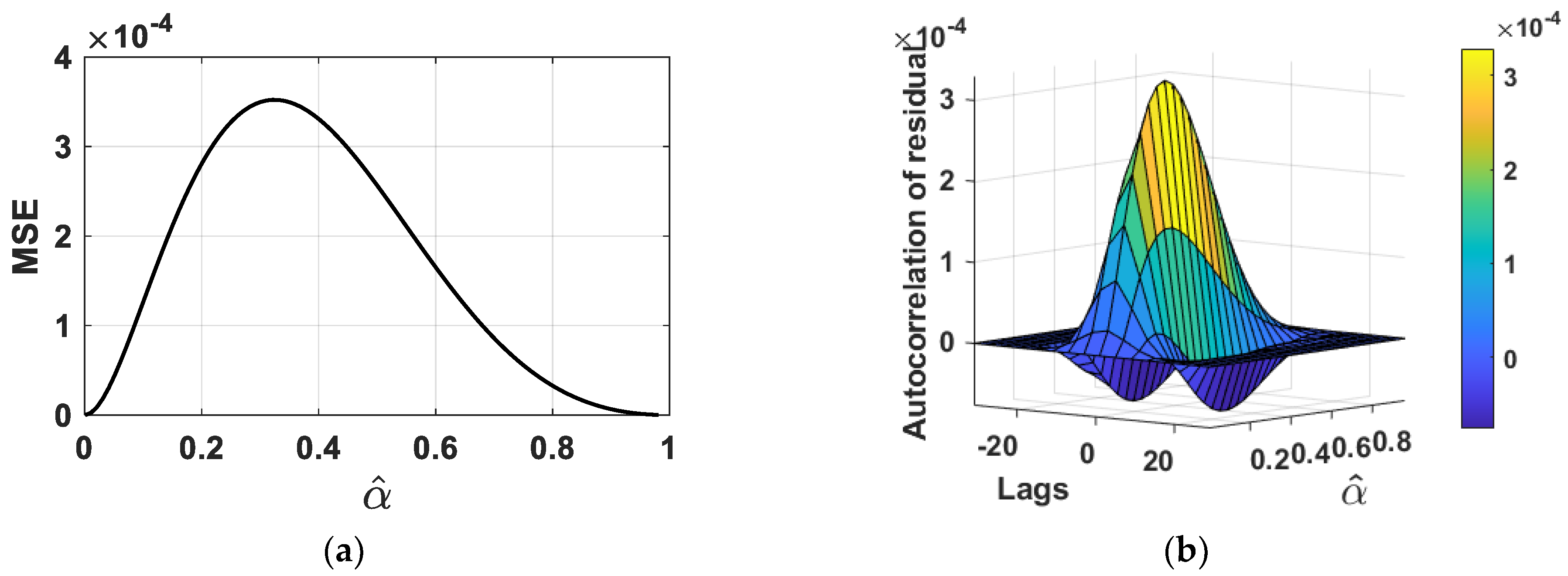
4.3. Analysis of Fit Error

For the fully determined case that uses four uniformly spaced b values (including b = 0 ) to obtain analytical solutions, zero residual is observed between decay signals from these two models. This result does not indicate that the biexponential model can perfectly represent the stretched exponential, but rather that there is an insufficient number of samples to observe deviations between the stretched exponential decay and the biexponential model.
In the overdetermined case, when more than four uniformly spaced b values (including b = 0 ) are used for the simulation, the MSE becomes nonzero, and its value varies with α ^ . Figure 6 shows an example of the MSE (panel (a) and the autocorrelation of fit error (panel (b)) over the range of α ^ using the noiseless and overdetermined b-value sampling that satisfies D s e · b m a x = 1 . The MSE (Figure 6a) remains relatively low for larger values of α ^ , suggesting difficulty in discriminating between biexponential and stretched exponential models based on goodness of fit. As values of α ^ decrease, the autocorrelation function of error (Figure 6b) shows oscillations with increasing lags, reflecting an increase in the fit error of the biexponential approximation of the stretched exponential function. The cross-section of Figure 6b at lags = 0 corresponds to the all-positive profile of MSE in Figure 6a.
The stretched exponential model, as shown by others, can be represented as a sum of multiple exponentials. Therefore, the biexponential model contains fewer exponentials than the stretched exponential model and for α ^ < 1 tends to underfit. This can be observed in Figure 6 based on the shape of the MSE as a function of α ^ .

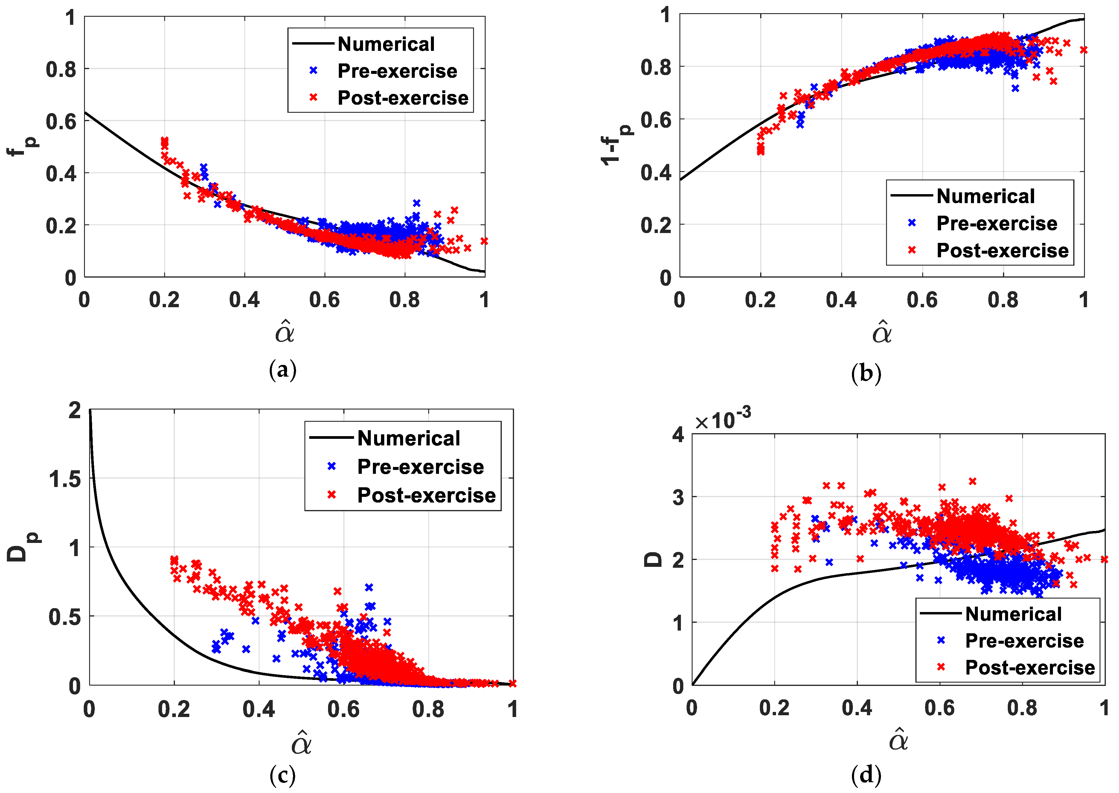
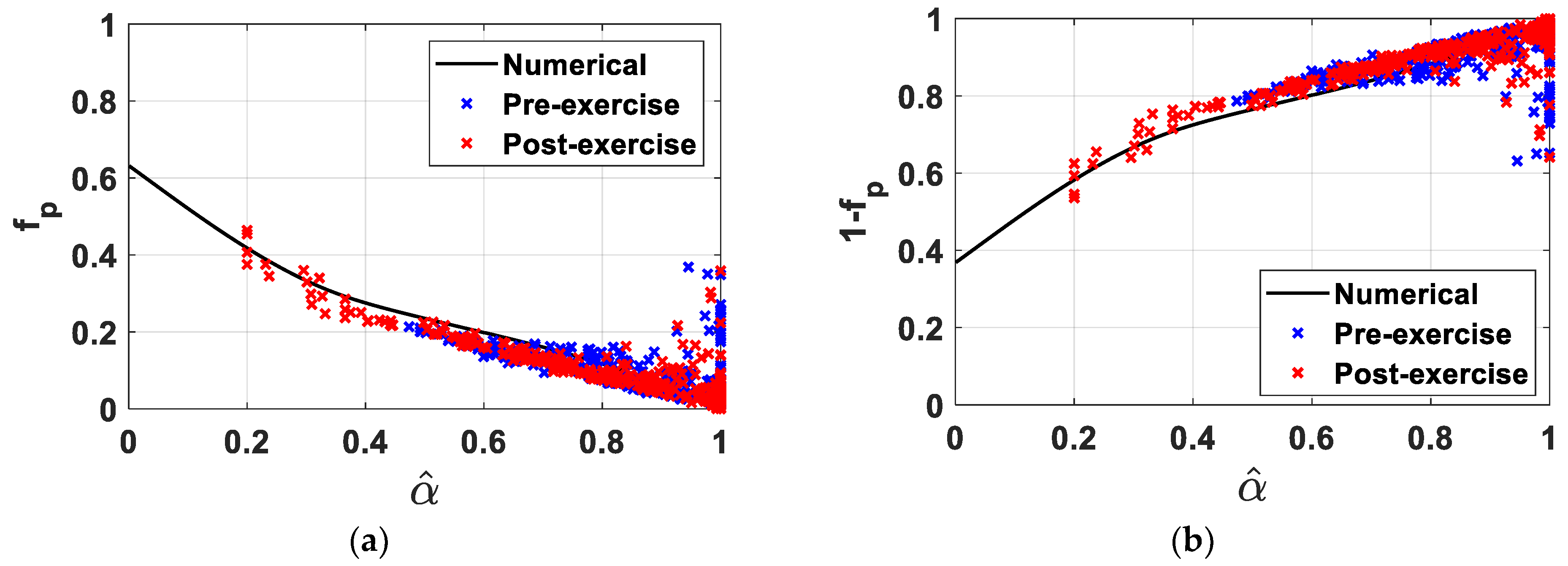
4.4. In Vivo Results

Comparisons of model fit parameters derived from experimental data from skeletal muscle demonstrated a strong resemblance to theoretical curves. Specifically, comparisons of biexponential parameters with respect to the stretched exponential parameter α ^ are shown from selected ROI’s in the rectus femoris (Figure 7) and vastus lateralis (Figure 8). The numerical estimates were obtained using the same b values for collecting experiment data and using the mean of D s e estimates derived from the stretched exponential fit for the experimental data.
For the perfusion fraction ( f p ), the experimental data shows a strong correspondence between experimental and theoretical predictions over all α ^ values, which range from 0.2 to 1. Similarly, 1 − fp shows a strong correspondence between experimental and theoretical values. The pseudo-diffusion coefficient ( D p ) and diffusion coefficient ( D ) show more scatter around the theoretical curve but largely follow the theoretical prediction. In both muscle groups displayed, these relationships were consistent under physiological conditions at rest and post-exercise hyperemia. Larger deviations of D p and D in experimental data appear to occur at lower values of α ^ . The greater variance in of D p and D can also be explained by Crammer Rao bound analysis of the biexponential model, which shows that the variance of the diffusion rate constant estimates is directly proportional to their cubed value and the quartic of the sum of D and D p , and inversely related to the quartic of their difference. Thus, the variance in D p estimates is expected to be large for large rates ( D p ) and for small separations between D and D p [25].

5. Discussion and Conclusions

The exact solutions of biexponential parameters in Equation (22) exhibit complicated nonlinear forms in terms of stretched exponential model parameters that are not easily interpreted. However, graphical comparisons provide some key insights that are useful in examining model comparisons, particularly when considering the multi-exponential nature of the stretched exponential function [19]. For example, when assessing only 4 b values spanning the full range of 1 / D s e (Figure 1), the bicomponent estimates appear almost linear with α ^ . Under these conditions, both models are indistinguishable based on the assessment of MSE (data not shown), which is not surprising since four data points are insufficient to represent more than two exponentials. Numerical simulations using the increased sampling of b values over the range of 1 / D s e (Figure 5) show how these curves approach more nonlinear relationships between biexponential parameters and α ^ . With decreased sample spacing, f p , 1 f p and D p approach curves are generated by analytical expressions using only the first four b values. In contrast, D still shows a deviation from the analytical expression, which results from the lack of sampling of larger b values in analytical expressions, which limits the amount of information used to approximate slow diffusion rate information. Thus, the analytical expression for the relationship between D and α ^ overfits rapid decay rates (e.g., perfusion information) and poorly represents slow diffusion (e.g., tissue diffusion) information.
Experimental data closely resembles the theoretical curves connecting the biexponential parameters to the stretched exponent. Perfusion ( f p ) and diffusion ( 1 f p ) fractions from the rectus femoris muscle (Figure 7) fell almost identically on the numerically generated curve. The values D p and D in the rectus femoris exhibited more noticeable deviations from the numerically generated curve, particularly during hyperemia, where the shape of the curves shows a slightly different slope. This deviation is not as apparent in the vastus lateralis muscle (Figure 8). One possible explanation for this deviation in rectus femoris results is the influence of unsuppressed and chemically shifted fat signal [23]. The single-shot echo-planar MRI readout from this sequence shifts a small amount of unsuppressed fat signal into the rectus femoris muscle creating a bias effect on biexponential fitting [24]. The vastus lateralis muscle, given the orientation of the image field of view and the geometry of the thigh, is not susceptible to this effect. Both D p and D in the vastus lateralis muscle show more dispersion around the numerical curve over the range of α ^ , which is consistent with Crammer Rao lower bound predictions of decay rate estimates in the biexponential model [25,26]. Differences in perfusion profiles between muscle groups both before and after exercise (Figure 7 and Figure 8) are attributed to differences in the demand for oxygenated blood and muscle involvement in knee extension exercise.
Although the focus of this work compares the FFD (i.e., stretched exponential) model with the ubiquitous biexponential form of the IVIM model, it should be noted that an alternative IVIM model was proposed in Le Bihan and colleagues’ original work [6], in which the perfusion term is modeled as an isotopically oriented plug flow. This condition would apply to capillary segments that are longer than the fluid particle step length within the diffusion period. Although outside of the scope of the current work, this assumption could lead to an alternative set of expressions relating the FFD model to the IVIM model. We note that in skeletal muscle, based on the average reported capillary segment length and flow velocity, the estimated time to traverse a capillary segment is ~180–525 ms, suggesting that plasma flow through the capillaries at rest might be better represented using this plug flow assumption [27]. With arteriole flow velocity being greater and segments being longer, it is likely that this kind of model is applicable to microvessels in skeletal muscle and perhaps should be considered in future work.
The problem of model selection is challenging in the space of human DW MRI-derived perfusion and diffusion applications. Models that are physically motivated by underlying physiologic properties (e.g., microvascular blood volume, microvascular blood flow rate, tissue microarchitecture, etc.) are important for leveraging these imaging tools and applying them to important research questions. However, there is a tension between the use of models that precisely represent the physical picture and those that are practical to apply to in vivo data which is inherently limited in, e.g., the sampling of b values and the signal-to-noise ratio. The stretched exponential model has demonstrated much better stability in parameter estimates than the biexponential model [28]. However, its interpretation in the context of physical properties, such as blood pool size, is much less concrete [16]. Thus, quantitative insights about the relationships between parameters from these two models and how these relationships are influenced by the sampling of the diffusion-weighted signal are useful for interpreting these models as applied to experimental data.

Author Contributions

This work involved all coauthors. J.Y. wrote the original draft, contributed to simulations, experimental analysis, the investigation, and editing; M.A.R.A. developed the analytical methodology, contributed to the investigation, and edited the manuscript; A.S. analyzed the experimental data and interpreted the results, and contributed to the discussion; D.A.R. conceived the idea, supervised the data analysis, and edited the manuscript. All authors have read and agreed to the published version of the manuscript.

Funding

This research received no external funding.

Institutional Review Board Statement

This study was carried out in accordance with the guidelines of the Declaration of Helsinki, and approved by the IRB of the National Institute of Environmental Health Science (Research Triangle Park, North Carolina).

Informed Consent Statement

All subjects gave written informed consent in accordance with the Declaration of Helsinki.

Data Availability Statement

Restrictions apply to the availability of these data. Experimental data was obtained from Intramural Research Program of the National Institute on Aging (IRP NIA) and are available with the permission from IRP NIA.

Acknowledgments

The authors thank the National Institute on Aging Intramural Research Program for permission to use data obtained from the Genetic and Epigenetic Signatures of Translational Aging Laboratory Testing (GESTALT) study for this analysis.

Conflicts of Interest

The authors declare no conflict of interest.

References

  1. Hendrickse, P.; Degens, H. The role of the microcirculation in muscle function and plasticity. J. Muscle Res. Cell Motil. 2019, 40, 127–140. [Google Scholar] [CrossRef] [PubMed] [Green Version]
  2. Neviere, R.; Mathieu, D.; Chagnon, J.L.; Lebleu, N.; Millien, J.P.; Wattel, F. Skeletal muscle microvascular blood flow and oxygen transport in patients with severe sepsis. Am. J. Respir. Crit. Care Med. 1996, 153, 191–195. [Google Scholar] [CrossRef]
  3. Lindner, J.R. Cause or Effect? Microvascular Dysfunction in Insulin-Resistant States. Circ. Cardiovasc. Imaging 2018, 11, e007725. [Google Scholar] [CrossRef] [Green Version]
  4. Toth, P.; Tarantini, S.; Csiszar, A.; Ungvari, Z. Functional vascular contributions to cognitive impairment and dementia: Mechanisms and consequences of cerebral autoregulatory dysfunction, endothelial impairment, and neurovascular uncoupling in aging. Am. J. Physiol. Heart Circ. Physiol. 2017, 312, H1–H20. [Google Scholar] [CrossRef] [PubMed] [Green Version]
  5. Bammer, R. Basic principles of diffusion-weighted imaging. Eur. J. Radiol. 2003, 45, 169–184. [Google Scholar] [CrossRef]
  6. Le Bihan, D.; Breton, E.; Lallemand, D.; Aubin, M.L.; Vignaud, J.; Laval-Jeantet, M. Separation of diffusion and perfusion in intravoxel incoherent motion MR imaging. Radiology 1988, 168, 497–505. [Google Scholar] [CrossRef] [PubMed]
  7. Hall, M. Continuity, the Bloch-Torrey equation, and Diffusion MRI. arXiv 2016, arXiv:1608.02859. [Google Scholar]
  8. Mazaheri, Y.; Afaq, A.; Rowe, D.B.; Lu, Y.; Shukla-Dave, A.; Grover, J. Diffusion-weighted magnetic resonance imaging of the prostate: Improved robustness with stretched exponential modeling. J. Comput. Assist. Tomogr. 2012, 36, 695–703. [Google Scholar] [CrossRef] [PubMed] [Green Version]
  9. Zhang, J.; Suo, S.; Liu, G.; Zhang, S.; Zhao, Z.; Xu, J.; Wu, G. Comparison of Monoexponential, Biexponential, Stretched-Exponential, and Kurtosis Models of Diffusion-Weighted Imaging in Differentiation of Renal Solid Masses. Korean J. Radiol. 2019, 20, 791–800. [Google Scholar] [CrossRef]
  10. Seo, N.; Chung, Y.; Park, Y.; Kim, E.; Hwang, J.; Kim, M.-J. Liver fibrosis: Stretched exponential model outperforms mono-exponential and bi-exponential models of diffusion-weighted MRI. Eur. Radiol. 2018, 28, 1–11. [Google Scholar] [CrossRef]
  11. Bai, Y.; Lin, Y.; Tian, J.; Shi, D.; Cheng, J.; Haacke, E.M.; Hong, X.; Ma, B.; Zhou, J.; Wang, M. Grading of Gliomas by Using Monoexponential, Biexponential, and Stretched Exponential Diffusion-weighted MR Imaging and Diffusion Kurtosis MR Imaging. Radiology 2015, 278, 496–504. [Google Scholar] [CrossRef]
  12. Li, C.; Ye, J.; Prince, M.; Peng, Y.; Dou, W.; Shang, S.; Wu, J.; Luo, X. Comparing mono-exponential, bi-exponential, and stretched-exponential diffusion-weighted MR imaging for stratifying non-alcoholic fatty liver disease in a rabbit model. Eur. Radiol. 2020, 30, 6022–6032. [Google Scholar] [CrossRef]
  13. Dietrich, O.; Biffar, A.; Baur-Melnyk, A.; Reiser, M.F. Technical aspects of MR diffusion imaging of the body. Eur. J. Radiol. 2010, 76, 314–322. [Google Scholar] [CrossRef]
  14. Stejskal, E.O.; Tanner, J.E. Spin Diffusion Measurements: Spin Echoes in the Presence of a Time—Dependent Field Gradient. J. Chem. Phys. 1965, 42, 288–292. [Google Scholar] [CrossRef] [Green Version]
  15. Jensen, J.H.; Helpern, J.A. Effect of gradient pulse duration on MRI estimation of the diffusional kurtosis for a two-compartment exchange model. J. Magn. Reson. 2011, 210, 233–237. [Google Scholar] [CrossRef] [Green Version]
  16. Reiter, D.A.; Adelnia, F.; Cameron, D.; Spencer, R.G.; Ferrucci, L. Parsimonious modeling of skeletal muscle perfusion: Connecting the stretched exponential and fractional Fickian diffusion. Magn. Reson. Med. 2021, 86, 1045–1057. [Google Scholar] [CrossRef] [PubMed]
  17. Ingo, C.; Sui, Y.; Chen, Y.; Parrish, T.B.; Webb, A.G.; Ronen, I. Parsimonious continuous time random walk models and kurtosis for diffusion in magnetic resonance of biological tissue. Front. Phys. 2015, 3. [Google Scholar] [CrossRef] [PubMed] [Green Version]
  18. Bennett, K.M.; Schmainda, K.M.; Bennett, R.T.; Rowe, D.B.; Lu, H.; Hyde, J.S. Characterization of continuously distributed cortical water diffusion rates with a stretched-exponential model. Magn. Reson. Med. 2003, 50, 727–734. [Google Scholar] [CrossRef] [PubMed]
  19. Berberan-Santos, M.N.; Valeur, B. Luminescence decays with underlying distributions: General properties and analysis with mathematical functions. J. Lumin. 2007, 126, 263–272. [Google Scholar] [CrossRef]
  20. Johnston, D.C. Stretched exponential relaxation arising from a continuous sum of exponential decays. Phys. Rev. B 2006, 74, 184430. [Google Scholar] [CrossRef] [Green Version]
  21. Kay, S.M. Fundamentals of Statistical Signal Processing: Estimation Theory; Prentice-Hall, Inc.: Upper Saddle River, NJ, USA, 1993. [Google Scholar]
  22. Fernández Rodríguez, A.; de Santiago Rodrigo, L.; López Guillén, E.; Rodríguez Ascariz, J.M.; Miguel Jiménez, J.M.; Boquete, L. Coding Prony’s method in MATLAB and applying it to biomedical signal filtering. BMC Bioinf. 2018, 19, 451. [Google Scholar] [CrossRef] [PubMed] [Green Version]
  23. Adelnia, F.; Shardell, M.; Bergeron, C.M.; Fishbein, K.W.; Spencer, R.G.; Ferrucci, L.; Reiter, D.A. Diffusion-weighted MRI with intravoxel incoherent motion modeling for assessment of muscle perfusion in the thigh during post-exercise hyperemia in younger and older adults. NMR Biomed. 2019, 32, e4072. [Google Scholar] [CrossRef]
  24. Cameron, D.; Bouhrara, M.; Reiter, D.A.; Fishbein, K.W.; Choi, S.; Bergeron, C.M.; Ferrucci, L.; Spencer, R.G. The effect of noise and lipid signals on determination of Gaussian and non-Gaussian diffusion parameters in skeletal muscle. NMR Biomed. 2017, 30, 3718. [Google Scholar] [CrossRef] [Green Version]
  25. Anjum, M.A.R.; Gonzalez, F.M.; Swain, A.; Leisen, J.; Hosseini, Z.; Singer, A.; Umpierrez, M.; Reiter, D.A. Multi-component T2∗ relaxation modelling in human Achilles tendon: Quantifying chemical shift information in ultra-short echo time imaging. Magn. Reson. Med. 2021, 86, 415–428. [Google Scholar] [CrossRef] [PubMed]
  26. Anjum, M.A.R. High-Resolution Multidimensional Parametric Estimation for Nuclear Magnetic Resonance Spectroscopy; Victoria University of Wellington: Wellington, New Zealand, 2019. [Google Scholar]
  27. Ivanov, K.P.; Kalinina, M.K.; Levkovich Yu, I. Blood flow velocity in capillaries of brain and muscles and its physiological significance. Microvasc. Res. 1981, 22, 143–155. [Google Scholar] [CrossRef]
  28. Reiter, D.A.; Magin, R.L.; Li, W.; Trujillo, J.J.; Pilar Velasco, M.; Spencer, R.G. Anomalous T2 relaxation in normal and degraded cartilage. Magn. Reson. Med. 2016, 76, 953–962. [Google Scholar] [CrossRef] [PubMed] [Green Version]
Figure 1. Analytical solutions from Equation (22) (Section 3.1) and numerical solutions from Equation (23) are shown for biexponential model parameters (a) fp, (b) 1 − fp, (c) D0, and (d) D, as functions of the stretched exponent α ^ , both for b   = 0, 1, 2, 3 and D s e = 1 / 3 .
Mathematics 09 01963 g001
Figure 2. Analytical solutions from Equation (22) (Section 3.1) and numerical solutions from Equation (23) are shown for biexponential model parameters (a) fp, (b) 1 − fp, (c) D0, and (d) D, as functions of the stretched exponent D s e , both for b   = 0, 1, 2, 3 and α ^ = 0.9 .
Mathematics 09 01963 g002aMathematics 09 01963 g002b
Figure 3. Analytical results from Equation (22) are shown for biexponential model parameters (a) fp, (b) 1 − fp, (c) D0, and (d) D, as functions of stretched exponential parameters D s e and α ^ , when b = 0, 1, 2, 3 and D s e · b m a x 1 .
Mathematics 09 01963 g003
Figure 4. Pole behavior of the biexponential model for uniformly spaced b values of b = 0, 1, 2, 3 and D s e = 1 / b m a x ; (b) is the top view of (a). The red trajectory is associated with the pole ( ρ 1 = e D p ) that corresponds to the pseudo-diffusion with amplitude f p and the blue trajectory is associated with the pole ( ρ 2 = e D ) that corresponds to the true diffusion with amplitude f . The arrows indicate the direction of the pole trajectory as α ^ increases from 0+ to 1.
Mathematics 09 01963 g004
Figure 5. Biexponential parameter estimates as a function of the stretched exponent α ^ . Simulations were implemented by taking uniformly spaced b values with b m a x = 400 and D s e = 1 / b m a x . Lines encoded with different colors correspond to the sampling interval of b values, τ , which took discrete values of 1, 5, 10, 20, 30, and 50. The analytical solutions (in black lines) were implemented with b = 0 , 1 , 2 , 3 and D s e = 1 / 400 .
Mathematics 09 01963 g005
Figure 6. Mean squared error calculated from simulations using a b values span between 1 and 20 and uniformly spaced by 1, and D s e = 1 / b m a x . (a) MSE as a function of α ^ ; (b) Autocorrelation of fit error at various lags and α ^ .
Mathematics 09 01963 g006
Figure 7. Experimental traces of biexponential model parameters obtained from ROI in the rectus femoris at baseline and post-exercise, superimposed by numerical traces. Both numerical and experimental analysis used: b = 0, 3, 7, 10, 15, 20, 25, 30, 40, 50, 70, 100, 200, and 400 s / mm 2 .
Mathematics 09 01963 g007
Figure 8. Experimental traces of biexponential model parameters obtained from ROI in the vastus lateralis at baseline and post-exercise, superimposed by numerical traces. Both numerical and experimental analysis used: b = 0, 3, 7, 10, 15, 20, 25, 30, 40, 50, 70, 100, 200, and 400 s / mm 2 .
Mathematics 09 01963 g008aMathematics 09 01963 g008b
Publisher’s Note: MDPI stays neutral with regard to jurisdictional claims in published maps and institutional affiliations.

