Discrete Time Hybrid Semi-Markov Models in Manpower Planning

Abstract

Discrete time Markov models are used in a wide variety of social sciences. However, these models possess the memoryless property, which makes them less suitable for certain applications. Semi-Markov models allow for more flexible sojourn time distributions, which can accommodate for duration of stay effects. An overview of differences and possible obstacles regarding the use of Markov and semi-Markov models in manpower planning was first given by Valliant and Milkovich (1977). We further elaborate on their insights and introduce hybrid semi-Markov models for open systems with transition-dependent sojourn time distributions. Hybrid semi-Markov models aim to reduce model complexity in terms of the number of parameters to be estimated by only taking into account duration of stay effects for those transitions for which it is useful. Prediction equations for the stock vector are derived and discussed. Furthermore, the insights are illustrated and discussed based on a real world personnel dataset. The hybrid semi-Markov model is compared with the Markov and the semi-Markov models by diverse model selection criteria.

1. Introduction

Manpower planning is a key aspect of modern human resources management. The principal aim of manpower planning is the development of plans dealing with future human resource requirements. In this way, an effective manpower planning policy can avoid future shortages and excesses of staff members. Such an imbalance between the actual and the required staff is highly undesirable because it would lead to higher costs and/or less profits. Since manpower planning itself is concerned with the description and prediction of large groups of employees, whose behaviour can be unpredictable at the individual level, it is only natural to study aggregated data, where statistical patterns may appear. So, it is no surprise that the use of mathematical models for manpower planning can be traced back to at least 1779 when Rowe used a career-modeling plan in the Royal Marines [1].

Since the 1960s and the dawn of the computer age, such models have become an essential tool for the modern manager. Pioneering work concerning mathematical approaches for manpower planning was carried out by Vajda [2,3] and Bartholomew [4,5], whereas Almond and Young [6] were the first to study a real world application of an open homogeneous Markov chain model. Since then, various other manpower planning model approaches have been considered. In the work of Vassiliou [7], the non-homogeneous Markov system was introduced. This idea was expanded upon by Vasilliou et al. [8]. Other work regarding non-homogeneous discrete time (semi-)Markov models includes the works of Papadopoulou [9] and Dimitriou et al. [10] as well as continuous time (semi-)Markov models by McClean et al. [11,12], Papadopoulou et al. [13] and Mehlmann [14]. It is important to remark that the scope of those models is not limited to humans [7], as is the case in manpower planning, but that it can be any biological being or object. Some examples of other populations modeled by this class of stochastic processes [15] include ecological modeling [16] and biological Markov population models [17] and financial applications [18]. It is remarkable that, until recently, discrete time homogeneous semi-Markov models were somewhat neglected in manpower planning.

One of the assumptions of a Markov model is that the length of time a person stays in a state $S_i$ before going to another state $S_j$ only depends on the state $S_i$ itself. Moreover, the waiting time distribution, often called the sojourn time distribution, exhibits the memoryless property. Which means that it does not account for possible duration of stay effects. In this case, the sojourn time distribution is in fact a geometric distribution. However, in practice those assumptions may pose an unrealistic limitation. An alternative model that may solve those problems is a semi-Markov model, which can be viewed as a natural extension of a Markov model. In recent years, the use of discrete time semi-Markov models became more and more popular in various fields such as reliability and survival analysis [19], DNA analysis [20,21], disability insurance [22], credit risk [23,24,25,26], and wind speed and tornado modeling [27,28]. Moreover, insights regarding discrete time semi-Markov models contribute to the use of continuous time semi-Markov models [29].

Markov models and semi-Markov models both have advantages: Markov models are less complex and more transparent. In the manpower planning context, for example, this makes a classical Markov model easier to interpret and understand for a manager. Semi-Markov models, on the other hand, allow capturing duration of stay effects due to their more general sojourn distributions. This provides motivation to build hybrid models that incorporate the best of both approaches. In the previous work of Guédon, so-called hidden hybrid semi-Markov chains are presented that combine Markovian states with semi-Markovian states [30]. Since it is possible that, for a particular state, some of the transitions are Markovian while other transitions are semi-Markovian [22], the present paper introduces the concepts of Markovian transitions and semi-Markovian transitions. In this way, Markovian and semi-Markovian transitions are a further refinement of Markovian and semi-Markovian states.

Furthermore, both Markov and semi-Markov models require longitudinal data for their parameter estimation. In practice, however, longitudinal data are often left truncated or right censored, which may lead to estimation problems [31], especially in a semi-Markovian context, where more general sojourn time distributions are allowed. Previous works [11,32] suggest alternative approaches [23,33] to deal with this drawback, such as restricting the analyses to the items for which there is complete information, artificially truncating the data or using adapted formulas for the estimation of the parameters.

In this paper, we discuss the advantages and disadvantages of Markov and semi-Markov manpower planning models in Section 2. In Section 3, we present the so-called hybrid semi-Markov model, which uses a mix of Markov (geometric) and more general (Weibull) sojourn time distributions, offering some advantages: the hybrid semi-Markov model allows for capturing duration of stay effects where useful and reduces the number of parameters to estimate, where possible. In this way, the hybrid semi-Markov model enables one to improve on the semi-Markov model in case the amount of available data is limited. Finally, in Section 4, we use a real world personnel dataset to illustrate our insights. The hybrid semi-Markov model is compared with the Markov model as well as with the semi-Markov model based on several criteria.

2. Markov and Semi-Markov Manpower Planning Models

To model a manpower system, one has to account for three different types of flows: the incoming flows (recruitments), the internal flows between the different personnel categories and the outgoing flows (wastage). We consider $G+1$ states, given by G personnel categories and one absorbing state W, corresponding to the wastage. First of all, the classical Markov model [4] will be discussed; afterwards, a semi-Markov model for manpower planning based on [19] will be proposed. An interesting reference regarding (semi-)Markov processes is [34]. The discussion on the classical Markov model (in Section 2.1) and the semi-Markov model (in Section 2.2) contributes in defining the new hybrid semi-Markov model in Section 3.

2.1. Markov Model

All models in this section are Markov processes and generalizations thereof, such as semi-Markov processes. However, all models have their limitations and are subjected to restrictions. In this setting, one of the assumptions we make is the so-called Markov property, which states that the probability of reaching a future state is independent of the past states and only depends on the present state. For a second-order Markov chain, this probability of entering a state at time $t+1$ also depends on the state at time $t-1$. To assess the Markov property, we will use Equation (1) below, which tests a first-order against a second-order Markov chain. The use of a classical Markov model without meeting the first-order assumption may lead to false conclusions and incorrect analysis results. An extensive discussion about the often overlooked need to check for the Markov property can be found in [35]. For a given stochastic process ${\left\{X_t\right\}}_t$ with $G+1$ states $\{S_1,\cdots ,S_{G+1}\}$ and data over a time horizon $[0,T]$, we will use the following ${\chi }^2$ goodness of fit test to verify the first-order assumption, as described in [35,36],

$${\chi }_e^2=\sum _{i\in \mathcal{G}}\sum _{j\in \mathcal{G}}\sum _{l\in \mathcal{G}}{n}_{ij}\frac{{(\widehat{p_{ijl}}-\widehat{p_{jl}})}^2}{\widehat{p_{jl}}}$$

(1)

with index set $\mathcal{G}=\{1,2,\cdots ,G,G+1\}$ and $n_{ij}={\sum }_{t=0}^{T-1}{\sum }_{k=0}^m{n}_{ij}(t,k)$ , where $n_{ij}(t,k)$ is the number of persons that are at time t in the state $S_i$ with grade seniority k and at time $t+1$ in state $S_j$ and m is the maximal grade seniority observed in the database. $\widehat{p_{jl}}$ is the maximum likelihood estimator of the transition probability $p_{jl}$ with $N_j\left(t\right)={\sum }_{i\in \mathcal{G}}{\sum }_{k=0}^m{n}_{ij}(t-1,k)$ being the number of persons in state $S_j$ at time t , where $\widehat{p_{ijl}}$ is the maximum likelihood estimator of the transition probability $p_{ijl}$ and where $n_{ijl}(t,k)$ is the number of persons that are at time t in the state $S_i$ with grade seniority k at time $t+1$ in the state $S_j$ and at time $t+2$ in the state $S_l$:

$$\widehat{p_{jl}}=\frac{{\sum }_{t=0}^{T-1}{\sum }_{k=0}^m{n}_{jl}(t,k)}{{\sum }_{t=0}^{T-1}{N}_j\left(t\right)}.$$

(2)

$$p_{jl}=Pr(X_t=S_l|X_{t-1}=S_j)$$

(3)

$$\widehat{p_{ijl}}=\frac{{\sum }_{t=0}^{T-2}{\sum }_{k=0}^m{n}_{ijl}(t,k)}{{\sum }_{t=0}^{T-2}{\sum }_{k=0}^m{n}_{ij}(t,k)}.$$

(4)

$$p_{ijl}=Pr(X_{t+2}=S_l|X_{t+1}=S_j,X_t=S_i)$$

(5)

Only non-zero $\widehat{p_{jl}}$ are taken into account for computing ${\chi }_e^2$. Under the assumption that the Markov property is satisfied, i.e., that we are looking for a Markov chain of order 1, the test statistic ${\chi }_e^2$ has a ${\chi }^2$-distribution with ${(G+1)}^3$ degrees of freedom. If this assumption holds, we can proceed with the classical Markov approach, in which transition probabilities are assumed to be equal for individuals within a category.

The use of time homogeneous Markov chains in manpower planning is well-known (see, for example, [4]) . Given the G states corresponding to different personnel categories $S_1,\cdots ,S_G$ and a wastage state $W=S_{G+1}$, one can define a Markov process ${\left\{X_t\right\}}_t$ on those states with transition probabilities $p_{jl}$ that can be estimated by Equation (2). If we denote the stock vector at time t by $\mathbf{N}\left(t\right)=(N_1\left(t\right),N_2\left(t\right),\cdots ,N_G\left(t\right),W\left(t\right))$, and write $\mathbf{R}\left(t\right)=(R_1\left(t\right),R_2\left(t\right),\cdots ,R_G\left(t\right),0)$ for the recruitment vector at time t, then we obtain the prediction equation [4] for the stocks at time $t+1$ :

$$\mathbf{N}(t+1)=\mathbf{N}\left(t\right)·\mathbf{P}+\mathbf{R}(t+1),$$

(6)

where $\mathbf{P}$ is the matrix with elements $\widehat{p_{jl}}$.

Due to their simplicity, time homogeneous Markov chain models are used in a wide variety of domains and applications. As there are relatively few parameters to estimate in a time homogeneous Markov chain model, they are not too data demanding. However, on the other hand, they cannot be used to account for duration of stay effects and they are less flexible due to the so-called memoryless property, which implies that their sojourn time distributions are geometrical distributed by construction. This shortcoming is accounted for in semi-Markov models.

2.2. Semi-Markov Model

Again, consider a system with a finite number of states $\{S_1,\cdots ,S_G,S_{G+1}\}$ and let us denote the set of indices by $\mathcal{G}=\{1,2,\cdots ,G,G+1\}$. Furthermore, let $T_n$ and $J_n$ denote, respectively, the time of the n-th transition and the state occupied after the n-th transition.

A semi-Markov process is equivalent to a Markov renewal process [37] and is completely determined by an initial distribution $\mathbf{\delta }=({\delta }_1,\cdots {\delta }_G,{\delta }_{G+1})$ and a discrete semi-Markov kernel $\mathbf{q}=(q_{ij}\left(k\right):i,j\in \mathcal{G},k\in \mathbb{N})$ where

$$q_{ij}\left(k\right)=Pr(J_{n+1}=S_j,T_{n+1}-T_n=k\mid J_n=S_i).$$

(7)

It can be shown that ${\left\{J_n\right\}}_n$ itself is a Markov chain via

$$p_{ij}^{\infty }=Pr(J_{n+1}=S_j\mid J_n=S_i),$$

(8)

i.e., $p_{ij}^{\infty }$ is the probability, starting from $S_i$, that the next state will eventually be $S_j$, regardless of the duration time. We write ${\mathbf{P}}^{\infty }=(p_{ij}^{\infty }:i,j\in \mathcal{G})$ for the associated transition matrix. This allows for the following decomposition:

$$q_{ij}\left(k\right)=p_{ij}^{\infty }{f}_{ij}\left(k\right)$$

(9)

where $\mathbf{f}=(f_{ij}\left(k\right):i,j\in \mathcal{G},k\in \mathbb{N})$ consists of the sojourn time distributions, conditioned by the next state to be visited:

$$f_{ij}\left(k\right)=Pr(T_{n+1}-T_n=k\mid J_n=S_i,J_{n+1}=S_j)$$

(10)

A few remarks are in order at this point. First of all, only actual transitions are accounted for, in the sense that transitions to the same state are prohibited, so that $p_{ii}^{\infty }=0$ for every $i\in \mathcal{G}$. Furthermore, instantaneous transitions are not allowed either: the chain has to spend at least one unit of time in a state, which corresponds to $f_{ij}\left(0\right)=q_{ij}\left(0\right)=0$ for every $i,j\in \mathcal{G}$.

The main difference in regard to the Markov chain model is the fact that the sojourn time distributions $\mathbf{f}$ can be any discrete distribution, incorporating the possible duration of stay effects. Note that a Markov chain with transition matrix $\mathbf{P}=(p_{ij}:i,j\in \mathcal{G})$ itself can be viewed as a semi-Markov chain with geometrically distributed sojourn times for which

$$q_{ij}\left(k\right)=\left\{\begin{array}{cc}{p}_{ij}{p}_{ii}^{k-1}\hfill & \mathrm{if} i\ne j \mathrm{and} k\in {\mathbb{N}}_0\hfill \\ 0\hfill & \mathrm{elsewhere}.\hfill \end{array}\right.$$

(11)

In order to use this framework for a manpower planning model, one starts in the same way as in the case of a Markov chain model with dividing the population in $G+1$ states and determining the corresponding stock vector $\mathbf{N}\left(t\right)$. In contrast with the Markov chain model, we incorporate the grade seniority of the employees in our model. Instead of a vector $\mathbf{N}\left(t\right)$ consisting of the total number of people in each personnel category at time t, every entry of $\mathbf{N}\left(t\right)$ corresponds to a vector of a certain length m containing the number of employees with seniority l, with $1\le l\le m$. This disaggregation of the entries of $\mathbf{N}\left(t\right)$ results in a matrix, whose columns will be denoted by $\mathbf{N}(t,k)$ as in Figure 1. So, the first column, $\mathbf{N}(t,0)$, corresponds to the employees with grade seniority 0 at time t, the second column, $\mathbf{N}(t,1)$, corresponds to the employees with grade seniority 1 at time t, ... up to the $m+1$-th column that corresponds to the employees with grade seniority m at time t , where m is the maximal grade seniority observed in the database. We will call this matrix the seniority based stock matrix. Note that $N_i(t,k)$ corresponds to the number of employees in state $S_i$ with grade seniority k at time t and that ${\sum }_{k=0}^m{N}_i(t,k)=N_i\left(t\right)$ for each $i\in \mathcal{G}$ and every $t\in \mathbb{N}$. The vectors $\mathbf{N}(t,k)$ enable the expression of the prediction equation for the stock vector as in Theorem 2. An equivalent approach is presented in [8], where the semi-Markov system is transformed into a Markov system. While the present paper considers a separate vector $\mathbf{N}(t,k)$ for each grade seniority k, in [8], this information is gathered into one vector.

Now, we can estimate a discrete semi-Markov kernel $\mathbf{q}$ using the maximum likelihood estimator [19]:

$$\widehat{q_{ij}\left(k\right)}=\frac{{\sum }_{t=0}^{T-1}{n}_{ij}(t,k)}{n_i}$$

(12)

where $n_i={\sum }_{j\ne i}{\sum }_{t=0}^{T-1}{\sum }_{k=0}^m{n}_{ji}(t,k)$, i.e., the total number of visits to state i. Furthermore, we can use this $\mathbf{q}$ to calculate the grade seniority transition matrices $\mathbf{P}\left(k\right)=(P_{ij}\left(k\right):i,j\in \mathcal{G})$, the one-step ahead transition matrix for group members with grade seniority k, is defined by:

$$P_{ij}\left(k\right)=Pr(J_{n+1}=j,T_{n+1}-T_n=k\mid J_n=i,T_{n+1}-T_n>k-1)$$

(13)

In practice, $\mathbf{P}\left(k\right)$ can be calculated in the following way.

Theorem 1.

For all k such that ${\sum }_{h\in \mathcal{G}}{\sum }_{m=0}^{k-1}{q}_{ih}\left(m\right)\ne 1$ we have

$$P_{ij}\left(k\right)=\frac{q_{ij}\left(k\right)}{1-{\sum }_{h\in \mathcal{G}}{\sum }_{m=0}^{k-1}{q}_{ih}\left(m\right)}$$

(14)

Proof.

$$\begin{array}{cc}\hfill P_{ij}\left(k\right)& =Pr(J_{n+1}=j,T_{n+1}-T_n=k\mid J_n=i,T_{n+1}-T_n>k-1)\hfill \\ \hfill & =\frac{Pr(J_{n+1}=j,T_{n+1}-T_n=k\mid J_n=i)}{Pr(T_{n+1}-T_n>k-1\mid J_n=i)}\hfill \\ \hfill & =\frac{Pr(J_{n+1}=j,T_{n+1}-T_n=k\mid J_n=i)}{1-Pr(T_{n+1}-T_n\le k-1\mid J_n=i)}\hfill \\ \hfill & =\frac{q_{ij}\left(k\right)}{1-{\sum }_{h\in \mathcal{G}}{\sum }_{m=0}^{k-1}{q}_{ih}\left(m\right)}\hfill \end{array}$$

□

Combining all of the above, we arrive at:

Theorem 2.

For a semi-Markov system, the prediction equation for the stock vector at time $t+1$ is as follows:

$$\mathbf{N}(t+1)=\sum _{k=0}^m\left(\mathbf{N}(t,k)·\mathbf{P}\left(k\right)\right)+\mathbf{R}(t+1),$$

(15)

where $\mathbf{N}(t,k)$ is the stock vector of people with grade seniority k at time t, $\mathbf{R}(t+1)$ is the recruitment vector at time $t+1$, $\mathbf{P}\left(k\right)$ is the one-step ahead transition matrix for people with grade seniority k and m is the maximum of all grade seniorities.

At first glance, it would seem that the semi-Markov model is a preferable model due to its more flexible sojourn time distributions and its greater generality. However, to build a semi-Markov model, one has to estimate more parameters, such that a sufficiently long time series of data may be necessary to avoid problems with overfitting [38]. This may limit the utility of semi-Markov modeling in manpower planning as a data horizon of, for example, less than ten years may be insufficient for the realization of some transitions and so for the required data for estimating the semi-Markov kernel $\mathbf{q}$.

3. Hybrid Semi-Markov Model

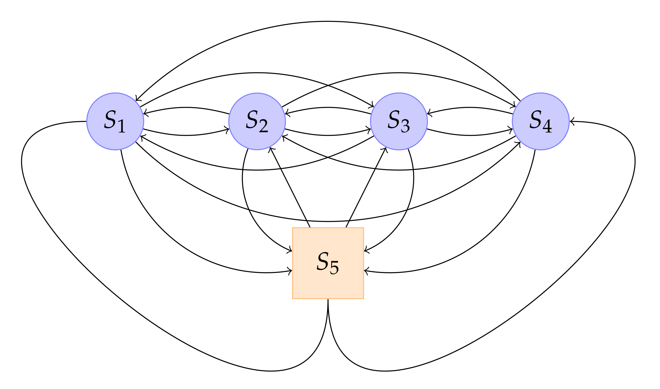
In Section 2.2, we note that a Markov chain with transition matrix $\mathbf{P}=(p_{ij}:i,j\in \mathcal{G})$ can be viewed as a semi-Markov chain, i.e., a semi-Markov chain can be considered as an extension of a Markov chain, where more general and flexible sojourn time distributions are allowed. However, in practice, it can be difficult to decide which approach is more adequate to model the manpower system in question. Due to its greater generality, the semi-Markov chain may look as the most preferable model at first sight. However, in practice, the data requirements to result in accurate parameter estimates may limit the utility of semi-Markov models in manpower planning [38]. For these reasons, the presented hybrid semi-Markov model examines, for each pair of states $(S_i,S_j)$, whether the transition from $S_i$ to $S_j$ can be considered as a Markov transition or should be modeled as a semi-Markov transition. In order to make an adequate choice for a particular transition from $S_i$ to $S_j$ between a Markov and a semi-Markov approach, one can use a technique which was introduced in [22] and which is briefly discussed below.

The semi-Markov hypothesis is tested at the level of the sojourn time distributions $f_{ij}$. A transition from $S_i$ to $S_j$ can be considered Markovian if its corresponding sojourn time $f_{ij}$ is geometrically distributed. Under the geometrical hypothesis, the equality $f_{ij}\left(2\right)=f_{ij}\left(1\right)(1-f_{ij}\left(1\right))$ holds and a significant deviation of $f_{ij}\left(1\right)(1-f_{ij}\left(1\right))-f_{ij}\left(2\right)$ from zero has to be seen as evidence to the contrary, i.e., evidence in favor of a (more general) sojourn time distribution. The test statistic, as introduced in [22], is given by:

$${\widehat{S}}_{ij}=\frac{\sqrt{n_{ij}}({\widehat{f}}_{ij}\left(1\right)\ast (1-{\widehat{f}}_{ij}\left(1\right))-{\widehat{f}}_{ij}\left(2\right))}{\sqrt{{\widehat{f}}_{ij}\left(1\right){(1-{\widehat{f}}_{ij}\left(1\right))}^2(2-{\widehat{f}}_{ij}\left(1\right))}}$$

(16)

where $n_{ij}={\sum }_{t=0}^{T-1}{\sum }_{k=0}^m{n}_{ij}(t,k)$ denotes the observed total number of transitions from $S_i$ to $S_j$ and where $\widehat{f_{ij}}\left(k\right)$ is the maximum likelihood estimator of the probability $f_{ij}\left(k\right)$ (see [19]):

$$\widehat{f_{ij}}\left(k\right)=\frac{{\sum }_{t=0}^{T-1}{n}_{ij}(t,k)}{n_{ij}}.$$

(17)

Under the geometrical hypothesis $H_0$, the test statistic ${\widehat{S}}_{ij}$ is asymptotically normally distributed.

Note that for a system with $G+1$ states, this test has to be run $(G+1)*G$ times as this test permits us to make a decision about the sojourn time distribution for each $f_{ij}$ individually, which allows for a so-called hybrid semi-Markov model—a semi-Markov model that incorporates the sojourn time distributions of the classical Markov model for those pairs $(S_i,S_j)$ where geometric sojourn time distributions may be assumed and that enables the use of more general sojourn time distributions for those pairs $(S_i,S_j)$ where necessary. This approach can be seen as a further generalization of techniques used in [22,39], where the same criterion was used to make a decision about the sojourn time distributions at the level of the states instead of the transitions. Since the sojourn time distribution is determined per pair $(S_i,S_j)$, and hence for each possible transition, the hybrid semi-Markov model is based on transition-dependent sojourn time distributions. In this way, we can construct a model that unites the best of the Markovian and (pure) semi-Markovian worlds, as we will only have to estimate extra parameters of the sojourn time distributions if those parameters might improve the goodness of fit.

Previous studies concerning semi-Markov models often used the discrete Weibull distribution [19] whenever the geometrical hypothesis is rejected. The choice for the discrete Weibull distribution is motivated by the fact that the discrete Weibull distribution can be viewed as a more flexible generalization of the geometric distribution [40]:

$$\begin{array}{cc}\hfill & \mathbf{CMF}dweibull(k,\alpha ,\beta )=1-{\alpha }^{{(k+1)}^{\beta }}\hfill \end{array}$$

(18)

$$\begin{array}{cc}\hfill & \mathbf{CMF}geometric(k,p)=1-{(1-p)}^{(k+1)}\hfill \end{array}$$

(19)

so $geometric(k,p)=dweibull(k,1-p,1)$.

Note that, in the semi-Markov setting, the prediction equation of the stock vector (Equation (15)) is nothing more than a generalization of the prediction equation of the stock vector in the Markov setting (Equation (1)), as in the latter case the $\mathbf{P}\left(k\right)$ are equal for all k. So, to arrive at the prediction equation for the stock vector of the hybrid semi-Markov model, one can recycle Equation (15), where $P_{ij}\left(k\right)$ will be dependent on k due to the sojourn time distributions associated with the $(S_i,S_j)$ for which the Markov hypothesis does not hold.

A procedure to decide on whether to use a Markov model, a semi-Markov model or a hybrid semi-Markov model is graphically represented in Figure 2.

4. Application

4.1. Data Handling

The subject of this research is modeling (a subsystem of) the academic staff of the Vrije Universiteit Brussel (VUB). An anonymized personnel database including the career paths of all academic staff at the VUB between 1999 and 2013 was at our disposal for this study. The aim is to estimate the number of teaching staff in the various grades for the near future. In our study, we have chosen to avoid left censoring issues: since the analyzed data contain only a limited number of data lines where left censoring is involved, we did not take into account the first observed state of an employee in case it was subjected to left censoring. We corrected for right censoring in computing the estimations of the parameters [41].

After extensive data cleansing, we obtained the career paths of 1585 relevant employees. Only data from 1999 to 2012 were included to avoid look-ahead bias as we aim to estimate the number of teaching staff in 2013. Concerning the division of the personnel in G states, we opted for the common hierarchical academic ranking structure in Belgium as in

Table 1. Personnel categories in our manpower system.

State
$S_1$	Doctor-assistent	(lecturer with a PhD)
$S_2$	Docent	(assistent professor)
$S_3$	Hoofddocent	(associate professor)
$S_4$	Hoogleraar	(full professor)

.

Furthermore, we included an additional state, state $S_5$, which corresponds to wastage in our system. Contrary to most applications in the literature, we did not consider the wastage state to be an absorbing state as it regularly happens during academic careers that people who leave their universities are employed again later on. This happens in our dataset for 371 cases. The observed transitions between the states in our system are visualized in Figure 3.

First of all, the Markov property (Equation (1)) was assessed. Defining the level of significance at $\alpha =0.05$, the null hypothesis states that the Markov property is met. As we consider five states in our subsystem, it follows that the test statistic ${\chi }_e^2$ has a ${\chi }^2$-distribution with $5^3$ degrees of freedom under the null hypothesis. We obtained ${\chi }_e^2=4984.911$, which means that we reject the zero hypothesis at the significance level $\alpha =0.05$. These findings let us conclude that the whole system, consisting of five states, does not satisfy the Markov property.

4.2. Parameter Estimation and Modeling

We now use the same data as in the previous section to estimate the empirical sojourn time distributions $\widehat{f_{ij}}$ according to Equation (17) with the aid of the R package SMM [41] and apply the test statistic ${\widehat{S}}_{ij}$ (Equation (16)) to each tuple of states $(S_i,S_j)$. The results are summarized in

Table 2. Values of test statistic ${\widehat{S}}_{ij}$.

	${\mathit{S}}_1$	${\mathit{S}}_2$	${\mathit{S}}_3$	${\mathit{S}}_4$	${\mathit{S}}_5$
$S_1$	/	0.12	−0.00	0	−3.76
$S_2$	0.49	/	0.83	0	−1.22
$S_3$	0.17	0.09	/	−1.87	−1.68
$S_4$	0	0	0	/	−1.10
$S_5$	2.05	1.12	0.08	0	/

.

Under the geometrical hypothesis $H_0$, these test statistics ${\widehat{S}}_{ij}$ are asymptotically normally distributed. At a significance level of $\alpha =0.05$, we reject the null hypothesis if and only if $|{\widehat{S}}_{ij}|>1.96$. This means we have to reject the geometrical hypothesis for the sojourn time distributions $f_{15}$ and $f_{51}$. Using the R package SMM [41], we estimated all $f_{ij}$s as parametric distributions: $f_{15}$ and $f_{51}$ as Weibull distributions and the other $f_{ij}$s as geometric distributions. We now consider three different models:

• M, a classical Markov model as in Section 2.1;
• SMW, a semi-Markov model as in Section 2.2, where all $f_{ij}$s are Weibull distributions;
• HSM, the hybrid semi-Markov model as in Section 3 with the $f_{ij}$s as described above.

4.3. Comparison of the Different Models

We used Equation (15) to predict the stock vector in 2013 starting from the stock vector in 2012 for the three models mentioned above, as a first indication of the performance of those models. We took the factual recruitment vector for $\mathbf{R}(t+1)$. The forecasts, including the standard deviations [42], are summarized in

Table 3. Model predictions of the stock vector in 2013. The standard deviations are within brackets.

	Model Predictions
	M		SMW		HSM		Actual Stocks in 2013
$S_1$	$235.32$	($8.01)$	$191.54$	($8.85$)	$206.22$	($8.45$)	229
$S_2$	$292.77$	$\left(7.81\right)$	$246.68$	($9.81$)	$298.07$	($8.05$)	304
$S_3$	$97.06$	$\left(4.65\right)$	$96.94$	($6.56$)	$97.28$	($4.68$)	96
$S_4$	$58.84$	$\left(2.86\right)$	$64.34$	($4.79$)	$58.89$	($2.86$)	64

.

It is immediately obvious, looking at Table 3, that the SMW model is the worst predictor of the stock vector for the first two personnel categories in the setting above. Other prediction results are more similar. In what follows, M, SMW and HSM are compared based on several model selection criteria such as AIC and BIC. Afterwards, we used the likelihood ratio test statistic to state a final model preference [43].

First, we analyzed the goodness of fit of our different models using the AIC and BIC according to the formulas below [44],

$$\begin{array}{cc}\hfill AIC& =2n-2l\left(M_i\right)\hfill \\ \hfill BIC& =nln\left(\kappa \right)-2l\left(M_i\right)\hfill \end{array}$$

(20)

where n corresponds to the number of estimated parameters in the model $M_i$, $l\left(M_i\right)$ is the log-likelihood function for $M_i$ and $\kappa$ corresponds to the total number of observations, which is the number of observed transitions in our case.

We obtained the following values for the log-likelihood function:

$$\begin{array}{c}\hfill l\left(\mathbf{M}\right)=-3723.73,\\ \hfill l\left(\mathbf{SMW}\right)=-3912.79,\\ \hfill l\left(\mathbf{HSM}\right)=-3682.55\end{array}$$

It is immediately apparent from the equations above that SMW is an unfeasible model, as it has the most parameters but the worst fit of our three models. We now proceed to calculate the AIC and BIC of the three models in question. The results are summarized in

Table 4. AIC and BIC values.

	Selection Criteria
	AIC	BIC
M	7487	7624
SMW	7906	8179
HSM	7409	7559

.

The hybrid semi-Markov model HSM has the lowest BIC and AIC values, which means that it outperforms both the semi-Markov model SMW and the Markov model M with regard to the goodness of fit. Furthermore it is remarkable that the semi-Markov model SMW turns out to be the model with the worst fit of the three models concerning the AIC, BIC or even the values of the log-likelihood function itself. This may sound counter-intuitive at first as this model is the most flexible model of the three. We theorize that this is probably due to the more demanding data requirements needed to estimate a higher amount of parameters, which can lead to problems with overfitting.

At last, in order to make a final choice between the models above, one can assess the goodness of fit between the Markov model M and the hybrid semi-Markov model HSM by means of the likelihood ratio test for nested models as $\mathbf{M}\subset \mathbf{HSM}$ [44]. For two nested statistical models $M_1\subset M_2$, the likelihood ratio test statistic is given by:

$${\mathsf{\lambda }}_{LR}=-2[l\left(M_1\right)-l\left(M_2\right)]$$

(21)

where $l\left(M_1\right)$ and $l\left(M_2\right)$ are the values of the log-likelihood function for $M_1$ and $M_2$, respectively. This test statistic is, under the zero hypothesis, i.e., that the more simple model is in fact the true model, asymptotically ${\chi }^2$ distributed with d degrees of freedom, where d is the number of additional parameters in the more complex model.

We now proceed to use the likelihood ratio test to assess the goodness of fit between the two remaining models of interest: M and HSM. We arrive at the following value for the test statistic ${\mathsf{\lambda }}_{LR}$.

$${\mathsf{\lambda }}_{LR}=82.36$$

(22)

As HSM adds two additional parameters to M, it follows that the test statistic ${\mathsf{\lambda }}_{LR}$ has a ${\chi }^2$-distribution with two degrees of freedom under the null hypothesis. We obtained ${\mathsf{\lambda }}_{LR}=82.36$, which means that we reject the zero hypothesis at the significance level $\alpha =0.05$ in favor of the alternative hypothesis, i.e., that HSM is the better model, which is consistent with the AIC and BIC values in Table 4. Hence, for illustrative purposes, our three models can be ranked according to their goodness of fit as HSM, M and finally SMW.

5. Conclusions

In this paper, we use a discrete time semi-Markov framework to model an open manpower system. At first sight, such a model might appear to be the preferable model as it is not only a more flexible model in nature but also enables us to account for duration of stay effects. However, such a model does not always show to be superior in an empirical context due to the fact that more parameters have to be estimated, which necessitates the availability of a vast amount of data and which may lead to overfitting in the absence of enough data. Therefore, we introduce a hybrid semi-Markov model, that is a semi-Markov model in which Markov sojourn time distributions are used for those transitions $(S_i,S_j)$ where it is not useful to account for duration of stay effects and in which Weibull distributed sojourn times are used for those transitions $(S_i,S_j)$ where the geometrical hypothesis does not hold. Hence, the hybrid semi-Markov model takes the duration of stay effect into account only for those transitions where it can contribute to the improvement of the goodness of fit. In this way, the hybrid semi-Markov combines the best of both worlds by capturing duration of stay effects where useful and reduces the number of parameters to estimate, where possible. Finally we used a real world personnel dataset to illustrate our insights and made a comparison between the Markov model, the semi-Markov model and the hybrid semi-Markov model.

The authors view the use of this specific dataset as one of the most important limitations of this research, as alternative or richer databases may exhibit other characteristics which could lead to other model choices. In addition, future research may focus on the use of other non-Weibull distributions or might explore the possibilities of a hybrid semi-Markov model in a non-homogeneous context.

References

1. Jones, E. An actuarial problem concerning the Royal Marines. J. Staple Inn. Actuar. Soc. 1946, 6, 38–42. [Google Scholar] [CrossRef]
2. Vajda, S. The Stratified Semi-Stationary Population. Biometrika 1947, 34, 243–254. [Google Scholar] [CrossRef]
3. Vajda, S. Mathematics of Manpower Planning; Wiley: Chichester, UK, 1978. [Google Scholar]
4. Bartholomew, D.J. The Statistical Approach to Manpower Planning. Statistician 1971, 20, 3–26. [Google Scholar] [CrossRef]
5. Bartholomew, D.J. A Multi-Stage Renewal Process. J. R. Stat. Soc. Ser. B (Methodol.) 1963, 25, 150–168. [Google Scholar] [CrossRef]
6. Young, A.; Almond, G. Predicting Distributions of Staff. Comput. J. 1961, 3, 246–250. [Google Scholar] [CrossRef] [Green Version]
7. Vassiliou, P.C.G. Asymptotic behavior of Markov systems. J. Appl. Probab. 1982, 19, 851–857. [Google Scholar] [CrossRef]
8. Vassiliou, P.C.G.; Papadopoulou, A.A. Non-homogeneous semi-Markov systems and maintainability of the state sizes. J. Appl. Probab. 1992, 29, 519–534. [Google Scholar] [CrossRef]
9. Papadopoulou, A.A. Economic Rewards in Non-homogeneous Semi-Markov Systems. Commun. Stat. Theory Methods 2004, 33, 681–696. [Google Scholar] [CrossRef]
10. Dimitriou, V.; Georgiou, A.; Tsantas, N. The multivariate non-homogeneous Markov manpower system in a departmental mobility framework. Eur. J. Oper. Res. 2013, 228, 112–121. [Google Scholar] [CrossRef]
11. McClean, S.; Montgomery, E.; Ugwuowo, F. Non-homogeneous continuous-time Markov and semi-Markov manpower models. Appl. Stoch. Model. Data Anal. 1997, 13, 191–198. [Google Scholar] [CrossRef]
12. McClean, S. Continuous-Time Stochastic Models of a Multigrade Population. J. Appl. Probab. 1978, 15, 26–37. [Google Scholar] [CrossRef]
13. Papadopoulou, A.; Vassiliou, P.C. Continuous time non homogeneous semi-Markov systems. In Semi-Markov Models and Applications; Janssen, J., Limnios, N., Eds.; Springer: Boston, MA, USA, 1999; pp. 241–251. [Google Scholar] [CrossRef]
14. Mehlmann, A. Semi-Markovian Manpower Models in Continuous Time. Appl. Probab. Probab. 1979, 16, 416–422. [Google Scholar] [CrossRef]
15. Esquível, M.L.; Krasii, N.P.; Guerreiro, G.R. Open Markov Type Population Models: From Discrete to Continuous Time. Mathematics 2021, 9, 1496. [Google Scholar] [CrossRef]
16. Moore, A.D. The semi-Markov process: A useful tool in the analysis of vegetation dynamics for management. J. Environ. Manag. 1990, 30, 111–130. [Google Scholar] [CrossRef]
17. Cohen, J.E. Markov population processes as models of primate social and population dynamics. Theor. Popul. Biol. 1972, 3, 119–134. [Google Scholar] [CrossRef]
18. Guerreiro, G.R.; Mexia, J.T.; Miguens, M.F. A Model for Open Populations Subject to Periodical Re-Classifications. J. Stat. Theory Pract. 2010, 4, 303–321. [Google Scholar] [CrossRef]
19. Barbu, V.S.; Limnios, N. Semi-Markov chains and hidden semi-Markov models toward applications: Their use in reliability and DNA analysis. In Lecture Notes in Statistics; Springer Science & Business Media: Berlin/Heidelberg, Germany, 2009; Volume 191. [Google Scholar]
20. Papadopoulou, A.A. Some Results on Modeling Biological Sequences and Web Navigation with a Semi Markov Chain. Commun. Stat. Theory Methods 2013, 42, 2853–2871. [Google Scholar] [CrossRef]
21. Kolias, P.; Papadopoulou, A. Investigating some attributes of periodicity in DNA sequences via semi-Markov modelling. arXiv 2019, arXiv:stat.AP/1907.03119. [Google Scholar]
22. Stenberg, F.; Silvestrov, D.; Manca, R. Semi-Markov reward models for disability insurance. Theory Stoch. Process. 2006, 12, 239–254. [Google Scholar]
23. Vasileiou, A.; Vassiliou, P.C. An inhomogeneous semi-Markov model for the term structure of credit risk spreads. Adv. Appl. Probab. 2006, 38, 171–198. [Google Scholar] [CrossRef]
24. Vassiliou, P.C.; Vasileiou, A. Asymptotic behaviour of the survival probabilities in an inhomogeneous semi-Markov model for the migration process in credit risk. Linear Algebra Its Appl. 2013, 438, 2880–2903. [Google Scholar] [CrossRef]
25. D’Amico, G.; Janssen, J.; Manca, R. Valuing credit default swap in a non-homogeneous semi-Markovian rating based model. Comput. Econ. 2007, 29, 119–138. [Google Scholar] [CrossRef]
26. D’Amico, G.; Janssen, J.; Manca, R. Initial and final backward and forward discrete time non-homogeneous semi-Markov credit risk models. Methodol. Comput. Appl. Probab. 2010, 12, 215–225. [Google Scholar] [CrossRef]
27. D’Amico, G.; Manca, R.; Corini, C.; Petroni, F.; Prattico, F. Tornadoes and related damage costs: Statistical modelling with a semi-Markov approach. Geomat. Nat. Hazards Risk 2016, 7, 1600–1609. [Google Scholar] [CrossRef] [Green Version]
28. D’Amico, G.; Petroni, F.; Prattico, F. Wind speed modeled as an indexed semi-{M}arkov process. Environmetrics 2013, 24, 367–376. [Google Scholar] [CrossRef] [Green Version]
29. Wu, B.; Maya, B.I.G.; Limnios, N. Using Semi-Markov Chains to Solve Semi-Markov Processes. Methodol. Comput. Appl. Probab. 2020, 1–13. [Google Scholar] [CrossRef]
30. Guédon, Y. Hidden hybrid Markov/semi-Markov chains. Comput. Stat. Data Anal. 2005, 49, 663–688. [Google Scholar] [CrossRef] [Green Version]
31. McClean, S.I.; Gribbin, J.O. Estimation for incomplete manpower data. Appl. Stoch. Model. Data Anal. 1987, 3, 13–25. [Google Scholar] [CrossRef]
32. Kalbfleisch, J.D.; Prentice, R.L. The Statistical Analysis of Failure Time Data; John Wiley & Sons: Hoboken, NJ, USA, 2011; Volume 360. [Google Scholar] [CrossRef]
33. McClean, S.; Gribbin, O. A non-parametric competing risks model for manpower planning. Appl. Stoch. Model. Data Anal. 1991, 7, 327–341. [Google Scholar] [CrossRef]
34. Howard, R.A. Dynamic Probabilistic Systems: Markov Models; Courier Corporation: North Chelmsford, UK, 2012; Volume 1. [Google Scholar]
35. Bickenbach, F.; Bode, E. Markov or Not Markov-This Should Be a Question; Technical Report; Kiel Working Paper; Kiel Institute for the World Economy (IfW): Kiel, Germany, 2001. [Google Scholar]
36. Anderson, T.W.; Goodman, L.A. Statistical Inference about Markov Chains. Ann. Math. Stat. 1957, 28, 89–110. [Google Scholar] [CrossRef]
37. Vassiliou, P.C. Non-Homogeneous Semi-Markov and Markov Renewal Processes and Change of Measure in Credit Risk. Mathematics 2021, 9, 55. [Google Scholar] [CrossRef]
38. Valliant, R.; Milkovich, G. Comparison of Semi-Markov and Markov Models in a Personnel Forecasting Application. Decis. Sci. 1977, 8, 465–477. [Google Scholar] [CrossRef]
39. D’Amico, G.; Petroni, F.; Prattico, F. Semi-Markov Models in High Frequency Finance: A Review. arXiv 2013, arXiv:q-fin.ST/1312.3894. [Google Scholar]
40. Nakagawa, T.; Yoda, H. Relationships Among Distributions. IEEE Trans. Reliab. 1977, 26, 352–353. [Google Scholar] [CrossRef]
41. Barbu, V.; Bérard, C.; Cellier, D.; Sautreuil, M.; Vergne, N. SMM: An R Package for Estimation and Simulation of Discrete-time semi-Markov Models. R J. 2018, 10, 226. [Google Scholar] [CrossRef] [Green Version]
42. Papadopoulou, A.; Vassiliou, P.C.G. On the Variances and Convariances of the Duration State Sizes of Semi-Markov Systems. Commun. Stat. Theory Methods 2014, 43, 1470–1483. [Google Scholar] [CrossRef]
43. Udom, A.U.; Ebedoro, U.G. On multinomial hidden Markov model for hierarchical manpower systems. Commun. Stat. Theory Methods 2021, 50, 1370–1386. [Google Scholar] [CrossRef]
44. Koch, K. Parameter Estimation and Hypothesis Testing in Linear Models, 2nd ed.; Springer: Berlin/Heidelberg, Germany, 1999. [Google Scholar] [CrossRef]
Figure 1. The seniority based stock matrix, consisting of columns N ( t , k ) .
Mathematics 09 01681 g001
Figure 2. Decision flowchart for the hybrid semi-Markov model.
Mathematics 09 01681 g002
Figure 3. Graph of the states and state transitions.
Mathematics 09 01681 g003