Self-Expressive Kernel Subspace Clustering Algorithm for Categorical Data with Embedded Feature Selection

Abstract

Kernel clustering of categorical data is a useful tool to process the separable datasets and has been employed in many disciplines. Despite recent efforts, existing methods for kernel clustering remain a significant challenge due to the assumption of feature independence and equal weights. In this study, we propose a self-expressive kernel subspace clustering algorithm for categorical data (SKSCC) using the self-expressive kernel density estimation (SKDE) scheme, as well as a new feature-weighted non-linear similarity measurement. In the SKSCC algorithm, we propose an effective non-linear optimization method to solve the clustering algorithm’s objective function, which not only considers the relationship between attributes in a non-linear space but also assigns a weight to each attribute in the algorithm to measure the degree of correlation. A series of experiments on some widely used synthetic and real-world datasets demonstrated the better effectiveness and efficiency of the proposed algorithm compared with other state-of-the-art methods, in terms of non-linear relationship exploration among attributes.

1. Introduction

One of the goals of clustering is to mine the internal structure and characteristics of unlabeled data, which is known as unsupervised learning [1,2]. Real-world applications, i.e., pattern recognition [3], text mining [4], image retrieval [5], and bioinformatics [6], generate unlabeled data. All of these data are not just numerical data but are increasingly categorical data, which are flooding into practical applications. Clustering analysis for categorical data has attracted a great deal of interest from the scientific community. One example is that political philosophy is often measured as liberal, moderate, or conservative. Another example is that breast cancer diagnoses based on a mammograms use the categories normal, benign, probably benign, suspicious, and malignant.

In the past few decades, various clustering algorithms have been proposed [7,8,9,10,11] for numerical data. However, the attributes of categorical data are discrete, and their attribute values come from a limited symbol set. Unlike continuous data, categorical data are unable to produce a mathematical calculation, such as the mean and standard deviation. As a result, algorithms suitable for continuous data cannot be directly used for categorical data. To deal with this disadvantage, researchers have developed some clustering algorithms for categorical data, such as ROCK [12], ScaLable Information Bottleneck (LIMBO) [13,14], MGR [15], DHCC [16], and k-modes type algorithms [17,18,19,20,21,22,23]. However, each of these algorithms has its own merits and disadvantages. Even state-of-the-art algorithms have their shortcomings, and they are not effective for all datasets. For instance, ROCK is a non-k-mode agglomerative hierarchical clustering method that uses the conventional Jaccard coefficient to compute the similarity of two samples. However, the Jaccard cannot measure the specific value of the difference; it can only obtain whether the result is the same or not. In addition, the time complexity of this algorithm is high, which is quadratic with the number of objects. LIMBO uses an agglomerative information bottleneck to measure the entities’ distance, but is not comprehensive enough to extract data clustering features. The MGR algorithm proposes a mean gain ratio to select cluster attributes. LIMBO and MGR are based on information theory, meaning that they can quickly take into account one related variable, but one only, while ignoring other important feature information. DHCC can analyze multiple correspondence, avoiding a one-to-one similarity calculation. However, this method is sensitive to strange objects and, compared with agglomerative approaches, DHCC is a divisive algorithm with less application. The conventional k-modes algorithm and its variants have been extensively used for categorical data clustering. The distance of the samples was measured by simple matching coefficient (SMC). However, these methods only consider the attributes’ mode, while ignoring the statistical information of the data itself. Meanwhile, they can be trapped into local optima and are sensitive to initial clusters and modes. Our numerical experiments even showed that the k-modes algorithm could not identify the optimal clustering results for some particular datasets, regardless of the selection of the initial centers.

To solve the k-modes type algorithms’ problems, Chen [24] proposed a probabilistic framework in which the kernel bandwidth was introduced with a soft feature selection scheme so that the cluster center equals to the smoothed frequency estimator for the categories. Feature selection is of great significance to data processing in the era of big data [25,26]. It often involves the process of selecting the most important features representing an object’s attributes and then building a learning model in tasks clustering. Feature selection can not only relieve the curse of dimensionality caused by too many attributes but can also retain relevant features, remove irrelevant features, reduce the difficulty of learning tasks, and look for the essential features. Based on evaluation criteria, embedded feature selection methods such as CART [27] not only overcome the low efficiency of the wrapper feature selection method [28,29,30] but also avoid the disconnection of the filter feature selection method. Algorithms that take a filter-method approach to feature selection, such as Chi-Square [31], information gain [32], gain ratio [33], support vector machine [34,35], ReliefF [36,37], and hybrid ReliefF [38,39], are used in many practical applications. The embedded feature selection approach uses a learning model, so that the feature selection process is automatically integrated with the learner training process. Although several clustering analysis methods employ feature selection [24,40], many of the current approaches have one or more of the following disadvantages: considering all features independently, considering all attributes’ importance equally, and lack of an optimization solution.

The kernel clustering method that increases the sample features’ optimization process uses the Mercer kernel to map the samples in the input space to the high-dimensional feature space and clusters in the feature space. The kernel clustering method is widely used and is considered superior to classical clustering algorithms in performance. It can distinguish, extract, and enlarge useful features through non-linear mapping, so as to achieve more accurate clustering. Kernel k-means algorithm [41] makes the sample linearly separable (or nearly linearly separable) in kernel space by the “kernel” method. Still, the kernel function is defined for continuous data. Thus it cannot be directly transposed to categorical data and the algorithm based on the assumption that the original features are equally important. Some recent self-expressiveness-based methods [42,43,44] use subspace self-expressiveness property related to regularization terms. They are also not suitable for categorical data, and they all involve a linear combination of attributes.

In this paper, we view the task of clustering categorical data from a kernel clustering approach and propose a non-linear clustering algorithm for categorical data. The algorithm, named self-expressive kernel subspace clustering for categorical data (SKSCC), is based on the kernel density estimation (KDE) and probability-based similarity measurement. SKSCC not only considers the relationship between attributes in non-linear space but also gives each attribute a feature weight to measure the correlation degree. KDE has been employed in the estimation of probability distribution for categorical data [24,45,46]. This work introduces the self-expressive kernel density estimation (SKDE) in which every attribute has its own bandwidth. It then proposes a new non-linear similarity measurement method for categorical data in which a weight is added for each attribute to determine the importance of the attribute. Therefore, the objective function of the derived clustering algorithm is non-linear. As is commonly accepted, non-linear equations and equalities are not easy to solve. Therefore, we propose an efficient non-linear optimization method to solve the objective function of the clustering algorithm.

In summary, the main contributions of our work are as follows:

• We define the self-expressive kernel density estimation approach, in which the symbols can be expressed by probability that is proportional to the kernel bandwidth, and the cluster center is smoothed to the frequency estimator for the categories;
• We propose a non-linear feature-weighted similarity measurement method that gives consideration to the relationship between the attributes;
• We put forward a non-linear optimization method in kernel subspace. Furthermore, we present the SKSCC, an efficient self-expressive kernel subspace clustering algorithm for categorical data that uses feature selection to choose the important attributes;
• A series of experiments on several synthesis and real-world datasets were conducted to compare the performance of the proposed algorithm. The experimental results show that the proposed algorithm outperforms other algorithms in terms of non-linear relationship exploration among attributes and improves the performance and efficiency of clustering.

The remainder of this paper is organized as follows: Section 2 describes related work. Section 3 introduces the KDE-based similarity for categorical data. In Section 4, the new clustering algorithm is elaborated. Experimental results are analyzed in Section 5. Section 6 presents our conclusions.

2. Related Work

The similarity measure of categorical data is the basis of categorical data analysis. A good clustering algorithm maximizes the similarity within clusters and minimizes the similarity between clusters. Although many researchers have proposed different methods to measure the similarity or dissimilarity of categorical data, none of them have been widely recognized. For numerical data, there are Euclidean distance, vector dot product, and other similar or different degrees of measurement objects. For categorical data, the mean and variance are not defined, and the vector dot product operation is meaningless.

In 1998, Huang [17] proposed the conventional k-modes algorithm, which is a non-weighted feature clustering approach. The k-modes algorithm can be formulated into a mathematical optimization model as follows:

$$minJ\left(W,Q\right) =\sum _{l=1}^k\sum _{i=1}^n{w}_{li}d\left(X_i,Q_l\right)$$

(1)

where $w_{li}$ composes a partition matrix and ${\sum }_{l=1}^k{w}_{li}=1$, $w_{li}\in \{0,1\}$, and $Q_l=\{q_{l1},q_{l2},\dots ,q_{lm}\}$ is the cluster center. The algorithm adopted a simple method, called overlap measure (OM) [19], to measure the distance, as shown in Equations (2) and (3). The differences between symbols are just equal or unequal (equal is 1, unequal is 0), as shown in Equation (3).

$$d\left(X,Y\right) =\sum _{i=1}^{D}S\left(x_i,y_i\right)$$

(2)

where,

$$S(x_i,y_i)= \left\{\begin{array}{cc}1\hfill & if x_i=y_i\hfill \\ 0\hfill & if x_i\ne y_i.\hfill \end{array}\right.$$

(3)

This measure method is easy to use and has great computational efficiency, since there are no involved parameters. However, its defined distances are not always reasonable in indicating the real dissimilarity because it ignores the valuable information about the relationship of the correlated attributes. There are some variants of k-mode algorithms, such as presented in [47,48]. All of these algorithms suppose that features are equally important for clustering analysis but have seen limited use in real-world practice.

In weighted features clustering algorithms, such as WKM [22], wk-modes [21], and SCC [24], features are weighted according to their importance to the clustering tasks. In these algorithms, the features are of different importance. They calculate the similarity between the two samples by supposing each dimension independently. The mathematical optimization model of these algorithms can be expressed as follows:

$$minJ\left(W,Q\right) =\sum _{l=1}^k\sum _{i=1}^n\sum _{j=1}^m{w}_{li}{\lambda }_{lj}^{\beta }d\left(X_i,Q_l\right)$$

(4)

where W is also a partition matrix and ${\sum }_{l=1}^k{w}_{li}=1$, $w_{li}\in \{0,1\}$, $\Lambda =\left[{\lambda }_{lj}\right]$ is a weight matrix, and $\beta$ is an excitation parameter which is used to control the feature weight.

The algorithm also utilized the OM method to measure the distance, as Equations (2) and (3). These methods have the advantage of high clustering efficiency. In addition, feature weighting clustering algorithms assign uniform weight to all the intra-attribute distances measured on the feature, which is suitable for well-defined distances. However, the distance measure is not well-defined for categorical data, as evidenced by the OM distance measurement. To solve this problem, most existing methods focus on exploring appropriate distance measures and attribute weighted mechanisms, such as MWKM [23]. These methods are all linear algorithms, in that they are based on the assumption that features are independent of each other, so that the relationship between features is ignored, which means that a great deal of information between the features is lost.

At present, two methods are mainly used to explore the non-linear relationship between attributes: deep neural network (DNN) and the kernel method. As we all know, DNNs need a large amount of data to train. The larger the amount of data, the more accurate the result. The kernel method uses the Mercer kernel function to implicitly describe the non-linear relationship between attributes and has been widely studied and applied because of its simplicity of mathematical expression and the high efficiency of calculation. Chen et al. [24] proposed a soft subspace clustering approach based on probabilistic distance. Its mathematical optimization model can be expressed as follows:

$$minOBJ\left(\Pi ,W\right) =\sum _{k=1}^K\sum _{x\in {\pi }_k}\sum _{d=1}^D{w}_{kd}^{\theta }Di{s}_d\left(x,{\pi }_k\right)$$

(5)

where W is the weight of the dth dimension for cluster k, x is the data sample and ${\pi }_k$ is the kth cluster. $Di{s}_d(x,{\pi }_k)$ denotes the distance of sample x to the kth cluster on the dth dimension, which is computed by two discrete probabilities. This method also proposes to define a kernel density function $\kappa (X_d\mid o_{dl};{\lambda }_k)$, as shown in Equation (6), to estimate the probability, where ${\lambda }_k\in [0,1]$ is the bandwidth for every cluster.

$$\kappa \left(X_d\mid o_{dl};{\lambda }_k\right) = \left\{\begin{array}{cc}1-\frac{\mid O_d\mid -1}{\mid O_d\mid }{\lambda }_k\hfill & X_d=o_{dl}\hfill \\ \frac{1}{\mid O_d\mid }{\lambda }_k\hfill & X_d\ne o_{dl}\hfill \end{array}\right.$$

(6)

where $|O_d|$ represents the power of $O_d$, which is the number of aggregates, and $o_{dl}$ denotes the lth category in $O_d$, $o_{dl}\in O_d$.

Although this method considers the relationship between attributes in non-linear space, it does not distinguish the importance of attributes. This method also can be seen as one in which all attributes are independent of each other and all attributes in the same cluster use the same bandwidth.

3. KDE-Based Similarity for Categorical Data

In this section, we first propose a kernel density estimation (KDE) method for categorical attributes, by which each attribute has its own bandwidth. Then, the distance between categorical data objects can be expressed by a probabilistic data distribution. Moreover, a new similarity measure in the kernel subspace is defined to clustering.

3.1. Self-Expressive Kernel Density Estimation (SKDE)

Kernel density estimation method does not use the prior knowledge of the data distribution and does not attach any assumptions to data distribution. It is used to study the characteristics of data distribution from the data sample itself and is a non-parametric probability density estimation method. Unlike the kernel function seen in Equation (6), we define the kernel density function as follows:

$$\ell \left(X_d\mid o_{dl};{\lambda }_d\right) = \left\{\begin{array}{cc}1-\frac{\mid O_d\mid -1}{\mid O_d\mid }{\lambda }_d\hfill & X_d=o_{dl}\hfill \\ \frac{1}{\mid O_d\mid }{\lambda }_d\hfill & X_d\ne o_{dl}\hfill \end{array}\right.$$

(7)

where $\mid O_d\mid$ represents the power of $O_d$, which is the number of aggregates, and ${\lambda }_d$ represents the width of the dth attribute.

It can be simply expressed as follows:

$$\ell \left(X_d\mid o_{dl};{\lambda }_d\right) =\frac{1}{\mid O_d\mid }{\lambda }_d+ \left(1-{\lambda }_d\right)I\left(X_d=o_{dl}\right)$$

(8)

where, $I(·)$ denotes the indicator function; $I\left(true\right)=1$ and $I\left(false\right)=0$.

According to the Equation (7), we can obtain:

$$\sum _{o_{dl}\in O_d}\ell \left(X_d\mid o_{dl};{\lambda }_d\right) =1-\frac{\mid O_d\mid -1}{\mid O_d\mid }{\lambda }_d+ \left(\mid O_d\mid -1\right)\frac{{\lambda }_d}{\mid O_d\mid }=1.$$

The above equation shows that the kernel function we defined satisfies the basic properties of probability distribution.

We use $\widehat{p}\left(o_{dl}\right|{\lambda }_d)$ to express the kernel probability estimation of $p\left(o_{dl}\right)$. According to the basic principle of the SKDE method, we have:

$$\begin{array}{cc}\hfill \widehat{p}\left(o_{dl}|{\lambda }_d\right)& =\frac{1}{N}\sum _{x\in DB}\ell \left(X_d\mid o_{dl};{\lambda }_d\right)\hfill \\ \hfill & =f\left(o_{dl}\right)\left(1-\frac{\mid O_d\mid -1}{\mid O_d\mid }{\lambda }_d\right)+\left(1-f\left(o_{dl}\right)\right)\frac{{\lambda }_d}{\mid O_d\mid }\hfill \\ \hfill & =\frac{{\lambda }_d}{\mid O_d\mid }+\left(1-{\lambda }_d\right)f\left(o_{dl}\right)\hfill \end{array}$$

(9)

where $DB$ is a sample set, $f\left(o_{dl}\right)$ is the frequency estimation of $o_{dl}$.

In order to map categorical data to the high-dimensional space through the kernel function, a symbolic vectorization technique is used, as Definition 1 follows.

Definition 1.

We define a data object $x_{id}$ as follows:

$$\begin{array}{cc}\hfill x_{id}& =〈x_{id}^{\left(1\right)},\cdots ,x_{id}^{\left(l\right)},\cdots ,x_{id}^{\left(|O_d|\right)}〉\hfill \end{array}$$

(10)

where $x_{id}^{\left(l\right)}$ denotes the probability of $o_{dl}\in O_d$ with regard to $x_{id}$, denoted by: $x_{id}^{\left(l\right)}=P_d\left(o_{dl}\right|x_d)$, and satisfies the constraint condition: ${\sum }_{l=1}^{|O_d|}{x}_{id}^{\left(l\right)}=1$.

$x_{id}^{\left(l\right)}$ can be estimated using the kernel function shown in Equation (8), as follows:

$$\begin{array}{cc}\hfill x_{id}^{\left(l\right)}& =P_d\left(o_{dl}|x_d\right)\hfill \\ \hfill & \stackrel{def}{=}\ell \left(o_{dl}|x_d;{\lambda }_d\right)\hfill \\ \hfill & =\frac{1}{|O_d|}{\lambda }_d+\left(1-{\lambda }_d\right)I\left(X_d=o_{dl}\right).\hfill \end{array}$$

(11)

3.2. Similarity Measurement Based on Kernel Subspace

The existing mainstream methods fail to consider the relationship between features. We formally define the non-linear similarity measurement in the kernel subspace as follows:

Definition 2.

The similarity measure of kernel subspace is given by:

$$sim\left({\mathit{x}}_{\mathit{i}},{\mathit{x}}_{\mathit{j}}\right)={\mathit{\kappa }}_w\left({\mathit{x}}_{\mathit{i}},{\mathit{x}}_{\mathit{j}}\right)$$

(12)

where ${\mathit{\kappa }}_w({\mathit{x}}_{\mathit{i}},{\mathit{x}}_{\mathit{j}})$ represents the weighted features’ kernel function, denoting the combination of two sample objects on each attribute.

According to Definition 2, the polynomial kernel function can be expressed as:

• origin polynomial kernel function:

  $${\mathit{\kappa }}_w\left({\mathit{x}}_{\mathit{i}},{\mathit{x}}_{\mathit{j}}\right)={\left({\mathit{x}}_{\mathit{i}}·{\mathit{x}}_{\mathit{j}}+1\right)}^p={\left(\sum _d^D{x}_{id}{x}_{jd}+1\right)}^p,$$
• weighted feature polynomial kernel function:

  $${\mathit{\kappa }}_w\left({\mathit{x}}_{\mathit{i}},{\mathit{x}}_{\mathit{j}}\right)={\left({\mathit{x}}_{\mathit{i}}·{\mathit{x}}_{\mathit{j}}+1\right)}^p={\left(\sum _d^D{w}_{kd}^{\theta }{x}_{id}{x}_{jd}+1\right)}^p.$$

We introduce a kernel function that originally acts on continuous data to project categorical data into the kernel space and a weight vector $w_k=\left\{w_{kd}\right|d=1,2,\dots ,D\}$ for each cluster in the kernel space for original feature selection. The greater the dth dimension’s contribution to cluster, the more important it is. $w_{kd}$ meets the constraints:

$$\left\{\begin{array}{cc}\forall k,d:\hfill & w_{kd}\ge 0\hfill \\ \forall k:\hfill & \sum _{d=1}^D{w}_{kd}=1.\hfill \end{array}\right.$$

(13)

We introduce an index $\theta (\theta \ne 0)$ for $w_{kd}$ to control the incentive intensity, and suppose $\theta$ as a known constant. The bigger the value of $\theta$, the smoother the weight distribution.

This similarity measure not only uses the kernel method to “kernel” the categorical data, but also considers the relationship between features in the non-linear space. We also select features in the mapped kernel space, which distinguishes the importance of features to the cluster.

4. Proposed Clustering Algorithm

In cluster analysis, the cluster is defined as the sample set with the minimum compactness (or dispersion), in which the compactness is measured by the similarity between the sample and the cluster center. Combined with the defined non-linear similarity measurement formula of kernel subspace, the kernel subspace clustering optimization objective function of categorical data can be defined as follows:

$$J\left(\Pi ,W\right) =\sum _{k=1}^K\sum _{{\mathit{x}}_{\mathit{i}}\in {\mathit{\pi }}_{\mathit{k}}}Sim\left({\mathit{x}}_{\mathit{i}},{\mathit{v}}_{\mathit{k}}\right)=\sum _{k=1}^K\sum _{{\mathit{x}}_{\mathit{i}}\in {\mathit{\pi }}_{\mathit{k}}}{\mathit{\kappa }}_w\left({\mathit{x}}_{\mathit{i}},{\mathit{v}}_{\mathit{k}}\right)$$

(14)

where, ${\mathit{v}}_{\mathit{k}}$ is the center of the cluster ${\mathit{\pi }}_{\mathit{k}}$, denoted as a D dimension vector ${\mathit{v}}_{\mathit{k}}=(v_{k1},\dots ,v_{kd},\dots ,v_{kD})$. Since a categorical attribute value is represented by a vector by Definition 1, so the dth dimension’s center of the cluster ${\pi }_k$ should also be represented by a vector. Each component $v_{kd}$ represents the dth dimension’s center, denoted as $v_{kd}= <v_{kd}^{\left(1\right)},\dots ,v_{kd}^{\left(l\right)},\dots ,v_{kd}^{\left(\right|O_d\left|\right)}$, which meets the constraints ${\sum }_{l=1}^{|O_d|}{v}_{kd}^{\left(l\right)}=1$, and $v_{kd}^{\left(l\right)}$ represents the probability of $o_{dl}\in O_d$ in the dth dimension.

Therefore, we have:

$$\begin{array}{cc}\hfill v_{kd}^{\left(l\right)}& =\frac{1}{|{\pi }_k|}\sum _{{\mathit{x}}_{\mathit{i}}\in {\mathit{\pi }}_{\mathit{k}}}\ell \left(o_{dl}|x_d;{\lambda }_d\right)\hfill \\ \hfill & =\frac{1}{|O_d|}{\lambda }_d+\left(1-{\lambda }_d\right)f_k\left(o_{dl}\right)\hfill \end{array}$$

(15)

where $f_k\left(o_{dl}\right)$ denotes the frequency estimation of $o_{dl}\in O_d$ in the dth attribute.

4.1. Non-Linear Optimization in Kernel Subspace

In the process of calculation, the sum function is operated in the kernel function (such as the polynomial kernel subspace function mentioned above), which makes it difficult to solve $w_{kd}$, which, in turn, greatly increases the difficulty of solving the objective function. Therefore, we propose an efficient optimization method for solving the kernel subspace clustering optimization objective function. The objective function is transformed into the form of the existing mainstream methods (such as WKM [22] method) in order to improve the computational efficiency. The optimization objective defined by Equation (14) is further analyzed. Theorem 1 shows that for all convex kernel functions, the maximum value of Equation (14) is equivalent to the maximum value of the function of Equation (16), given by:

$$J\left(\Pi ,W\right) =\sum _{k=1}^K\sum _{{\mathit{x}}_{\mathit{i}}\in {\mathit{\pi }}_{\mathit{k}}}\sum _{d=1}^D{w}_{kd}^{\theta }{\mathit{\kappa }}_d\left({\mathit{x}}_{\mathit{i}},{\mathit{v}}_{\mathit{k}}\right)$$

(16)

where ${\mathit{\kappa }}_d({\mathit{x}}_{\mathit{i}},{\mathit{v}}_{\mathit{k}})$ represents the mapping function’s inner product of ${\mathit{x}}_{\mathit{i}}$ and ${\mathit{v}}_{\mathit{k}}$ in the dth dimension, that is, the kernel function in the dth dimension. For example, the polynomial kernel function can be expressed as follows:

$${\mathit{\kappa }}_d\left({\mathit{x}}_{\mathit{i}},{\mathit{v}}_{\mathit{k}}\right) ={\left(x_{id}{v}_{kd}+1\right)}^p.$$

(17)

Theorem 1.

When $\theta \ge 1$, for all convex kernel functions $\mathit{\kappa }(·,·)$, the maximum Equation (14) has the same solution as the maximum Equation (16).

Proof. 

We define $z_d$ as the two input objects’ combination in the dth dimension for similarity measurement in the kernel subspace. When the two input objects are the sample ${\mathit{x}}_{\mathit{i}}$ and the cluster center ${\mathit{v}}_{\mathit{k}}$, $z_d$ represents the combination of ${\mathit{x}}_{\mathit{i}}$ and ${\mathit{v}}_{\mathit{k}}$ in the dth dimension. If we let

$$f(\sum _{d=1}^D{w}_{kd}^{\theta }{z}_d)={\mathit{\kappa }}_d({\mathit{x}}_{\mathit{i}},{\mathit{v}}_{\mathit{k}}),$$

in which $f(·)$ is the newly defined function, we can obtain $f\left(z_d\right)={\mathit{\kappa }}_d({\mathit{x}}_{\mathit{i}},{\mathit{v}}_{\mathit{k}})$. We use mathematical induction to prove

$$\sum _{d=1}^D{w}_{kd}^{\theta }f(z_d)\le f(\sum _{d=1}^D{w}_{kd}^{\theta }{z}_d).$$

(1)

When $D=1,2$, the inequality clearly holds;

(2)

We suppose that the inequality clearly holds when $D=n$, then,

$$\sum _{d=1}^n{w}_{kd}^{\theta }f(z_d)\le f(\sum _{d=1}^n{w}_{kd}^{\theta }{z}_d).$$

When $D=n+1$, let $p_n={\sum }_{d=1}^n{w}_{kd}$, then, we have:

$$\begin{array}{cc}\hfill \sum _{d=1}^{n+1}{w}_{kd}^{\theta }f\left(z_d\right)& =w_{k\left(n+1\right)}^{\theta }f\left(z_{n+1}\right)+\sum _{d=1}^n{w}_{kd}^{\theta }f\left(z_d\right)\hfill \\ \hfill & =w_{k\left(n+1\right)}^{\theta }f\left(z_{n+1}\right)+p_n^{\theta }\sum _{d=1}^n{\left(\frac{w_{kd}}{p_n}\right)}^{\theta }f\left(z_d\right)\hfill \\ \hfill & \le w_{k\left(n+1\right)}^{\theta }f\left(z_{n+1}\right)+p_n^{\theta }f\left(\sum _{d=1}^n{\left(\frac{w_{kd}}{p_n}\right)}^{\theta }{z}_d\right)\hfill \\ \hfill & \le f\left(w_{k\left(n+1\right)}^{\theta }{z}_{n+1}+p_n^{\theta }\sum _{d=1}^n{\left(\frac{w_{kd}}{p_n}\right)}^{\theta }{z}_d\right)\hfill \\ \hfill & =f\left(w_{k\left(n+1\right)}^{\theta }{z}_{n+1}+\sum _{d=1}^n{w}_{kd}^{\theta }{z}_d\right)\hfill \\ \hfill & =f\left(\sum _{d=1}^{n+1}{w}_{kd}^{\theta }{z}_d\right).\hfill \end{array}$$

   □

We can thus obtain

$$\sum _{d=1}^D{w}_{kd}^{\theta }f(z_d)\le f(\sum _{d=1}^D{w}_{kd}^{\theta }{z}_d).$$

In particular, when $\theta =1$, the inequality is Jesson inequality. We acquire $f({\sum }_{d=1}^D{w}_{kd}^{\theta }{z}_d)$ by stretching the lower bound ${\sum }_{d=1}^D{w}_{kd}^{\theta }f(z_d)$ to upper bound. Then, we adjust $w_{kd}$ to maximize ${\sum }_{d=1}^D{w}_{kd}^{\theta }f(z_d)$. Through step-by-step iteration, we finally obtain the maximum of $f({\sum }_{d=1}^D{w}_{kd}^{\theta }{z}_d)$.

Combining Definition 1 and Theorem 1, the Gaussian kernel function [49] can be expressed as follows:

$$\begin{array}{cc}\hfill {\mathit{\kappa }}_w\left({\mathit{x}}_{\mathit{i}},{\mathit{x}}_{\mathit{j}}\right)& =exp\left(-\sum _{d=1}^D{w}_{kd}^{\theta }\frac{{\left(x_{id}-x_{jd}\right)}^2}{2{\sigma }^2}\right)\hfill \\ \hfill & =f\left(\sum _{d=1}^D{w}_{kd}^{\theta }{z}_d\right)\hfill \end{array}$$

(18)

where $z_d=-\frac{{∥x_{id}-x_{jd}∥}^2}{2{\sigma }^2}$, $\parallel ·\parallel$ is the Euclidean norm, ${\sigma }^2$ is variance, and $f\left(x\right) =exp\left(x\right)$.

4.2. SKSCC Clustering Algorithm

The Gaussian kernel function is the most widely used kernel function, because it has a better performance for large, as well as small samples and has fewer parameters than other kernel functions. This paper proposes the SKSCC that takes the Gaussian kernel function to be the objective function, as shown in Equation (16). We can now transfer the Equation (16) to Equation (19), as follows:

$$\begin{array}{c}\hfill \left\{\begin{array}{c}J\left(\Pi ,W\right) =\sum _{k=1}^K\sum _{{\mathit{x}}_{\mathit{i}}\in {\mathit{\pi }}_{\mathit{k}}}\sum _{d=1}^D{w}_{kd}^{\theta }f\left(z_d\right)\hfill \\ f\left(z_d\right) =exp\left(z_d\right)\hfill \\ z_d=-\frac{{\sum }_{l\in |O_d|}{\left[I\left(x_{id}=o_{dl}\right)-\frac{{\lambda }_d}{|O_d|}-\left(1-{\lambda }_d\right)f_k\left(o_{dl}\right)\right]}^2}{2{\sigma }^2}\hfill \end{array}\right.\end{array}$$

(19)

where ${\sigma }^2$ is defined as the global variance, and

$${\sigma }^2=\frac{1}{ND}\sum _{i=1}^N\sum _{d=1}^D\sum _{o\in O_d}{[I(x_{id}=o)-f_k\left(o\right)]}^2,$$

in which N is the number of sample set, and D is the dimension of the attributes.

Equation (19) is a non-linear optimization problem with constraints. Using Lagrange multipliers, the objective function can be transferred to Equation (20) as follows:

$$\begin{array}{c}\hfill \left\{\begin{array}{c}maxJ\left(\Pi ,W\right) =\sum _{k=1}^K\sum _{{\mathit{x}}_{\mathit{i}}\in {\mathit{\pi }}_{\mathit{k}}}\sum _{d=1}^D{w}_{kd}^{\theta }f\left(z_d\right)+\sum _{k=1}^K{\xi }_k\left(1-\sum _{d=1}^D{w}_{kd}\right)\hfill \\ f\left(z_d\right) =exp\left(z_d\right)\hfill \\ z_d=-\frac{{\sum }_{l\in |O_d|}{\left[I\left(x_{id}=o_{dl}\right)-\frac{{\lambda }_d}{|O_d|}-\left(1-{\lambda }_d\right)f_k\left(o_{dl}\right)\right]}^2}{2{\sigma }^2}.\hfill \end{array}\right.\end{array}$$

(20)

In this paper, we use the EM algorithm to optimize $maxJ(\Pi ,W)$, In other words, the local optimal value of J can be obtained by the iterative method. According to this principle, we first set $\Pi =\widehat{\Pi }$ to maximize $J(\widehat{\Pi },W)$, and then obtain the value W, recorded as $\widehat{W}$. Next, we set $W=\widehat{W}$ and then maximize $J(\Pi ,\widehat{W})$ to calculate $\Pi$, recorded as $\widehat{\Pi }$. The two steps are calculation of $\widehat{W}$ and clustering, which are detailed as follows:

(1)

Weight Computing

We define K independent suboptimal objective functions, as follows:

$$\begin{array}{c}\hfill \left\{\begin{array}{c}{J}_k\left(w_k,{\lambda }_k\right)=\sum _{{\mathit{x}}_{\mathit{i}}\in {\mathit{\pi }}_{\mathit{k}}}\sum _{d=1}^D{w}_{kd}^{\theta }f\left(z_d\right)+{\xi }_k\left(1-\sum _{d=1}^D{w}_{kd}\right)\hfill \\ f\left(z_d\right)=exp\left(z_d\right)\hfill \\ z_d=-\frac{{\sum }_{l\in |O_d|}{\left[I\left(x_{id}=o_{dl}\right)-\frac{{\lambda }_d}{|O_d|}-\left(1-{\lambda }_d\right)f_k\left(o_{dl}\right)\right]}^2}{2{\sigma }^2}.\hfill \end{array}\right.\end{array}$$

(21)

Let $\frac{\partial J_k}{\partial w_{kd}}=0$, then:

$$\frac{\partial J_k}{\partial w_{kd}}=\theta w_{kd}^{\theta -1}\sum _{{\mathit{x}}_{\mathit{i}}\in {\mathit{\pi }}_{\mathit{k}}}f\left(z_d\right)-{\xi }_k=0.$$

(22)

Let $\frac{\partial J_k}{\partial {\xi }_k}=0$, then:

$$\frac{\partial J_k}{\partial {\xi }_k}=1-\sum _{d=1}^D{w}_{kd}=0.$$

(23)

From Equations (22) and (23), we can obtain the representation of $w_{kd}$ as follows:

$$w_{kd}=\frac{{\left({\sum }_{{\mathit{x}}_{\mathit{i}}\in {\mathit{\pi }}_{\mathit{k}}}exp\left(-\frac{{\sum }_{l\in |O_d|}{\left[I\left(x_{id}=o_{dl}\right)-\frac{{\lambda }_d}{|O_d|}-\left(1-{\lambda }_d\right)f_k\left(o_{dl}\right)\right]}^2}{2{\sigma }^2}\right)\right)}^{\frac{1}{1-\theta }}}{{\sum }_{d=1}^D{\left({\sum }_{{\mathit{x}}_{\mathit{i}}\in {\mathit{\pi }}_{\mathit{k}}}exp\left(-\frac{{\sum }_{l\in |O_d|}{\left[I\left(x_{id}=o_{dl}\right)-\frac{{\lambda }_d}{|O_d|}-\left(1-{\lambda }_d\right)f_k\left(o_{dl}\right)\right]}^2}{2{\sigma }^2}\right)\right)}^{\frac{1}{1-\theta }}}.$$

(24)

(2)

Clustering

Cluster can be generated by dividing ${\mathit{x}}_{\mathit{i}}$ into the cluster with the most similarity. The algorithm can be expressed as follows:

$$\begin{array}{c}\hfill \left\{\begin{array}{c}k=arg\underset{\forall k}{max}{\mathit{\kappa }}_w\left({\mathit{x}}_{\mathit{i}},{\mathit{v}}_{\mathit{k}}\right) =arg\underset{\forall k}{max}\left(exp\left(-\sum _{d=1}^D{w}_{kd}^{\theta }{z}_d\right)\right)\hfill \\ z_d=-\frac{{\sum }_{l\in |O_d|}{\left[I\left(x_{id}=o_{dl}\right)-\frac{{\lambda }_d}{|O_d|}-\left(1-{\lambda }_d\right)f_k\left(o_{dl}\right)\right]}^2}{2{\sigma }^2}.\hfill \end{array}\right.\end{array}$$

(25)

In summary, the algorithm is outlined in Algorithm 1. According to the algorithmic structure, SKSCC can be viewed as an extension to the k-modes clustering algorithm, by adding step (3) to update the cluster and step (5) to compute the attribute weights, both of which are proportional to the kernel bandwidth that can be learned by the objects themselves. Therefore, as the k-modes algorithm, the SKSCC algorithm can also converge in a finite number of iterations. The time complexity of SKSCC is $O\left(KND\right)$.

Algorithm 1 SKSCC clustering algorithm.

Input:

The categorical dataset $DB$, the number of clusters K, incentive intensity $\theta$;

Output:

Cluster $\Pi$ and weight set W.

1: Initialization:     iterations’ times t, t = 0;     Set all W to $\frac{1}{D}$, that’s $W\left(0\right)=\frac{1}{D}$;     Calculate bandwidth ${\lambda }_d;d=1,2,\cdots ,D$;     Calculate global variance ${\sigma }^2$;     Randomly select k objects as the initial cluster center, generating initial datasets, denoted as ${\Pi }^{\left(0\right)}$;

2: repeat

3:  let $\widehat{W}=W^{\left(t\right)}$, divide all the samples into clusters using Equation (25), and then get ${\Pi }^{(t+1)}$;

4:  Update cluster center: $v_{kd}$;

5:  Update W: set $\widehat{\Pi }={\Pi }^{(t+1)}$, update weight W using Equation (24), then get $W^{(t+1)}$;

6:  $t=t+1$;

7: until The clustering set does not change, that is, ${\Pi }^{\left(t\right)}={\Pi }^{(t+1)}$.

8: return ${\Pi }^{\left(t\right)}$ and $W^{\left(t\right)}$.

4.3. Optimization of Kernel Bandwidths

In light of the weight calculation formula Equation (24), the weights depend on the kernel bandwidths, which is the bandwidth optimization problem in the defined SKDE method. Here, we use the mean integrated squared error (MSE) method, which is a data-driven method for estimating optimal bandwidth. For the dth attribute, the kernel probability estimation’s MSE for $o_{dl}\in O_d$ can be expressed as follows:

$$MSE\left(o_{dl},{\lambda }_d\right) =E\left[\sum _{o_{dl}\in O_d}{\left(\widehat{p}\left(o_{dl}|{\lambda }_d\right)-p\left(o_{dl}\right)\right)}^2\right].$$

(26)

According to the definition of kernel function and the properties of expectation, the bandwidth ${\lambda }_d$ can be obtained. The objective function of the optimal estimation of bandwidth is as follows:

$$\begin{array}{cc}\hfill \ell \left({\lambda }_d\right)& =\sum _{o_{dl}\in O_d}E\left[{\left(\frac{{\lambda }_d}{|O_d|}+\left(1-{\lambda }_d\right)f\left(o_{dl}\right)-p\left(o_{dl}\right)\right)}^2\right]\hfill \\ \hfill & =\sum _{o_{dl}\in O_d}{\left(1-{\lambda }_d\right)}^{2}E\left[f^2\left(o_{dl}\right)\right]+\hfill \\ \hfill & 2\left[\frac{{\lambda }_d\left(1-{\lambda }_d\right)}{|O_d|}+\left({\lambda }_d-1\right)p\left(o_{dl}\right)\right]E\left[f\left(o_{dl}\right)\right]+\hfill \\ \hfill & p^2\left(o_{dl}\right)-\frac{2{\lambda }_d}{|O_d|}p\left(o_{dl}\right)+\frac{{\lambda }_d^2}{|O_d{|}^2}.\hfill \end{array}$$

(27)

Because of

$$f\left(o_{dl}\right) =\frac{1}{N}\sum _{{\mathit{x}}_{\mathit{i}}\in DB}I\left(x_{id}=o_{dl}\right)$$

(28)

where N represents the number of samples.

Then, we have:

$$E\left[f\left(o_{dl}\right)\right] =E\left[I\left(X_d=o_{dl}\right)\right]=p\left(o_{dl}\right).$$

(29)

Due to $Var\left[X\right]=E\left[X^2\right]-{\left(E\left[X\right]\right)}^2,{\left[I\left(·\right)\right]}^2=I\left(·\right)$; then, we have:

$$Var\left[f\left(o_{dl}\right)\right]=\frac{1}{N}Var\left[I\left(x_{id}=o_{dl}\right)\right]=\frac{1}{N}\left[p\left(o_{dl}\right)-p^2\left(o_{dl}\right)\right].$$

Therefore, we obtain:

$$\ell \left({\lambda }_d\right)=\left(1-\frac{1}{|O_d|}\right){\lambda }_d^2+\left(\frac{{\left(1-{\lambda }_d\right)}^2}{N}-{\lambda }_d^2\right){\sigma }_d^2$$

where ${\sigma }_d^2=1-{\sum }_{o_{dl}\in O_d}{p}^2\left(o_{dl}\right)$.

Let $\frac{\partial \ell \left({\lambda }_d\right)}{\partial {\lambda }_d}=0$, then:

$$\frac{\partial \ell \left({\lambda }_d\right)}{\partial {\lambda }_d}=\left(1-\frac{1}{|O_d|}\right)2{\lambda }_d+\left(\frac{2\left(1-{\lambda }_d\right)\left(-1\right)}{N}-{\lambda }_d^2\right){\sigma }_d^2=0.$$

Therefore, we have:

$${\lambda }_d=\frac{|O_d|{\sigma }_d^2}{|O_d|\left(N+{\sigma }_d^2-N{\sigma }_d^2\right)-N}.$$

(30)

We use the frequency distribution of the training samples to estimate $p\left(o_{dl}\right)$, and we calculate ${\sigma }_d^2$ by the standard deviation of the training samples. Hence, we obtain

$$s_d^2=1-\sum _{o_{dl}\in O_d}{f}^2\left(o_{dl}\right).$$

(31)

The kernel bandwidth algorithm is outlined in Algorithm 2. Several properties of the kernel bandwidth’s optimal estimation are analyzed:

(1)

The larger the number of samples N, the smaller the bandwidth.

$$\begin{array}{cc}\hfill {\lambda }_d^{\ast }& =\frac{|O_d|s_d^2}{|O_d|\left(N+{\sigma }_d^2-N{\sigma }_d^2\right)-N}\hfill \\ \hfill & =\frac{s_d^2}{N\left({\sum }_{o_{dl}\in O_d}{f}^2\left(o_{dl}\right)-\frac{1}{|O_d|}\right)+s_d^2}\hfill \end{array}$$

The coefficient of N is ${\sum }_{o_{dl}\in O_d}{f}^2\left(o_{dl}\right) -\frac{1}{|O_d|}$; its values’ range is $[0,1]$. The larger the number of samples N, the smaller the bandwidths. When $N\to \infty$, the bandwidth ${\lambda }_d\to 0$. This is consistent with the effect of bandwidth as the smoothing parameter of the kernel function.

(2)

The larger the data dispersion, the larger the bandwidth.

$$\begin{array}{cc}\hfill {\lambda }_d^{\ast }& =\frac{|O_d|s_d^2}{|O_d|\left(N+{\sigma }_d^2-N{\sigma }_d^2\right)-N}\hfill \\ \hfill & =\frac{s_d^2}{N-\frac{N}{|O_d|}-\left(N-1\right)s_d^2}\hfill \end{array}$$

Let us calculate the derivative of ${\lambda }_d^{\ast }$ with respect to $s_d^2$ as follows:

$$\frac{\partial {\lambda }_d^{\ast }}{\partial s_d^2}=\frac{N\left(1-\frac{1}{|O_d|}\right)}{{\left(N-\frac{N}{|O_d|}-\left(N-1\right)s_d^2\right)}^2}.$$

Because $1-\frac{1}{|O_d|}>0$, then $\frac{\partial {\lambda }_d^{\ast }}{\partial s_d^2}>0$; so, ${\lambda }_d^{\ast }$ is the increasing function with respect to $s_d^2$ in the range [0,1). The larger the data dispersion $s_d^2$, the larger the bandwidth ${\lambda }_d^{\ast }$, that is to say, the larger the discreteness of an attribute, the larger the kernel bandwidth corresponding to the attribute. In particular, when an attribute categorical data are uniformly distributed, the corresponding kernel bandwidth takes the maximum value.

Algorithm 2 The kernel bandwidth calculation algorithm.

Input:

The categorical dataset $DB$;

Output:

$\Lambda =\left\{{\lambda }_d\right|d=1,2,\dots ,D\}$;

1:   for $d=1$ to D do

2:    Compute $s_d^2$ using Equation (23);

3:    Compute ${\lambda }_d$ using Equation (22);

4:   end for

5. Experimental Analysis

Experiments were performed to verify the effectiveness of our proposed SKSCC on synthetic and real datasets. Comparative experiments were carried out on some current mainstream categorical clustering algorithms.

5.1. Experimental Setup

In practical applications, the Gaussian kernel function is the most widely used kernel function, because it is suitable for a variety of samples and has few parameters. Moreover, the mapping space provided by this type of kernel function isinfinitely dimensional, so that the data that are not separated in the original space can be directly mapped into linear separable points. Therefore, we chose the Gaussian kernel to mine the non-linear relationship between categorical attributes. The parameter defined as

$${\sigma }^2=\frac{1}{ND}\sum _{i=1}^N\sum _{d=1}^D\sum _{o\in O_d}{\left(I\left(x_{id}=o\right)-\frac{{\lambda }_d}{|O_d|}-\left(1-{\lambda }_d\right)f\left(o_{dl}\right)\right)}^2$$

(32)

which is the global variance, and is learned from the data themselves.

We chose three algorithms—k-mode [17], WKM [22], MWKM [23]—for our comparative experiments. WKM introduced attributes-weighting within the framework of the k-modes algorithm, which is a linear weighting. The MWKM algorithm weights the attributes through the frequency of the mode. All three methods are based on the principle of feature independence to calculate the sample similarity (or dissimilarity). These algorithms are selected for comparison with the non-linear similarity measurement SKSCC. The parameter $\beta$ is set to 2 in WKM. The parameter $\beta$ is set to 2 and $T_s=T_v=1$ in MWKM.

Synthetic data can control the cluster structure of datasets through the number and size of clusters, which is conducive for analyzing the performance of the algorithm and its adaptability to various datasets. For this paper, we first tested on several synthetic datasets and then carried out experiments on many real datasets. Because the labels are all known, two external evaluation indices—accuracy and F-score [22]—were selected to evaluate the clustering performance of the new algorithm. The larger the value of the two indices, the better the clustering effect. F-score is defined as follows:

$$F-score=\sum _{k=1}^K\frac{n_k}{N}\underset{1\le i\le K}{max}\left[\frac{2\times R\left(clas{s}_k,{\pi }_i\right)\times P\left(clas{s}_k,{\pi }_i\right)}{R\left(clas{s}_k,{\pi }_i\right)+P\left(clas{s}_k,{\pi }_i\right)}\right]$$

where $clas{s}_k$ represents the kth real class in datasets, $n_k$ represents the sample number of $clas{s}_k$, and $P(clas{s}_k,{\pi }_i)$ and $R(clas{s}_k,{\pi }_i)$ separately represent accuracy and recall compared real class $clas{s}_k$ and cluster ${\pi }_i$ of clustering results, that is,

$$P=\frac{TP}{TP+FP}$$

$$R=\frac{TP}{TP+FN}$$

where TP represents the number of predicting correct clusters as correct clusters; FN represents the number of predicting correct clusters as false clusters; FP represents the number of predicting false clusters as correct clusters.

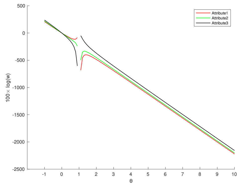
5.2. Discussion of Parameters

In the kernel space, each attribute is automatically given a weight to measure its similarity, and the corresponding subspace is found through feature selection.

$$w_{kd}^{\theta }=\frac{{\left({\sum }_{{\mathit{x}}_{\mathit{i}}\in {\mathit{\pi }}_{\mathit{k}}}exp\left(-\frac{{\sum }_{l\in |O_d|}{\left[I\left(x_{id}=o_{dl}\right)-\frac{{\lambda }_d}{|O_d|}-\left(1-{\lambda }_d\right)f_k\left(o_{dl}\right)\right]}^2}{2{\sigma }^2}\right)\right)}^{\frac{\theta }{1-\theta }}}{{\sum }_{d=1}^D{\left({\sum }_{{\mathit{x}}_{\mathit{i}}\in {\mathit{\pi }}_{\mathit{k}}}exp\left(-\frac{{\sum }_{l\in |O_d|}{\left[I\left(x_{id}=o_{dl}\right)-\frac{{\lambda }_d}{|O_d|}-\left(1-{\lambda }_d\right)f_k\left(o_{dl}\right)\right]}^2}{2{\sigma }^2}\right)\right)}^{\frac{\theta }{1-\theta }}}$$

where $\theta$ is the incentive intensity, and is the allocation parameter of control weight. Figure 1 shows the change in parameters for the weight of the three attributes in the Breastcancer dataset. Here, the discreteness of the three attributes is set to increase from attribute 1. There are four comments for $\theta$.

(1)

When $\theta =0$, $w_{kd}^{\theta }$ is the constant, that is, each attribute will be assigned an equal weight;

(2)

When $\theta =1$, $\frac{\theta }{1-\theta }\to \infty$, but all of the weights must meet the restriction ${\sum }_{d=1}^D{w}_{kd}=1$, so when $\theta \to 1^{+}$, the attribute with the minimum deviation of the sample will be weighted, while the rest of the attributes will be given zero weight; when $\theta \to 1^{-}$, the importance of all attributes tends to be the same;

(3)

When $0<\theta <1$, the more discrete the attribute, the greater its weight;

(4)

When $\theta <0$ and $\theta >1$, the attribute weight is inversely proportional to the dispersion of data distribution. Considering Theorem 1, we should set $\theta >1$, but when $\theta$ is too larger, the difference between attribute weights is reduced.

5.3. Analysis of Synthetic Data and Results

This study used MATLAB (Version 9.9.0.1495850 R2020b) to generate the synthetic data in the experiment. First, four multi-dimensional numerical datasets were generated by the MATLAB function $mvnrnd(·)$, in which the weight of attributes was controlled by setting the variance of attributes, and the correlation degree between attributes was controlled by adjusting the parameters of the covariance matrix. The synthesized numerical data were then discretized by equal width [40] and transformed into categorical data. The synthetic datasets that contain the correct category labels are presented in

Table 1. Data categorized in four synthetic datasets.

	Attributes (D)	Clusters (K)	Samples (N)
Datasets1	6	2	1000
Datasets2	20	2	1000
Datasets3	20	4	1000
Datasets4	40	8	1000

. Four datasets were used to verify the advantages of SKSCC compared with the current mainstream categorical clustering methods.

• The covariance of attribute 1 and attribute 2 is set to −2 in DataSet1, which makes their attributes a negative correlation. The covariance of attribute 1 and attribute 4 is set to 2, which makes their attributes a positive correlation. The variances are set to be equal on each attribute;
• DataSet2 and DataSet1 are set to the same clusters, but the number of attributes differs. Ten attributes are extracted to set their covariance. The variances are set to be equal on each attribute;
• DataSet3 and DataSet2 are set to the same attributes, but the clusters are different. The variances are set to be equal in two clusters. Ten attributes are extracted to set their covariance;
• DataSet4 is set to the most number of attributes and the clusters. Twenty attributes are extracted to set their covariance in seven clusters. All attributes are set to covariance in one cluster. A half clusters set the same variances, as well as other half clusters.

We implemented 100 runs on each algorithm and each dataset, and set $\theta =1.5$. The average clustering accuracy reported in

Table 2. Comparison of F-score and Accuracy results of four algorithms performed on the four synthetic datasets.

Index	Datasets	K-Mode [17]	WKM [22]	MWKM [23]	SKSCC
F-Score	Datasets1	0.9823 ± 0.0000	0.9489 ± 0.0079	0.9738 ± 0.0018	$1.0000\pm 0.0000$
	Datasets2	0.9762 ± 0.0015	0.9860 ± 0.0000	0.9860 ± 0.0000	$0.9940\pm 0.0000$
	Datasets3	0.6346 ± 0.0011	0.5766 ± 0.0018	0.6311 ± 0.0009	$0.6771\pm 0.0005$
	Datasets4	0.5268 ± 0.0008	0.3839 ± 0.0033	0.5367 ± 0.0010	$0.6224\pm 0.0017$
Accuracy	Datasets1	0.9823 ± 0.0000	0.9589 ± 0.0038	0.9746 ± 0.0012	$1.0000\pm 0.0000$
	Datasets2	0.9762 ± 0.0015	0.9860 ± 0.0000	0.9860 ± 0.0000	$0.9939\pm 0.0000$
	Datasets3	0.6755 ±0.0016	0.6037 ± 0.0024	0.6644 ± 0.0009	$0.7033\pm 0.0004$
	Datasets4	0.5863 ± 0.0013	0.5053 ± 0.0147	0.5848 ± 0.0014	$0.6655\pm 0.0014$

reflects the overall performance of each clustering algorithm, and the stability of clustering performance of each algorithm can be judged according to the listed variance. The smaller the variance of clustering accuracy, the better the stability of clustering performance.

From Table 2, we can see that with the increase in the number of related attributes, the clustering accuracy of SKSCC is significantly higher than that of other algorithms. This is because SKSCC employs a “kernel” operation and take into consideration the relationship between attributes.

5.4. Analysis of Real-World Data and Results

In this part of the experiments, we set out to test and verify the performance of SKSCC in real-world datasets. We compared the SKSCC algorithm with three other algorithms: the original k-modes algorithm (k-mode), the weighting algorithm (WKM), and the mixed weighting algorithm (MWKM).

5.4.1. Real-World Datasets

To carry out the experiments, we obtained 10 datasets from the University of California Irvine (UCI) Machine Learning Repository [7].

Table 3. Details of 10 DataSets from UCI.

No.	UCI Datasets	Attributes (D)	Clusters (K)	Samples (N)
1	Breastcancer	9	2	699
2	Vote	16	2	435
3	Mushroom	21	2	8124
4	Adult+stretch	4	2	20
5	Balance	4	3	625
6	Splice	60	3	3190
7	Soybeansmall	35	4	47
8	Car	6	4	1728
9	Dermatology	33	6	366
10	Zoo	15	7	101

lists the details of these 10 datasets. The Breastcancer, Vote, Mushroom, and Adult+stretch datasets have the same clusters, but Mushroom dataset has the most samples, and Adult+stretch dataset has the least number of samples. The Balance and Splice datasets each have the same number of clusters (3), but the dimensionality of Splice is higher. The Soybeansmall and Car datasets each have the same number of clusters (4), but different attributes and samples. Dermatology and Zoo are multi-cluster datasets.

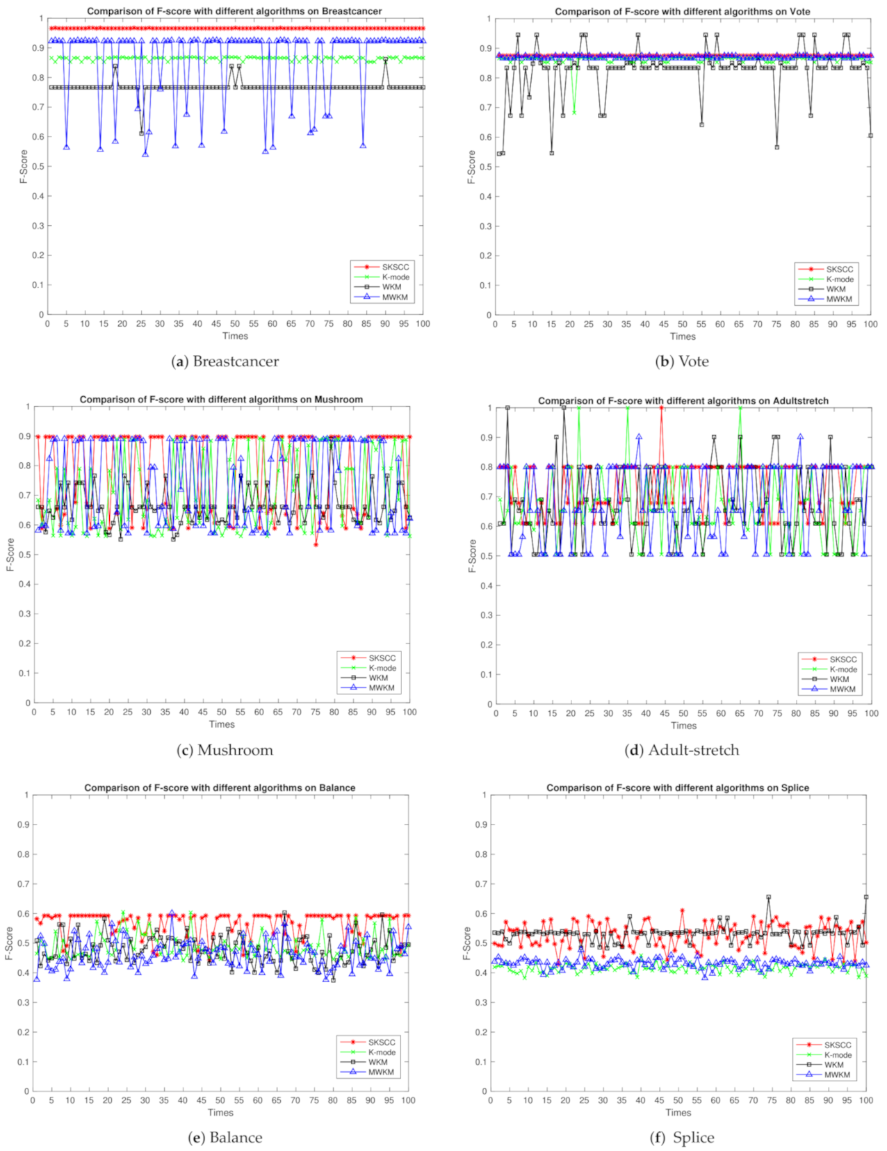
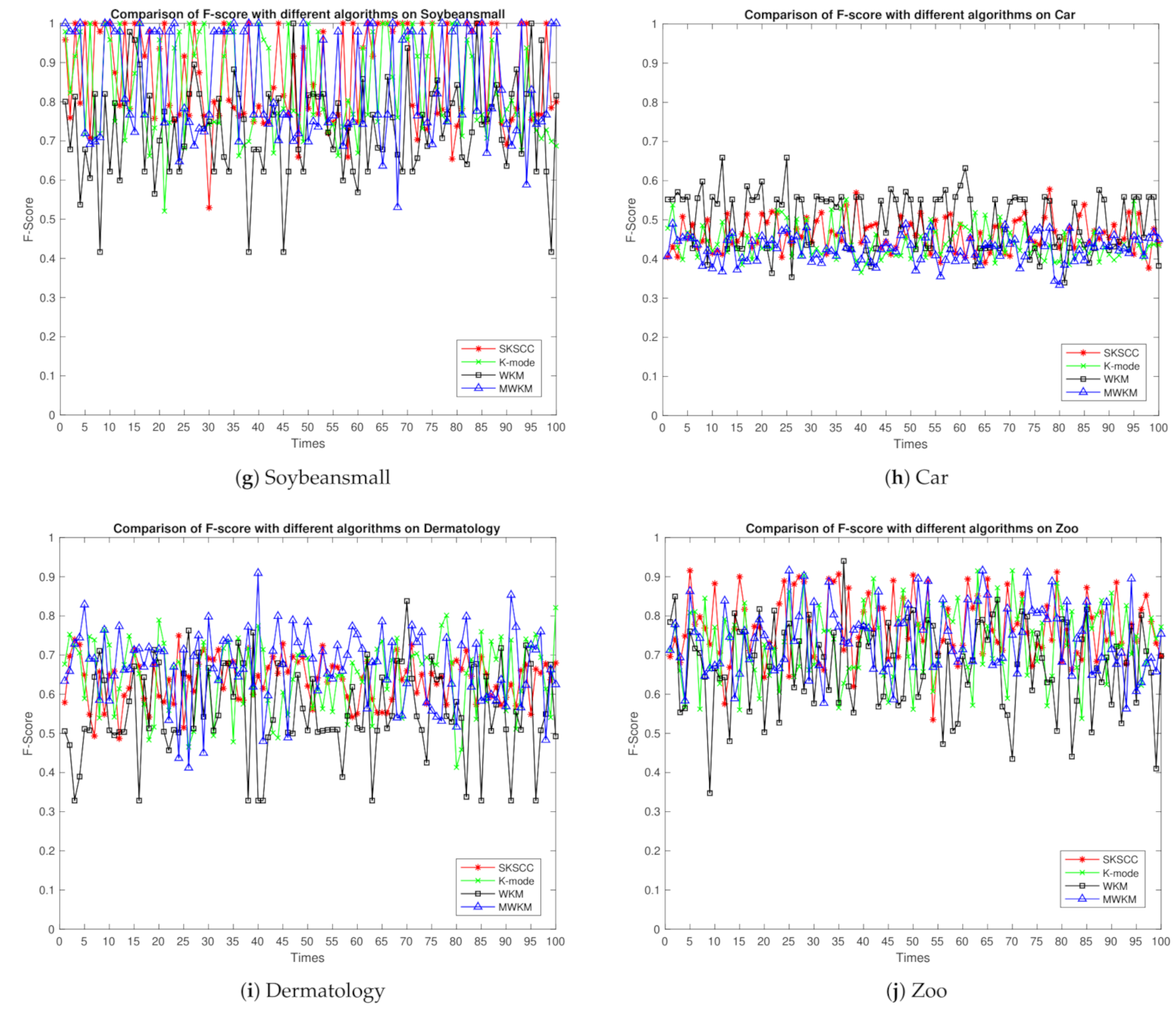
5.4.2. Comparison of Clustering Quality

Because the initial cluster centers can affect the algorithm results, we randomly selected 100 initial centers, and all of the algorithms used the same initial centers in each experiment. We implemented 100 runs on each algorithm and each dataset, and set $\theta =1.5$. The average values and the errors for F-score and accuracy are presented in

Table 4. Comparison of clustering results in terms of F-score and accuracy.

Index	Datasets	K-Mode [17]	WKM [22]	MWKM [23]	SKSCC
F-Score	Breastcancer	0.8637 ± 0.0000	0.7683 ± 0.0005	0.8645 ± 0.0155	$0.9660\pm 0.0000$
	Vote	0.8610 ± 0.0000	0.8238 ± 0.0073	0.8698 ± 0.0000	$0.8749\pm 0.0000$
	Mushroom	0.7159 ± 0.0171	0.6645 ± 0.0034	0.7480 ± 0.0202	$0.7901\pm 0.0193$
	Adult + stretch	0.6691 ± 0.0135	0.6722 ± 0.0159	0.6876 ± 0.0163	$0.7537\pm 0.0085$
	Balance	0.4882 ± 0.0016	0.4782 ± 0.0022	0.4630 ± 0.0024	$0.5672\pm 0.0017$
	Splice	0.4155 ± 0.0000	$0.5321\pm 0.0007$	0.4313 ± 0.0000	$0.5258\pm 0.0019$
	Soybeansmall	0.8324 ± 0.0152	0.7336 ± 0.0157	0.8436 ± 0.0175	$0.8641\pm 0.0146$
	Car	0.4412 ± 0.0018	$0.5006\pm 0.0057$	0.4268 ± 0.0012	0.4738 ± 0.0028
	Dermatology	0.6476 ± 0.0083	0.5573 ± 0.0136	$0.6685\pm 0.0088$	0.6357 ± 0.0034
	Zoo	0.7273 ± 0.0090	0.6716 ± 0.0130	0.7417 ± 0.0074	$0.7701\pm 0.0070$
Accuracy	Breastcancer	0.8621 ± 0.0000	0.8284 ± 0.0000	0.8659 ± 0.0156	$0.9659\pm 0.0000$
	Vote	0.8625 ± 0.0000	0.8244 ± 0.0066	0.8681 ± 0.0000	$0.8734\pm 0.0000$
	Mushroom	0.7536 ± 0.0134	0.8481 ± 0.0157	0.7733 ± 0.0143	0.8194 ± 0.0131
	Adult + stretch	0.7150 ± 0.0160	0.7165 ± 0.0168	0.6910 ± 0.0159	$0.8620\pm 0.0086$
	Balance	0.5251 ± 0.0010	0.4629 ± 0.0033	0.4327 ± 0.0024	$0.8722\pm 0.0321$
	Splice	0.4237 ± 0.0000	$0.6149\pm 0.0011$	0.4314 ± 0.0000	$0.5426\pm 0.0017$
	Soybeansmall	0.8740 ± 0.0110	$0.9423\pm 0.0039$	0.8915 ± 0.0110	0.9085 ± 0.0083
	Car	0.4023 ± 0.0013	$0.4550\pm 0.0095$	0.3593 ± 0.0000	0.4251 ± 0.0038
	Dermatology	0.7085 ± 0.0076	$0.9298\pm 0.0038$	0.7367 ± 0.0063	0.6911 ± 0.0048
	Zoo	0.7937 ± 0.0066	$0.8260\pm 0.0084$	0.7895 ± 0.0073	0.8043 ± 0.0061

. The results showed that our proposed method, SKSCC, achieved the best performance in the comparative experiments on most of the datasets. Because the k-mode [17], WKM [22], and MWKM [23] algorithms are all based on the mode-type category theory, it is easy for them to descend to the clustering objective algorithm’s local minimum, causing them to lose applicability. However, WKM achieved good results on the Car and Splice datasets, while MWKM achieved high accuracy on the Dermatology dataset.

Figure 2 shows the distribution of clustering accuracy for all the algorithms when run 100 times. SKSCC has the best stability. The abscissa represents each algorithm’s running time, and the ordinate is the F-score value to express the results of each clustering. SKSCC has the smallest fluctuation among all the algorithms, although WKM has the best average F-score on the Splice and Car datasets, and MWKM has the best average F-score on the Dermatology dataset. The clustering results for the k-mode algorithms show significant contrast, because they consider only the module in the clustering process, which makes it easy to fall into the local optimum, and the initial cluster center is k randomly selected objects. This is reflected in the standard deviation of average precision. Because SKSCC quantizes the module, it avoids the above-mentioned problems and has more stable performance than the other algorithms.

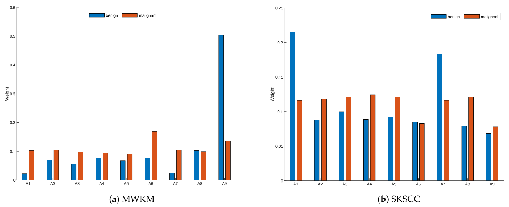
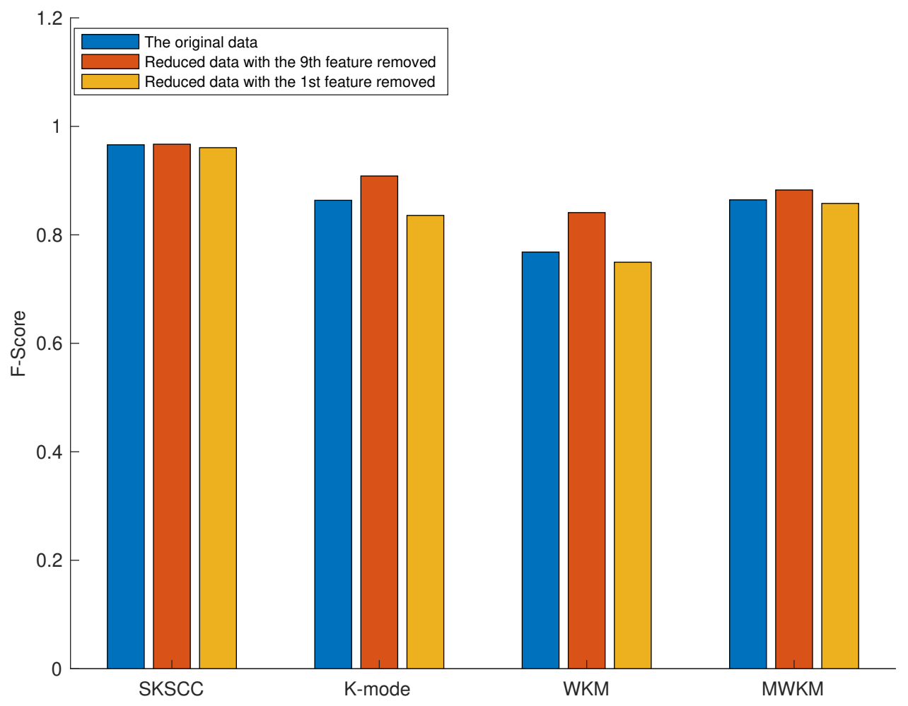
5.4.3. Feature Weighting Results

Our SKSCC approach also has a feature selection effect. Using the Breastcancer dataset as an example, Figure 3 shows the attribute weights generated by the MWKM and SKSCC algorithms. It does not show the k-mode algorithm or WKM algorithm, because the former method is not weighted in its features and the latter method calculates the weights based on mode frequency, which is similar to MWKM algorithm. From Figure 4, we can see that for SKSCC, A1 and A9 acquire the largest and the smallest weights, respectively, of the benign class, but MWKM algorithm achieved the opposite results. To test the feature weighting method’s rationality for the SKSCC, we removed the A1 and A9 features from the original Breastcancer data in order to form two reduced datasets. The F-score values of the different clustering algorithms on the Breastcancer dataset with the original and reduced feature sets are shown in Figure 4. For all the algorithms, the reduced dataset with the A9 feature removed achieved the highest F-score values, while the reduced dataset with the A1 feature removed showed decreased F-score values. The results indicate that our SKSCC algorithm with non-linear similarity measurement does a better job, by considering the relationship of the attributes, than the other algorithms.

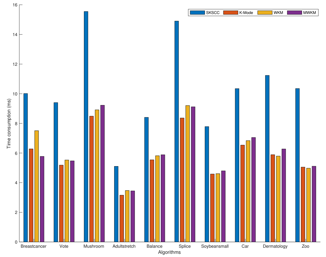
5.4.4. Time Consumption

This paper uses a logarithm of the average time of clustering to compare the actual average times. The ordinate represents the average time (in MS) of each algorithm running on the real-world dataset. It can be seen from Figure 5 that k-mode, WKM, and MWKM algorithms have high clustering efficiency, which is one of the advantages of the module-based clustering algorithms. Because only the module of the categorical attribute needs to be considered, the statistical information of the other categorical symbols can be ignored, which greatly reduces the algorithms’ clustering times.

6. Conclusions

Kernel clustering with categorical data is a vital direction in application research. In view of current problems, such as supposing all features independently, considering all attributes’ importance equally, and finding an optimization solution, this paper proposes a novel kernel clustering approach for categorical data, that is, a self-expressive kernel subspace clustering algorithm for categorical data (SKSCC). This paper first defines a kernel function for self-expression kernel density estimation (SKDE), in which each attribute has its own bandwidth and can be calculated by the data themselves. We also propose a novel non-linear similarity measurement method and an efficient non-linear optimization method (Theorem 1) to solve the objective function of the kernel clustering. Finally, the SKSCC algorithm is presented for categorical data. Our method not only considers the relationship between attributes in non-linear space but also gives each attribute a feature weight to measure the correlation degree in the algorithmic process. The experimental results indicate that the proposed algorithm outperforms the other algorithms on the synthetic and UCI datasets.

There are many directions that are of interest for future exploration. We will expand our approach to other kernel functions and test the performance on more datasets for various data. Our efforts will also be directed at combining our method with deep learning to estimate the parameters adaptively.

References

1. Tang, J.; Liu, H. An unsupervised feature selection framework for social media data. IEEE Trans. Knowl. Data Eng. 2014, 26, 2914–2927. [Google Scholar] [CrossRef] [Green Version]
2. Alelyani, S.; Tang, J.; Liu, H. Feature selection for clustering: A review. Data Clust. Algorithms Appl. 2013, 29, 144. [Google Scholar]
3. Han, J.; Kamber, M. Data Mining: Concepts and Techniques; Morgan Kaufmann: San Francisco, CA, USA, 2001. [Google Scholar]
4. Bharti, K.K.; Singh, P.K. A survey on filter techniques for feature selection in text mining. In Proceedings of the Second International Conference on Soft Computing for Problem Solving (SocProS 2012), Jaipur, India, 28–30 December 2012; Springer: New Delhi, India, 2014; pp. 1545–1559. [Google Scholar]
5. Yasmin, M.; Mohsin, S.; Sharif, M. Intelligent image retrieval techniques: A survey. J. Appl. Res. Technol. 2014, 12, 87–103. [Google Scholar] [CrossRef] [Green Version]
6. Saeys, Y.; Inza, I.; Larranaga, P. A review of feature selection techniques in bioinformatics. Bioinformatics 2007, 23, 2507–2517. [Google Scholar] [CrossRef] [Green Version]
7. Frank, A. UCI Machine Learning Repository. 2010. Available online: http://archive.ics.uci.edu/ml (accessed on 28 March 2021).
8. Jain, A.K.; Murty, M.N.; Flynn, P.J. Data clustering: A review. ACM Comput. Surv. (CSUR) 1999, 31, 264–323. [Google Scholar] [CrossRef]
9. Xu, R.; Wunsch, D. Survey of clustering algorithms. IEEE Trans. Neural Netw. 2005, 16, 645–678. [Google Scholar] [CrossRef] [Green Version]
10. Jain, A.K. Data clustering: 50 years beyond k-mean. Pattern Recognit. Lett. 2010, 31, 651–666. [Google Scholar] [CrossRef]
11. Wu, S.; Lin, J.; Zhang, Z.; Yang, Y. Hesitant fuzzy linguistic agglomerative hierarchical clustering algorithm and its application in judicial practice. Mathematics 2021, 9, 370. [Google Scholar] [CrossRef]
12. Guha, S.; Rastogi, R.; Shim, K. ROCK: A robust clustering algorithm for categorical attributes. Inf. Syst. 2000, 25, 345–366. [Google Scholar] [CrossRef]
13. Andritsos, P.; Tzerpos, V. Information-theoretic software clustering. IEEE Trans. Softw. Eng. 2005, 31, 150–165. [Google Scholar] [CrossRef]
14. Andritsos, P.; Tsaparas, P.; Miller, R.J.; Sevcik, K.C. LIMBO: Scalable clustering of categorical data. In Proceedings of the International Conference on Extending Database Technology, Heraklion, Crete, Greece, 14–18 March 2004; Springer: Berlin/Heidelberg, Germany, 2004; pp. 123–146. [Google Scholar]
15. Qin, H.; Ma, X.; Herawan, T.; Zain, J.M. MGR: An information theory based hierarchical divisive clustering algorithm for categorical data. Knowl.-Based Syst. 2014, 67, 401–411. [Google Scholar] [CrossRef] [Green Version]
16. Xiong, T.; Wang, S.; Mayers, A.; Monga, E. DHCC: Divisive hierarchical clustering of categorical data. Data Min. Knowl. Discov. 2012, 24, 103–135. [Google Scholar] [CrossRef]
17. Huang, Z. Extensions to the k-means algorithm for clustering large data sets with categorical values. Data Min. Knowl. Discov. 1998, 2, 283–304. [Google Scholar] [CrossRef]
18. Huang, Z.; Ng, M.K. A fuzzy k-modes algorithm for clustering categorical data. IEEE Trans. Fuzzy Syst. 1999, 7, 446–452. [Google Scholar] [CrossRef] [Green Version]
19. Ng, M.K.; Li, M.J.; Huang, J.Z.; He, Z. On the impact of dissimilarity measure in k-modes clustering algorithm. IEEE Trans. Pattern Anal. Mach. Intell. 2007, 29, 503–507. [Google Scholar] [CrossRef] [PubMed]
20. Bai, L.; Liang, J.; Dang, C.; Cao, F. The impact of cluster representatives on the convergence of the k-modes type clustering. IEEE Trans. Pattern Anal. Mach. Intell. 2012, 35, 1509–1522. [Google Scholar] [CrossRef] [PubMed]
21. Cao, F.; Liang, J.; Li, D.; Zhao, X. A weighting k-modes algorithm for subspace clustering of categorical data. Neurocomputing 2013, 108, 23–30. [Google Scholar] [CrossRef]
22. Chan, E.Y.; Ching, W.K.; Ng, M.K.; Huang, J.Z. An optimization algorithm for clustering using weighted dissimilarity measures. Pattern Recognit. 2004, 37, 943–952. [Google Scholar] [CrossRef]
23. Bai, L.; Liang, J.; Dang, C.; Cao, F. A novel attribute weighting algorithm for clustering high-dimensional categorical data. Pattern Recognit. 2011, 44, 2843–2861. [Google Scholar] [CrossRef]
24. Chen, L.; Wang, S.; Wang, K.; Zhu, J. Soft subspace clustering of categorical data with probabilistic distance. Pattern Recognit. 2016, 51, 322–332. [Google Scholar] [CrossRef]
25. Han, J.; Kamber, M.; Pei, J. Data mining concepts and techniques third edition. Morgan Kaufmann Ser. Data Manag. Syst. 2011, 5, 83–124. [Google Scholar]
26. Guyon, I.; Elisseeff, A. An introduction to variable and feature selection. J. Mach. Learn. Res. 2003, 3, 1157–1182. [Google Scholar]
27. Breiman, L.; Friedman, J.; Stone, C.J.; Olshen, R.A. Classification and Regression Trees; CRC Press: Boca Raton, FL, USA, 1984. [Google Scholar]
28. Kohavi, R.; John, G.H. Wrappers for feature subset selection. Artif. Intell. 1997, 97, 273–324. [Google Scholar] [CrossRef] [Green Version]
29. Pashaei, E.; Aydin, N. Binary black hole algorithm for feature selection and classification on biological data. Appl. Soft Comput. 2017, 56, 94–106. [Google Scholar] [CrossRef]
30. Rasool, A.; Tao, R.; Kamyab, M.; Hayat, S. Gawa—A feature selection method for hybrid sentiment classification. IEEE Access 2020, 8, 191850–191861. [Google Scholar] [CrossRef]
31. Liu, H.; Setiono, R. Chi2: Feature selection and discretization of numeric attributes. In Proceedings of the 7th IEEE International Conference on Tools with Artificial Intelligence, Herndon, VA, USA, 5–8 November 1995; pp. 388–391. [Google Scholar]
32. Quinlan, J.R. Induction of decision trees. Mach. Learn. 1986, 1, 81–106. [Google Scholar] [CrossRef] [Green Version]
33. Quinlan, J.R. C4. 5: Programs for Machine Learning; Elsevier: Amsterdam, The Netherlands, 2014. [Google Scholar]
34. Kandaswamy, K.K.; Pugalenthi, G.; Hazrati, M.K.; Kalies, K.U.; Martinetz, T. BLProt: Prediction of bioluminescent proteins based on support vector machine and relieff feature selection. BMC Bioinform. 2011, 12, 345. [Google Scholar] [CrossRef] [PubMed] [Green Version]
35. Shao, J.; Liu, X.; He, W. Kernel based data-adaptive support vector machines for multi-class classification. Mathematics 2021, 9, 936. [Google Scholar] [CrossRef]
36. Robnik-Šikonja, M.; Kononenko, I. Theoretical and empirical analysis of ReliefF and RReliefF. Mach. Learn. 2003, 53, 23–69. [Google Scholar] [CrossRef] [Green Version]
37. Le, T.T.; Urbanowicz, R.J.; Moore, J.H.; McKinney, B.A. Statistical inference Relief (STIR) feature selection. Bioinformatics 2019, 35, 1358–1365. [Google Scholar] [CrossRef]
38. Huang, Z.; Yang, C.; Zhou, X.; Huang, T. A hybrid feature selection method based on binary state transition algorithm and ReliefF. IEEE J. Biomed. Health Inform. 2018, 23, 1888–1898. [Google Scholar] [CrossRef] [PubMed]
39. Deng, Z.; Chung, F.L.; Wang, S. Robust relief-feature weighting, margin maximization, and fuzzy optimization. IEEE Trans. Fuzzy Syst. 2010, 18, 726–744. [Google Scholar] [CrossRef]
40. Chen, L.F. A probabilistic framework for optimizing projected clusters with categorical attributes. Sci. China Inf. Sci. 2015, 58, 1–15. [Google Scholar] [CrossRef]
41. Kong, R.; Zhang, G.; Shi, Z.; Guo, L. Kernel-based k-means clustering. Comput. Eng. 2004, 30, 12–14. [Google Scholar]
42. Elhamifar, E.; Vidal, R. Sparse subspace clustering: Algorithm, theory, and applications. IEEE Trans. Pattern Anal. Mach. Intell. 2013, 35, 2765–2781. [Google Scholar] [CrossRef] [Green Version]
43. Ji, P.; Zhang, T.; Li, H.; Salzmann, M.; Reid, I. Deep subspace clustering networks. arXiv 2017, arXiv:1709.02508. [Google Scholar]
44. You, C.; Li, C.G.; Robinson, D.P.; Vidal, R. Oracle based active set algorithm for scalable elastic net subspace clustering. In Proceedings of the IEEE Conference on Computer Vision and Pattern Recognition, Las Vegas, NV, USA, 26 June–1 July 2016; pp. 3928–3937. [Google Scholar]
45. Chen, L.; Guo, G.; Wang, S.; Kong, X. Kernel learning method for distance-based classification of categorical data. In Proceedings of the 2014 14th UK Workshop on Computational Intelligence (UKCI), Bradford, UK, 8–10 September 2014; pp. 1–7. [Google Scholar]
46. Ouyang, D.; Li, Q.; Racine, J. Cross-validation and the estimation of probability distributions with categorical data. J. Nonparametr. Stat. 2006, 18, 69–100. [Google Scholar] [CrossRef]
47. Huang, Z. Clustering large data sets with mixed numeric and categorical values. In Proceedings of the 1st Pacific-Asia Conference on Knowledge Discovery and Data Mining (PAKDD), Singapore, 23–24 February 1997; pp. 21–34. [Google Scholar]
48. Cheung, Y.M.; Jia, H. Categorical-and-numerical-attribute data clustering based on a unified similarity metric without knowing cluster number. Pattern Recognit. 2013, 46, 2228–2238. [Google Scholar] [CrossRef]
49. Zhong, S.; Chen, D.; Xu, Q.; Chen, T. Optimizing the gaussian kernel function with the formulated kernel target alignment criterion for two-class pattern classification. Pattern Recognit. 2013, 46, 2045–2054. [Google Scholar] [CrossRef]
Figure 1. Analysis of weight with different θ .
Mathematics 09 01680 g001
Figure 2. Comparison of F-score with different algorithms on different datasets.
Mathematics 09 01680 g002aMathematics 09 01680 g002b
Figure 3. Weight distributions generated by two algorithms on Breastcancer dataset.
Mathematics 09 01680 g003
Figure 4. F-score values of the different clustering algorithms on the Breastcancer dataset with original and reduced feature sets.
Mathematics 09 01680 g004
Figure 5. F-Score values of the different clustering algorithms on the Breastcancer dataset with original and reduced feature sets.
Mathematics 09 01680 g005