Stochastic Analysis of the Time Continuum ^†

Abstract

This paper considers the time continuum of Brouwer in terms of the complex system physics. It is based upon a processual definition of real numbers which concern the measurement problem. The multiresolution hierarchy of the measurement process is represented by the time operator acting on continuous signals. The wavelet domain hidden Markov model, which recapitulates statistical properties of the hierarchy, is verified experimentally on a wide range of signal ensembles. It indicates a novel method that has already been proved to be tremendously useful in applied mathematics.

1. Introduction

Chaitin has announced the decline and fall of reductionism in mathematics, considering the randomness in arithmetic elucidated by some results of the computation theory. The concluding remark concerns experimental mathematics in order to stress the impact of computers that have an enormous contribution to the mathematical experience, which impels people to proceed in a more pragmatic fashion. Mathematicians are coerced to go ahead proof, postulating hypotheses based upon results of computer experiments. He particularly points out a relation to the contemporary physics wherein randomness is a crucial agent, which is regarded to be the core of an emergent science paradigm. Chaitin finally remarked that the question of how one should actually do mathematics requires at least another generation of work [1] (pp. 156–159).

Randomness that emerges in a formal theory set upon deterministic assumptions concerns the complex system physics, which considers systems wherein the best method of description is not clear a priori [2] (p. 203). The statistical complexity suggested by Grassberger [3], which corresponds to stochastic computing in terms of the Bernoulli–Turing machine, is analogous to the deterministic one designed on the Turing machine [4]. Within the stochastic computation theory, deterministic and random behaviors are regarded to be elemental extremes deprived of a vital component since they both share a common failure to support emergent properties. Being the amalgam of both, complex patterns have an inherent tendency towards hierarchical organization [2] (p. 200).

Such a hierarchy has substantial implications concerning cognition, since observation and intellection are related to the neural architecture whose structure is reflected by cognitive complexity [2] (pp. 204–206). It corresponds to the evolution in a hierarchical manner [5] (pp. 470–477), indicating the concept of time that operates not only physically or biologically but also in terms of organization theory. In this regard, time corresponds to a primordial intuition which is the very base of conscious life—as stated by Brouwer‘s intention to establish the continuum upon such intuitionism [6] (pp. 36–45). Intuitionistic mathematics is considered to be the intellection of increasingly complex features, which is related to self-organization of complex systems due to the definition that originates from Shalizi concerning the increase in complexity over time [7]. The issue requires formulation of the complex system physics based upon the time operator acting on the space of continuous signals, which is actually a straightforward generalization of a multiresolution hierarchy that relates the measurement process [8] (p. 107).

The paper is intended to elucidate the intuitionistic mathematics in terms of complex systems. The next section briefly outlines the intuitionism by Brouwer and suggests the time operator formulation of the complex system physics, which was developed by the Brussels school of thermodynamics. The third section concerns the continuum structure presenting a processual definition of real numbers corresponding to the measurement. In order to consider the time operator of a multiresolution hierarchy, the concept of a signal ensemble was derived in analogy to the quantum theory one. The fourth section elaborates on results in regard to a signal processing model that recapitulates statistical properties of the hierarchy, which is obtained by experimental mathematics methods. The last section contains concluding remarks.

The article contents have mostly been published in the form of a conference paper by M.M. and S.V. [9]. The main advancement corresponds to the discussion of the measurement problem, wherein some corroborations of the statistical model are presented. Proofs are indicated using the theory of quantum ensembles, which has not appeared in relation to the signal processing so far. The paper also contains an elaboration of the measurement process in terms of the signal space and its dual, which is seldom encountered in the literature. Novel illustrations have been added as well in order to make the article more comprehensible.

2. Materials and Methods

2.1. The Intuitionistic Mathematics

Brouwer’s contribution to mathematics foundations concerns the context of the XIX and the XX centuries, whose eminent personalities were Hilbert, Russell and Whitehead. Russell and Whitehead‘s view was based upon the statement that logic represents the fundament of mathematical thought as Hilbert stated that a formal language was the design of mathematics. Brouwer referred to both viewpoints as platonic ones, since they use timeless conceptions which make them deterministic theories.

He advocated irreducibility of mathematics to a language, in aim to separate it from formalism and logicism as well [10]. In his opinion, the base of consciousness is the time continuum transcending any language in order to provide the original creation. It represents a continual activity of the creative subject that is not formally determined, which means that for mathematics there is no certain language [11]. He used the term choice sequence, also separating intuitionism from constructive mathematics based upon deterministic decisions [6] (pp. 38–40).

Considering the intuitionistic logic, one discerns its deviation from formal laws of the excluded middle and of the double negation. Brouwer regarded a structure to be discrete if the law of excluded middle $x=y\vee x\ne y$ holds, which is not generally true [12]. Intuitionism is actually a logic of continuum, unlike the formal logic that is a discrete one. The double negation law $\neg x\ne y\Rightarrow x=y$ is also violated, which makes the existence of infinitesimals possible since the negation of diversity from zero $\neg ϵ\ne 0$ is not reduced to the identity $ϵ=0$ [13]. The continuum in such a regard does not reduce to a pointwise set, which means that the primordial intuition is not dependent on a formal spatiality. However, the sense of time has been seriously damaged by treating it as an additional dimension of the formal space that modern science peddles for an ultimate reality [6] (pp. 36–37).

Brouwer actually refers to the elimination of time stated by Meyerson due to his definition of modern science in terms of progressively realizing the fundamental bias in human reasoning, which concerns the reduction of difference and change onto identity and constancy [14]. As early as 1754, d‘Alambert noted that one should consider duration as a fourth dimension supplementing the common three-dimensional design [15] and Lagrange went so far to term it the four-dimensional geometry [16] (p. 223). Such a historical trail reached its climax in Einstein, who was categorically rejecting the existence of change, considered by him to be a mere illusion [17] (pp. 201–203). Einstein‘s intension to reach the timeless world of supreme rationality was definitely manifested in the celebrated Einstein–Bohr debate on the foundations of quantum theory. The core of the debate concerned the fundamental role of randomness in specifying a system‘s state, which was emphatically denied by Einstein who was supporting an objective epistemology of science. Although he overturned Newtonian mechanics, Einstein firmly held the Cartesian view of reducing physics to geometry in terms of the formal spatiality that was but a deterministic assumption. In that respect, contemporary restoration of time indicates postmodernism in science, whose forerunner has been Brouwer [6] (p. 49).

2.2. The Time Operator

The occurrence of postmodern science is related to quantum theory, whose origin dates back to the beginning of the XX century [18]. The statistical formulation concerning the evolution of probabilities has given rise to the operator mechanics by Koopman and von Neumann, in which a system corresponds to the evolutionary group of transformations $U^t$ acting on the Hilbert space $L_{\mu }^2(\Omega )$. Considering that the transformation is induced by pointwise dynamics $X^t:\Omega \to \Omega$, which preserves the probability measure $\mu$ in the phase space $\Omega$, the operator $U^t=X^t\circ ·$ should be unitary and, according to the Stone theorem, the group has an infinitesimal generator termed the Liouvillian L [19].

The uncertainty principle concerns a pair of complementary observables, which consist of the position $Q=q·$ and the momentum operator $P=\frac{\partial ·}{i\partial q}$. Formulated in terms of the commutator $[Q,P]=QP-PQ$, the uncertainty implies relation $[Q,P]=iI$. In the same manner, the time operator T is defined to satisfy the uncertainty relation

$$\begin{array}{c}\hfill [T,L]=iI\end{array}$$

(1)

concerning the Liouvillian L [17].

The variable F, whose domain is $\Omega$, evolves by action of the group $U^t=e^{-iLt}$, whilst the distribution density $\rho$ is governed by its adjoints $U^{t†}=e^{iLt}$, which implies the Liouville equation $\frac{\partial \rho }{i\partial t}=L\rho$. Consequently, the Liouvillian L and the time operator T correspond to complementary observables in analogy to the position and the momentum in quantum theory. In terms of the group action, the relation (1) is equivalent to

$$\begin{array}{c}\hfill [T,U^t]=t{U}^t\end{array}$$

(2)

which comes down to $[T,U]=U$, supposing the cyclic group generated by $U\equiv U^1$.

The time operator existence in the system induces a change in representation $\Lambda =\lambda \left(T\right)$, transfiguring, with no loss of information, the group to a semigroup action [20]. The semigroup

$$\begin{array}{c}\hfill W^{t†}=\Lambda U^{t†}{\Lambda }^{-1},t\ge 0\end{array}$$

(3)

corresponds to an irreversible evolution of the complex system, conjugated to the reversible one of the group. It addresses a stochastic process that is irreducible to deterministic description, whose existence is analogous to the Gödel theorem concerning an incompleteness of the arithmetic [21].

In modern science, based upon the elimination of time, irreversibility is cognized through the measurement problem that demands a departure from determinism in favor of statistical causality [17] (pp. 65–67). Quantum measurement corresponds to a reduction in the distribution density, which is a nonunitary transformation. Von Neumann expressed its difference from the unitary evolution by the Liouville equation in terms of the entropy increase, invoking a substantial role of the observer [22] (pp. 347–416). Irreversibility therefore appears to be at the very core of physics.

3. Results

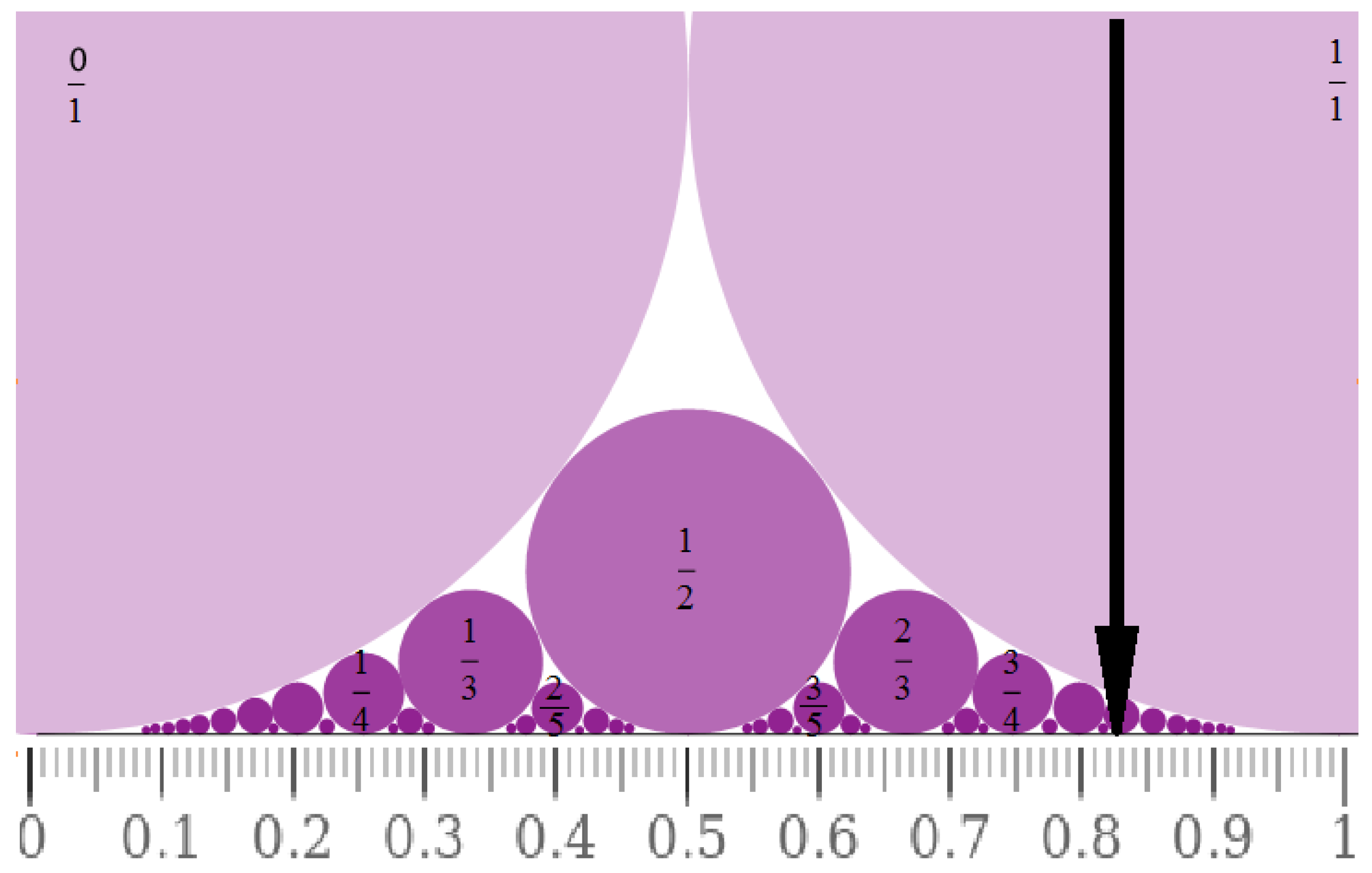
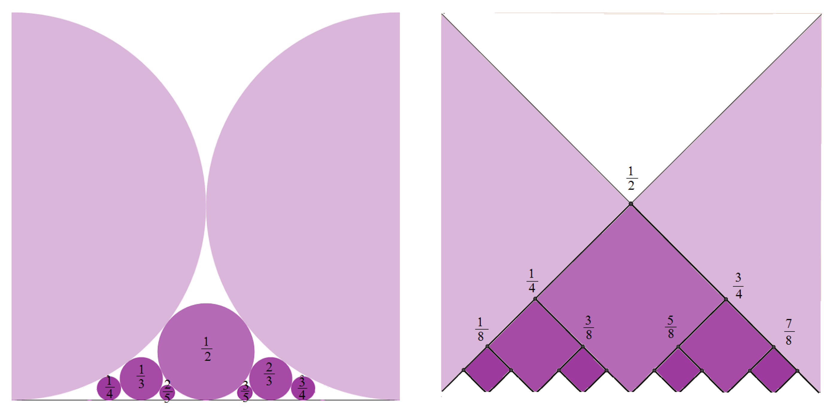
3.1. The Continuum of Reals

3.1.1. Real Numbers

The concept of continuum corresponds to real numbers which designate the measurement process originating from Euclide’s geometrical algebra. In the V book of the Elements, he elaborates on the doctrine of proportion, which concerns commensuration of magnitudes. According to the Euclidean algorithm, magnitudes a and b measure each other through

$$\begin{array}{c}\hfill \frac{a}{b}=\frac{1}{n_1+\frac{1}{n_2+\frac{1}{\ddots }}}\end{array}$$

(4)

which is termed the continued fraction, having the spectrum $n_1,n_2,\dots$ One assumes that $a\le b$, i.e., $a/b\le 1$. The proportion $\frac{a}{b}=\frac{c}{d}$, which is indicated by matching of the respective terms in both spectra, induces identity on the continuum of reals. Consequently, a real number corresponds to the fraction expansion (4), implying a measurement process that takes place step by step over time (Figure 1).

The time evolution is represented by the Ford diagram of circles [23], whose intersections with a vertical line correspond to the sequence

$$\begin{array}{c}\hfill {\xi }_i=\frac{1}{n_1+\frac{1}{\ddots +\frac{1}{n_i}}}\end{array}$$

(5)

identifying a real number x (Figure 2). The element ${\xi }_i=\frac{h_i}{k_i}$ is termed the Diophantine approximation, being the most approximate to the real number x in regard to fractions $\frac{h}{k}$, $k\le k_i$ whose denominators are not greater than one of ${\xi }_i$. Denominators and numerators of the sequence are obtained by the recurrence equations

$$\begin{array}{c}\hfill h_{i+1}=n_{i+1}{h}_i+h_{i-1},k_{i+1}=n_{i+1}{k}_i+k_{i-1}\end{array}$$

(6)

considering the initial conditions $h_0=0$, $h_1=1$ and $k_0=1$, $k_1=n_1$. The difference of successive members is

$$\begin{array}{c}\hfill \Delta {\xi }_i={\xi }_{i+1}-{\xi }_i=\frac{h_{i+1}}{k_{i+1}}-\frac{h_i}{k_i}=\frac{h_{i+1}{k}_i-h_i{k}_{i+1}}{k_{i+1}{k}_i}=\frac{⟦h,{k⟧}_i}{k_{i+1}{k}_i}\end{array}$$

(7)

supposing $⟦h,{k⟧}_i=h_{i+1}{k}_i-h_i{k}_{i+1}$, which implies

$$\begin{array}{c}\hfill ⟦h,{k⟧}_i=(a_{i+1}{h}_i+h_{i-1})k_i-h_i(a_{i+1}{k}_i+k_{i-1})=h_{i-1}{k}_i-h_i{k}_{i-1}=-{⟦h,k⟧}_{i-1}\end{array}$$

(8)

and keeping in mind $⟦h,{k⟧}_0=h_1{k}_0-h_0{k}_1=1$, one obtains $⟦h,{k⟧}_i={(-1)}^i$, i.e.,

$$\begin{array}{c}\hfill \Delta {\xi }_i=\frac{{(-1)}^i}{k_i{k}_{i+1}}\end{array}$$

(9)

In this respect, the continued fraction concerning a real number takes the form of an alternating series

$$\begin{array}{c}\hfill x=\Delta {\xi }_0+\dots +{\xi }_i+\dots =\frac{1}{k_0{k}_1}-\dots \frac{{(-1)}^i}{k_i{k}_{i+1}}\dots \end{array}$$

(10)

which is a sparse representation [24] composed of terms from the redundant dictionary $\frac{1}{1},\frac{1}{2},\frac{1}{3}\dots$.

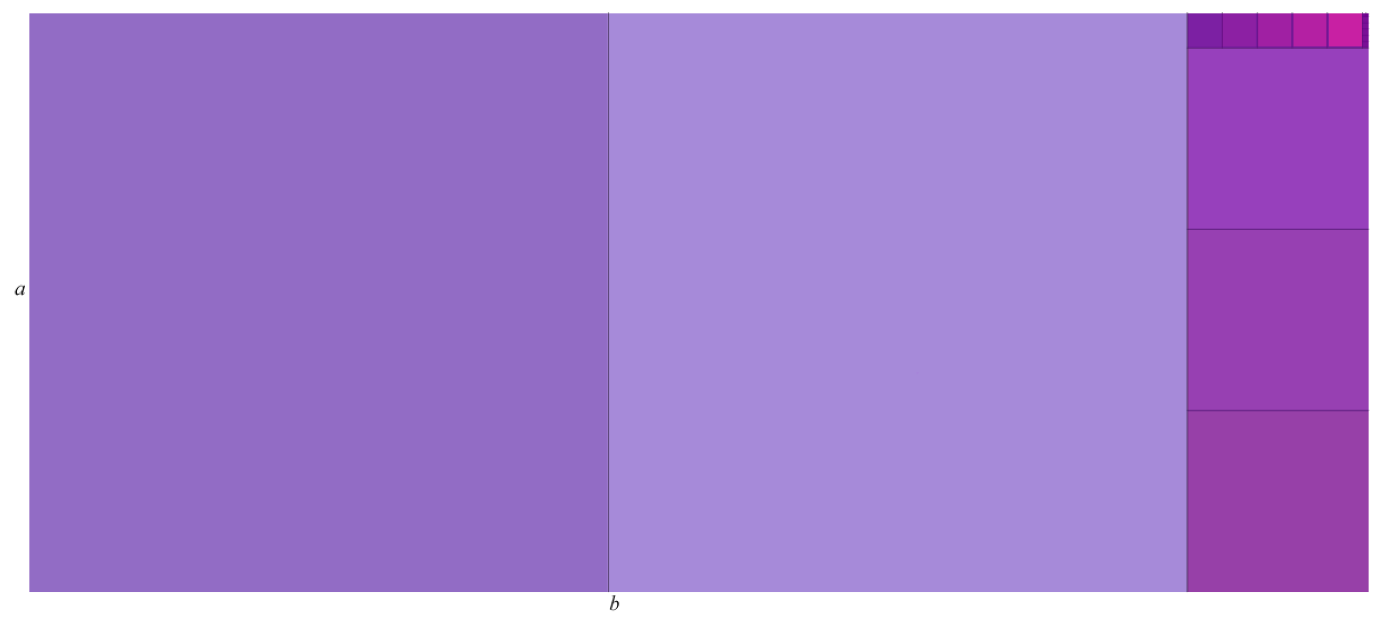
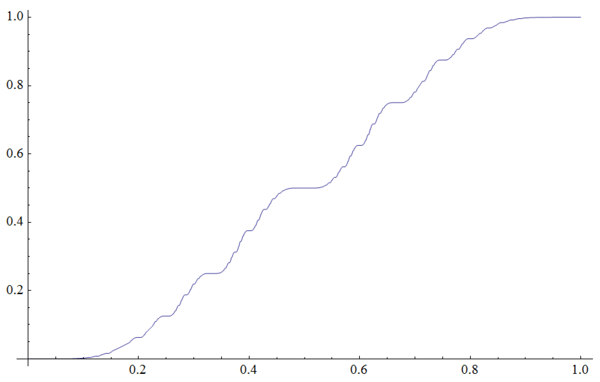
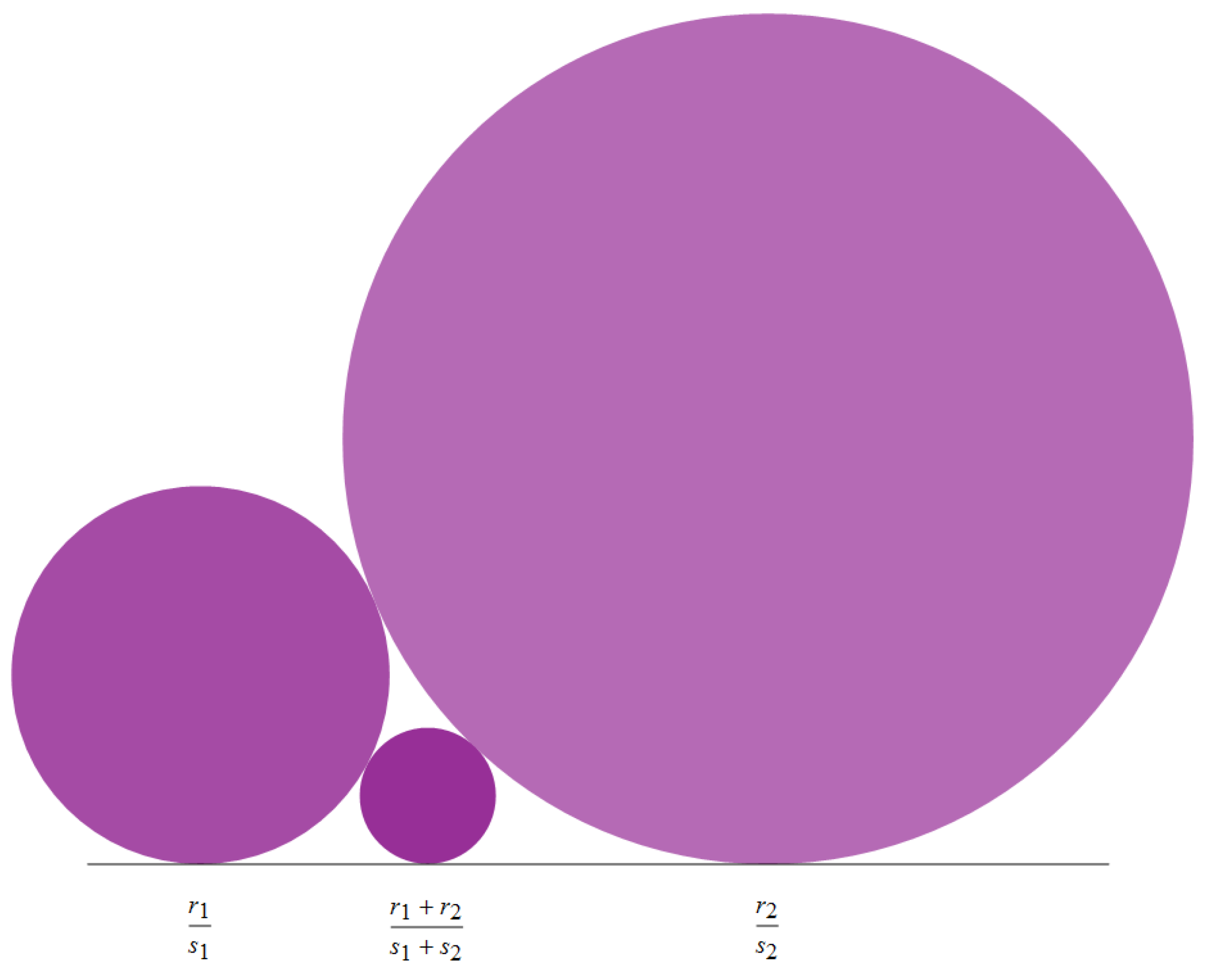
3.1.2. The Continuum Structure

Equation (10) corresponds to a binary code wherein 0 is assigned to the terms of the dictionary that do not participate in the series and 1 to those that do participate, preceded by an alternating ± sign. Such a representation of the real number is highly redundant since the entire dictionary cannot be involved in a series. One should therefore eliminate excess zeros, which is achieved by coding the spectrum $n_1,n_2,\dots$ A binary code like this is composed of alternative ± values different from zero at positions $n_1,n_1+n_2,\dots$, which gives rise to the Minkowski question mark function (Figure 3).

$$\begin{array}{c}\hfill ?:\frac{1}{n_1+\frac{1}{n_2+\frac{1}{\ddots }}}\mapsto \frac{1}{2^{n_1-1}}-\frac{1}{2^{n_1+n_2-1}}+\dots \end{array}$$

(11)

that is a procedure transfiguring the continued fraction to the binary code. It represents an automorphism of the continuum, mapping the real number $x=\frac{1}{n_1+\frac{1}{n_2+\frac{1}{\ddots }}}$ to an analog value $?\left(x\right)={\sum }_i^{}\frac{{(-1)}^{i-1}}{2^{n_1+\dots +n_i-1}}$. Under the term continuum, one assumes the skeletal category that is specified up to an isomorphism. The transformation ? is therefore considered to be an automorphism of the structure, since an isomorphism (12) hereinafter is also the identity.

The Ford diagram is structured by the hierarchy of scales, each one corresponding to the insertion of circles tangent to two of them at the previous scales, as well as to the number line (Figure 4). In such a hierarchy, each circle is attributed to an irreducible fraction that represents its contact with the line.

If designators of two circles are $\frac{r_1}{s_1}$ and $\frac{r_2}{s_2}$, the inserted circle between them corresponds to the fraction $\frac{r_1+r_2}{s_1+s_2}$. One denotes it as $\frac{r_1}{s_1}\oplus \frac{r_2}{s_2}$, which is an operation termed the mediant or the Farey sum. It is due to John Farey, who noticed that successive fractions $\zeta <\xi <\eta$, whose denominators in the reduced form are up to a given value, relate by $\xi =\zeta \oplus \eta$. For instance, the fractions up to the denominator value 5 form the order $0/1,1/5,1/4,1/3,2/5,1/2,3/5,2/3,3/4,4/5,1/1$, where each successive threesome is related by the Farey sum [25].

The question mark function maps the mediant to the arithmetic mean [26]

$$\begin{array}{c}\hfill ?(x\oplus y)=\frac{?\left(x\right)+?\left(y\right)}{2}\end{array}$$

(12)

which is an isomorphism of topological quasigroups, whose action turns circles of the Ford diagram into square-like diamonds (Figure 5). Such a diagram has the binary tree structure wherein nodes, coordinated by $x=\frac{2k-1}{2^{j+1}}$ and $y=\frac{1}{2^{j+1}}$, correspond to paracomplex numbers $x+ıy$, ${ı}^2=1$ [27] that form the algebra of segments $[x-y,x+y]$. Branching of segments $[\frac{k-1}{2^j},\frac{k}{2^j}],1\le k\le 2^j$ designates binary digits of the real number and, in this regard, the hierarchy of the continuum is related to such a binary coding. The Rényi map

$$\begin{array}{c}\hfill R\left(x\right)=\left\{\begin{array}{cc}2x,& 0\le x<\frac{1}{2}\\ 2x-1,& \frac{1}{2}<x\le 1\end{array}\right.\end{array}$$

(13)

that concerns a shift in terms of binary digits is a self-similarity of the structure, mapping both the left and right subtrees to the entire one.

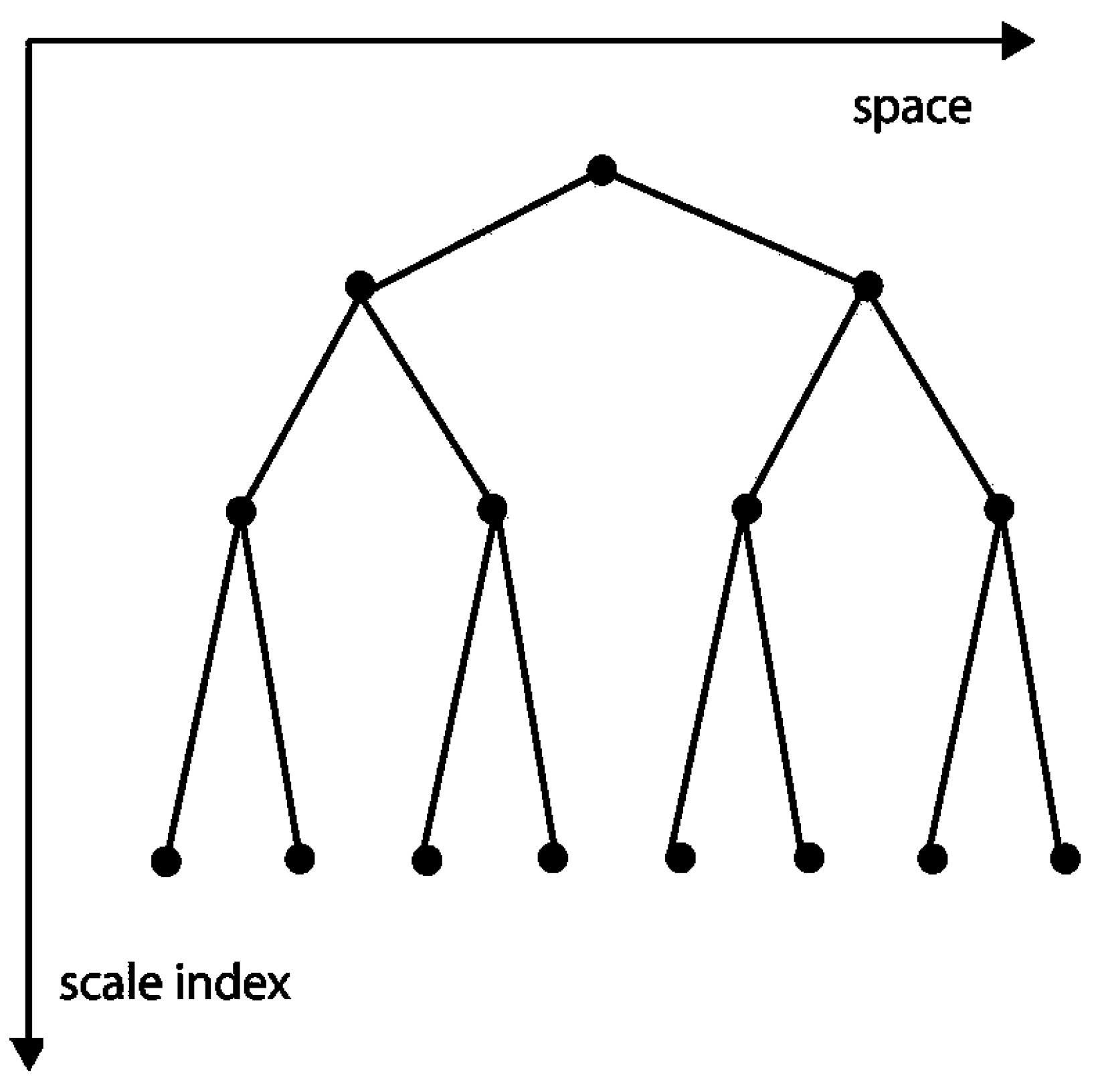
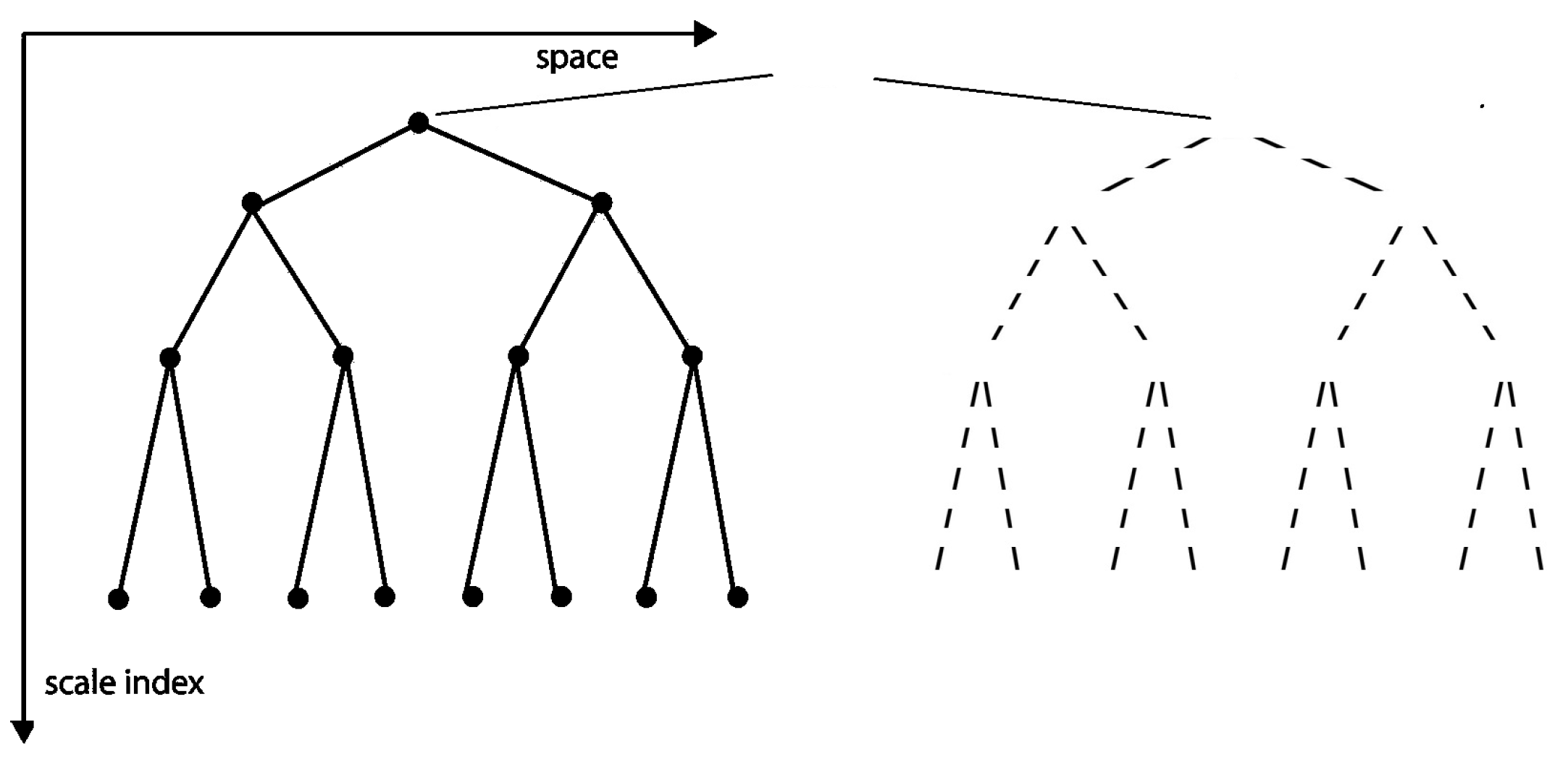
3.2. Wavelets and Multiresolution Hierarchy

3.2.1. The Signal Space

In order to regard the measurement process in terms of the time operator, one requires the space of continuous signals that should be discussed in a dual manner. If one considers the measurement states $\Sigma$, a dual space ${\Sigma }^{\prime }=\Delta$ corresponds to the devices evaluating them. If one, on the other hand, considers the measurement devices $\Delta$, states appear in the form of a dual space ${\Delta }^{\prime }=\Sigma$. These options may differ in more than a conceptual sense: taking the dual of the dual does not necessarily bring back to the departure. Even if it does, there may be some reasons to favor one over the other since an aspect of the continuum structure is obscured [28] (pp. 16–23).

The intention presented in the paper considers continuous signals to be both states and devices concurrently, which should lead to a source–detector interchangeability, termed crossing in quantum theory [28] (p. 20). This is a reason the signal space is an autodual one $\Sigma =\Delta =L^2\left(\mathbb{I}\right)$, emphasizing the Lebesgue measure on the domain $\mathbb{I}=[0,1]$. The topology of the Hilbert space $L^2\left(\mathbb{I}\right)$ is not a trivial issue, since it is governed by equality that tolerates continuous signals to differ in zero measured domains. Such an occasion makes it possible to establish the norm $\parallel ·\parallel$ and the scalar product $\langle ·|·\rangle$ playing an essential role in autoduality.

The continuum structure is reflected by wavelet bases of $L^2\left(\mathbb{I}\right)$, which are hierarchically indexed according to nodes of the binary tree. The signal decomposition considering a wavelet base takes place in the representational form

$$\begin{array}{c}\hfill A_0+\sum _{j\ge 0}^{}\sum _{k=1}^{2^j}{D}_{j,k}{\psi }_{j,k}\end{array}$$

(14)

whereat $A_0$ is the approximate coefficient and $D_{j,k}$ are detail coefficients that corresponds to tree nodes [29] (pp. 304–307). The Haar base is paradigmatically designed by translations and normalized dilatations of the mother wavelet $\chi \left(x\right)=\left\{\begin{array}{cc}-1,& 0\le x<\frac{1}{2}\\ +1,& \frac{1}{2}<x<1\end{array}\right.$ in the manner of

$$\begin{array}{c}\hfill {\chi }_{j,k}\left(x\right)=\left\{\begin{array}{cc}-2^{j/2},& \frac{k}{2^j}\le x<\frac{k+1/2}{2^j}\\ +2^{j/2},& \frac{k+1/2}{2^j}<x\le \frac{k+1}{2^j}\end{array}\right.\end{array}$$

(15)

meaning that the basic elements have a value of zero elsewhere.

A wavelet base is also interpreted in a dual manner concerning states and devices of the measurement process. It corresponds to a distribution density, which implies the unit norm $\parallel {\psi }_{j,k}\parallel =1$. A variable $X_{j,k}$, which is distributed according to the density $|{\psi }_{j,k}{|}^2$, has the expectation value $E{X}_{j,k}=\frac{2k-1}{2^{j+1}}$, which is actually the spatial position of a tree node. On the other hand, it consists of variables ${\psi }_{j,k}$ that are mutually independent since $(j,k)\ne (l,m)\Rightarrow E{\psi }_{j,k}{\psi }_{l,m}=E{\psi }_{j,k}E{\psi }_{l,m}=0$, which means orthogonality $\langle {\psi }_{j,k}|{\psi }_{l,m}\rangle ={\delta }_{(j,k)}^{(l,m)}$. Moreover, their expectations are zero and they are equally distributed within each scale. Such an interpretation of the wavelet base represents measurement devices $\Delta$ which are modelled due to hierarchical structuring. In that respect, measurement states are represented by detail coefficients $D_{j,k}=\langle {\psi }_{j,k}|·\rangle$ and the approximation coefficient $A_0=\langle 1|·\rangle$, which form a base of the dual space $\Sigma ={\Delta }^{\prime }$.

The hierarchical structure of a wavelet base is reflected in detail coefficients, which means that each of them at a scale j of the binary tree has two successors at the next one $j+1$ (Figure 6). The succession is related to the measurement process whose steps correspond to scales of the hierarchy. In that respect, the time concerning a wavelet base is presented by the operator

$$\begin{array}{c}\hfill T{\psi }_{j,k}=j{\psi }_{j,k}\end{array}$$

(16)

whose eigenvalues are scales of basic eigenfunctions [30]. It acts on a dense subset of $L^2\left(\mathbb{I}\right)\ominus \mathbb{1}$, which is the signal space reduced by the subspace of constant signals. The time operator domain includes finite sums ${\sum }_{j=0}^J{\sum }_{k=1}^{2^j}·{\psi }_{j,k}$ whose components ${\sum }_{k=1}^{2^j}·{\psi }_{j,k}$ constitute detail subspaces ${\mathfrak{D}}_j$ wandering by the unilateral shift

$$\begin{array}{c}\hfill U=R\circ ·\end{array}$$

(17)

induced by the Rényi map (13). It generates the time succession of $L^2\left(\mathbb{I}\right)\ominus \mathbb{1}$, establishing the multiresolution hierarchy whose main axiom is the shift property

$$\begin{array}{c}\hfill U^{-1}\left({\mathfrak{D}}_{j+1}\right)={\mathfrak{D}}_j\end{array}$$

(18)

Represented through the spectral decomposition

$$\begin{array}{c}\hfill T=\sum _j^{}j{P}_{{\mathfrak{D}}_j}\end{array}$$

(19)

whereby each projector

$$\begin{array}{c}\hfill P_{{\mathfrak{D}}_j}=\sum _k{D}_{j,k}{\psi }_{j,k}\end{array}$$

(20)

corresponds to details at a resolution scale, the time operator appears to be a straightforward generalization of a multiresolution hierarchy [8] (p. 107). The axiom (18) is equivalent to the uncertainty relation

$$\begin{array}{c}\hfill [T,U]=U\end{array}$$

(21)

which concerns the definition of time in complex systems (2).

3.2.2. Signal Ensembles

In order to generate the evolutionary group, U should be extended to an invertible operator. The natural extension concerns the baker map

$$\begin{array}{c}\hfill B(x,y)=\left\{\begin{array}{cc}\left(2x,\frac{y}{2}\right),& 0\le x<1/2\\ \left(2x-1,\frac{y+1}{2}\right),& 1/2<x\le 1\end{array}\right.\end{array}$$

(22)

inducing the bilateral shift ${\mathcal{U}}_{\chi }=B\circ ·$, which is invertible [31] (pp. 35–38). To that end, $L^2\left(\mathbb{I}\right)$ should be embedded into the space $L^2(\mathbb{I}\times \mathbb{I})=L^2\left(\mathbb{I}\right)\otimes L^2\left(\mathbb{I}\right)$, containing variables $\mathbb{I}\to L^2\left(\mathbb{I}\right)$, whose codomain $L^2\left(\mathbb{I}\right)$ is constituted of signals. In that respect, variables of the extended space come to be signal ensembles.

On the other hand, $L^2(\mathbb{I}\times \mathbb{I})=\Sigma \otimes \Delta$ is regarded to be the tensor product of devices and states acting on them. One therefore implements the matrix multiplication in the space of signal ensembles, which results in the representational form considering a wavelet base

$$\begin{array}{c}\hfill A_0\otimes 1+\sum _{j\ge 0}\sum _{k=1}^{2^j}{D}_{j,k}\otimes {\psi }_{j,k}\end{array}$$

(23)

The baker map crosses information between coordinates of the domain in such a manner that the first binary digit of x, which has been lost by the Rényi map, becomes the first digit of y. The induced operator crosses between components of the space, whereby devices of the measurement process become states in the next step. A concise discussion of the measurement problem considering signal ensembles is given in the following section.

The time operator ${\mathcal{T}}_{\chi }$ of the system whose evolutionary group is generated by ${\mathcal{U}}_{\chi }$, has been explicitly constructed and the relation (21) is generalized [8] (pp. 47–60). Its projection onto the signal space $L^2\left(\mathbb{I}\right)$ corresponds to multiresolution hierarchy generated by the Haar wavelet (15). The time operator of any hierarchy is obtained through conjugation $\mathcal{T}=\mathcal{C}{\mathcal{T}}_{\chi }{\mathcal{C}}^{-1}$ by C, which transforms the Haar base to the other one. It corresponds to the system whose evolutionary group is generated by $\mathcal{U}=\mathcal{C}{\mathcal{U}}_{\chi }{\mathcal{C}}^{-1}$, which is also an extension of the operator U. However, it is not the natural extension in a manner that it is induced by any pointwise dynamics of the domain $\mathbb{I}\times \mathbb{I}$. A problem might occur concerning preservation of positivity, since the approximation operators ${\sum }_{j\le J}{P}_{{\mathfrak{D}}_j}$ do not preserve it any more [32] (pp. 16–18). The distribution density, however, does not correspond to the state but to its absoulte square, which evolves in another manner. The evolution shares time operator, which is corroborated in the Discussion, and according to that the change in representation is constructed analogously.

The fact that the Haar wavelet is privileged in that respect does not really mean anything. The Rényi map (13) that has been extended to the baker one (22), is actually not defined pointwisely, since there is no definite value corresponding to the point $\neg x\ne 1⁄2$. The Brouwer continuum is not a pointwise set and therefore it does not reduce to the identity $x=1⁄2$, also involving choice sequences $0.011\dots$ and $0.100\dots$ in the binary code that correspond to diverse values of the Rényi map. Since it is a zero-measured domain, there is no obstruction to induce the operator U considering the topology of $L^2\left(\mathbb{I}\right)$. However, it is not induced by pointwise dynamics, as well as the operator $\mathcal{U}$ for any wavelet base. Elaborating on the relation between wavelets and stochastic processes, Antoniou asserted that wavelets are not motivated by any pointwise dynamics of the phase space. He concludes that the ergodic theory is richer than the wavelet one, since the former fundamentally involves an underlying dynamical system of point trajectories [31] (p. 96). Such a remark is irrelevant in regard to the wavelet multiresoultion hierarchy, considering that none of them is defined pointwisely. The evolutionary operator is not affected at all by dynamics of particular points, but of domains which are continuum powered. The main advantage of the operator mechanics is just an avoidance of single trajectories that concern points of the phase space in order to distinguish a common behavior. The pointwise dynamics is actually an incomplete description of the system, which is analogous to the Gödel theorem [21]. The completization required gives rise to the concept of the point operator acting on the space of continuous signals [28] (pp. 57–65).

The operator U has been extended to $\mathcal{U}$, which acts on signal ensembles, generating the evolutionary group that corresponds to a wavelet multiresolution hierarchy. The time operator $\mathcal{T}$, which is the extension of (16), induces a change in representation that should transfigure the group evolution to the semigroup one (3) representing the Markov process [20] (p. 9)

$$\begin{array}{c}\hfill \mathcal{W}f\left(\omega \right)=\underset{0}{\overset{1}{\int \int }}f\left(\varpi \right)p(\omega ,d\varpi )\end{array}$$

(24)

The semigroup action concerns blurring of the signal, which is related to the expansion of the spatial domain due to the action of U on the signal space (Figure 7). It extends to diverse operators in the space of signal ensembles, depending on the wavelet that is represented by the time operator. In that manner, the optimality issue arises, which means a multiresolution hierarchy that is best fitted to the ensemble.

4. Discussion

4.1. Self-Organization of the Time Continuum

4.1.1. Local and Global Complexity

In the poem On the Nature of Reality, Lucretius describes not only how things vanish at a distance, but also how they appear to change [33] (p. 156). For instance, distant square towers look rounded. A pair of distinct islands appear to merge into a single one. When distance is increased, details become generalized and distinctions might merge or vanish [34] (p. xv). The effect concerns blurring of the signal wherewith details are successively suppressed. The opposite process, in which there is an emergence of details unfolding the time of a system, is termed self-organization, implying an increase in complexity [7]. The concept originates from Grassberger, who defined statistical complexity as the minimal information required for an optimal prediction of system’s behavior [3]. Crutchfield and Young extended the conception by an accurate definition of the optimal predictor. The causal structure has been established in that manner, relating to the intrinsic computability of a process in terms of the Bernoulli–Turing machine [4].

The optimal base requires minimizing of the correlation between scales in a signal ensemble. In that respect, detail coefficients $\mathbf{D}=\left(D_{j,k}\right)$ are regarded as joint variable whose component is obtained by applying a state $D_{j,k}$ from $\Sigma$ to the ensemble form $\Sigma \otimes \Delta$. However, such an application should also result in the state of $\Sigma$, which means that the energy of a coefficient $|D_{j,k}{|}^2$ corresponds to the distribution density. Random realizations of detail coefficients are therefore distorted measurements of a physical entity whose appearance corresponds to hidden variables $S_{j,k}$ evolving in a stochastic manner. Elaboration of the measurement problem has been left for the following subsection.

In this section, a statistical model of signal ensembles is presented which has been obtained in the manner of experimental mathematics. The model is based upon the statistical properties of the wavelet transform, among which the most significant one is approximate decorrelation. It claims that correlations between detail coefficients are realized entirely through hidden variables $S_{j,k}$ forming a Markovian tree, due to inheritance along branches which follow the continuum structure (Figure 8). In that manner, the wavelet domain hidden Markov model has been established, which has been extremely useful in a variety of applications, including speech recognition and artificial intelligence [35] (p. 887).

Exhausting all correlations in the ensemble, the Markovian tree $\mathbf{S}=\left(S_{j,k}\right)$ is proven to be a causal structure of the system [36]. It is appropriate to assume statistical stationarity, which means that detail coefficients $D_{j,k}$ and causal variables $S_{j,k}$ are equally distributed within each scale j, independent of the spatial position k. Statistical stationarity of the system enables a reduction in the model parameters, which is the practice known as tying [37]. It is about sharing statistical information between related variables at certain scales, whose distribution parameters are tied to a common value, with the aim to perform a robust estimation. A usage of the Baum–Welch algorithm, given an observation from the signal space, usually converges in as few as ten iterations supposing a locally two state causal structure of the model [35] (p. 893).

The information entropy of local variables

$$\begin{array}{c}\hfill C_j=H\left(S_{j,·}\right)\end{array}$$

(25)

dependent on the scale only, is termed the local complexity, whose increase in the temporal domain represents self-organization. Time unfolds in the sense of the complexity increase, and so it is essential to find the optimal base wherein self-organization is the most prominent. Entropy of the causal structure

$$\begin{array}{c}\hfill C=H\left(\mathbf{S}\right)\end{array}$$

(26)

termed the global complexity, is proven to be a measure of the representation optimality [36]. The information of an ensemble is decomposed through the canonical relation

$$\begin{array}{c}\hfill H\left(\mathbf{D}\right)=H\left(\mathbf{S}\right)+H\left(\mathbf{D}\right|\mathbf{S})\end{array}$$

(27)

wherein $H\left(\mathbf{S}\right)$ is entropy of the causal variable and the conditional entropy $H\left(\mathbf{D}\right|\mathbf{S})$ is an irreducible randomness that remains even after all correlations are subsumed. When adding white noise to the signal ensemble, only the extensive term $H\left(\mathbf{D}\right|\mathbf{S})$ should increase while the complexity $H\left(\mathbf{S}\right)$ remains unchanged. The optimal base performs superior denoising since it best respects the self-organization of a system corresponding to the time operator. The multiresolution hierarchy it provides temporally decomposes the ensemble, specifying its significance through a complexity insight. In that regard, multiscale pyramids are proposed to be likely models of visual perception [34] (p. xx).

An incisive phenomenology of the fact has been presented by Ruskin, who gave it a complete description [38] (p. 174):

Go to the top of Highgate Hill on a clear summer morning at five o’clock, and look at Westminster Abbey. You will receive an impression of a building enriched with multitudinous vertical lines. Try to distinguish one of these lines all the way down from the one next to it: You cannot. Try to count them: You cannot. Try to make out the beginning or end of any of them: You cannot. Look at it generally, and it is all symmetry and arrangement. Look at it in its parts, and it is all inextricable confusion.

Yet, he adamantly insists that the draughtsman should render such a confusion veridically, meaning that the complexity is optimally represented. Rendering like that is carried out in the hierarchical manner, since it is a description of the complex system [5] (p. 477).

4.1.2. Dynamical Identity

Koendreink has indicated that one is faced with a fundamental and important, though unfortunately ill understood, aspect of perception [34] (pp. xvii–xx). Having taken a first look at the subject, he admitted a shock by the fact that there existed essentially no science on the topic. The only discipline that considered such phenomena turned out to be cartography [39]. Although there is certainly a lot of science in cartography, its arguably most important aspect has always remained an art conducted largely on intuition. It corresponds to an esthetical criterion relating truth to the original creation [40], which has been termed by Bachelard as the poetics of space [41].

Concerning the physical reality, Koenderink concludes the same as Mandelbrot about fractal geometry, i.e., that a complex description of nature is required [42]. The phrase experimental mathematics comes up a lot in a field of chaos, fractals and nonlinear dynamics [1] (p. 158). Fractal signals appear in the spectral decomposition of significant operators, including one induced by the Rényi map (17). Results like this should be relevant for exploring the wavelet theory and its relationship to stochastic processes [43] (p. 243). The conception is concisely exposed in the book Powers of Ten, which has assigned a significance of the multiresolution hierarchy to such a number [44]. A link between the number of ten and multiscaling is the time continuum designed upon the measurement process. Information entropy of the continued fraction expansion (4) evolving by the Gauss map is $\frac{\pi {}^2}{6log2}$ that approximates to $log10$, which means that each term of the fraction should designate a decimal digit almost certainly [45]. The result was disclosed by Lochs, but it has been subsequently elaborated in the ergodic theory of continued fractions [46,47,48]. However, a distinction between the continued fraction and the binary coding is evident. Scales of the binary hierarchy evolving by the Rényi map correspond to the time that counts, one by one, squares of (Figure 1), while the continued fractions consider all squares of the same size to be one step in evolution by the Gauss map. In that regard, dynamical systems are not equivalent and results are incomparable since their time operators are diverse. Nevertheless, the importance of the decimal system in coding numbers is also related to the continuum structure since the real number corresponds to a choice sequence of the continued fraction terms, as well as the binary ones unfolding in time. It is easy to see that the Gauss map is equivalent to a power $R^n$ of the Rényi one in the domain of real numbers x whose first term of the continued fraction is $n=\lfloor \frac{1}{x}\rfloor$. The isomorphism is realized through the question mark function (11).

The time continuum in that manner appears to be the paradigm of intuitionistic logic, whereat the excluded middle $x=y\vee x\ne y$ does not hold, considering a dynamical identity unfolded by choice [49]. Such an identity has also appeared in the Jungian psychology wherein the natural number emerges as a timestamp [50]. It is a feature inherent to complex systems, since the time operator is contingent on the mixing property, which means that the states of the system become indiscernible as it goes on [8] (p. 99). Since the validity of the excluded middle is the definition of a discrete structure by Brouwer, the complex system physics inevitably falls under the continuum category. In that respect, the time continuum is a categorical skeleton of complex systems.

The law of the excluded middle is valid concerning the diversity, since it holds

$$\begin{array}{c}\hfill x\ne y\vee \neg x\ne y\end{array}$$

(28)

In terms of intuitionism, the negation of identity = is diversity ≠, whose negation is undiversity ≈, which is a discrete relation. The negation $\not\approx$ of undiversity is diversity ≠, and therefore the law of the excluded middle (28) holds in the form

$$\begin{array}{c}\hfill x\approx y\vee x\not\approx y\end{array}$$

(29)

indicating a discrete structure of the formal logic. It is obtained through negative translation of the intuitionistic one [51], which means that formalism is a reduction of the intuitionistic continuum onto a discrete method. The reduction concerns deterministic computation based upon the Turing machine, which is analogous to the stochastic one using the Bernoulli–Turing machine. In that manner, the concept of statistical complexity is reduced onto the algorithmic one [4].

The discretization due to the double negation of identity makes a pointwise structure based upon undiversity of elements, which also emerges in JavaScript as the legendary cast-to-bool operator !! that is written in the form of a double negation. In terms of the signal space, it gives rise to the point operator corresponded to the Markov process (24) that needs to be sufficiently smooth in order to transfer the concepts of continuity and differentiation to discrete signals [28] (pp. 57–65). In the time continuum domain, however, all signals have been considered continuous since they represent morphisms of the structure [52].

4.2. The Measurement Problem

4.2.1. Quantum Measurement

The space of signal ensembles $L^2(\mathbb{I}\times \mathbb{I})=\Sigma \otimes \Delta$ is regarded as the tensor product of devices and states acting on them. One, therefore, implements the matrix multiplication

$$\begin{array}{c}\hfill FG(x,y)={\int }_0^{1}F(·,y)G(x,·)d·\end{array}$$

(30)

which is a semigroup operation corresponding to the action. Measurement devices ${\psi }_{j,k}$ from $\Delta$ embed into the space by the form of $1\otimes {\psi }_{j,k}$, and states $D_{j,k}$ from $\Sigma$ are embedded by $D_{j,k}\otimes 1$. The baker map (22) crosses information between coordinates of the domain in such a manner that the first binary digit of x, which has been lost by the Rényi map, becomes the first digit of y. The induced operator crosses between space components, which is evident in the relation ${\mathcal{U}}_{\chi }\chi =\langle \chi |·\rangle$ that transforms a device to a state considering the embedment, and likewise for other wavelets.

At the beginning of a measurement, there are devices $\Delta$ and states $\Sigma$. The interaction between them takes place according to the action of an operator $\mathcal{U}$ on $\Sigma \otimes \Delta$. Such a procedure is completed as soon as all devices have become states from $\Sigma \otimes \Sigma$ acting on $\Delta \otimes \Delta$ through the inner product

$$\begin{array}{c}\hfill \langle F|G\rangle =\underset{0}{\overset{1}{\int \int }}\overline{F}(·)G(·)d·\end{array}$$

(31)

which means sampling in signal processing terminology [28] (p. 40). In that respect, all states have also become devices that the psychophysics of the observer is involved in. Both states $\Sigma$ and devices $\Delta$ are therefore embedded into $\Sigma \otimes \Sigma =\Delta \otimes \Delta$ by the form of projectors $P_{j,k}=D_{j,k}\otimes {\psi }_{j,k}$. It concerns crossing between these options, which is quantum measurement characterized by.

The distribution of a quantum ensemble is given by probability $P\mapsto p\left(P\right)$, which maps each projector onto $\mathbb{I}$, such that $p\left(0\right)=0$, $p\left(1\right)=1$ and $p\left({\sum }_i^{}{P}_i\right)={\sum }_i^{}p\left(P_i\right)$ for mutually orthogonal projectors of the sum [8] (pp. 131–134). According to the Gleason theorem, it corresponds to $p\left(P\right)=\langle \rho |P\rangle$, wherein $\rho$ is the density operator which is positive semidefinite and the Hermitian one. It follows that $\rho =F{F}^{†}$, wherewith F is the root operator having the unit norm $\left|\right|F\left|\right|=1$. The measurement in a wavelet base is represented by the operation $\mathfrak{M}\left(\rho \right)={\sum }_{j,k}^{}{P}_{j,k}\rho P_{j,k}$, whereby a density is reduced to the sum ${\sum }_{j,k}{\left|d_{j,k}\right|}^2{P}_{j,k}$ of projectors multiplying probabilities

$$\begin{array}{c}\hfill |d_{j,k}{|}^2=\langle \rho |P_{j,k}\rangle =\langle P_{j,k}F|P_{j,k}F\rangle =\left|\right|D_{j,k}F{\left|\right|}^2\end{array}$$

(32)

which are equal to expectations $E|D_{j,k}{F|}^2$. The measurement problem concerns the issue of how such a reduction has taken place. Considering the representational form

$$\begin{array}{c}\hfill F=\sum _{j,k}{D}_{j,k}F\otimes {\psi }_{j,k}\end{array}$$

(33)

the variables $|D_{j,k}{F|}^2$ are interpreted as distribution densities and the reduction is a collapse to expected values $|d_{j,k}{|}^2$. The process implies the time operator whose eigenvalues constitute the base ${\psi }_{j,k}$ (16).

Since the density operator $\rho =F{F}^{†}$ is Hermitian, there is an orthonormal base of their eigenfunctions, which is assumed to be the optimal wavelet base ${\psi }_{j,k}^o$ corresponding to projectors $P_{j,k}^o$. If the root operator F has an optimal wavelet base, they should be the same and

$$\begin{array}{c}\hfill F=\sum _{j,k}{d}_{j,k}^o{P}_{j,k}^o\end{array}$$

(34)

In that instance, there is no reduction in the signal ensemble due to the measurement process. Detail coefficients are represented by the variables $D_{j,k}^{o}F=d_{j,k}^o{\psi }_{j,k}^o$, which are mutually independent, considering their orthogonality. In that manner, the signal ensemble is decorrelated, which suits well with the maximization of the statistical complexity. Regarding another base ${\psi }_{l,m}$, detail coefficients of the same ensemble are

$$\begin{array}{c}\hfill D_{l,m}F=\sum _{j,k}\langle {\psi }_{l,m}|{\psi }_{j,k}^o\rangle d_{j,k}^o{\psi }_{j,k}^o\end{array}$$

(35)

Since basic elements ${\psi }_{j,k}^o$ and ${\psi }_{l,m}$ are almost entirely localized in the domains $[\frac{k-1}{2^j},\frac{k}{2^j}]$ and $[\frac{m-1}{2^l},\frac{m}{2^l}]$, respectively, the values $\langle {\psi }_{l,m}|{\psi }_{j,k}^o\rangle$ are negligible if these segments do not intersect. The consequence is an approximate decorrelation of the ensemble, which means that the dependence between coefficients predominantly concerns inheritance along branches of the tree representing the continuum structure. The signal ensemble is statistically stationary if detail coefficients are equally distributed within each scale, which means that the eigenvalues $d_j=d_{j,k}^o$ do not depend on the spatial position k and both the root $F=d\left(T\right)$ and the density $\rho ={\left|d\left(T\right)\right|}^2$ are operator functions of the optimal time

$$\begin{array}{c}\hfill T=\sum _{j}j{P}_{{\mathfrak{D}}_j^o}\end{array}$$

(36)

whereby $P_{{\mathfrak{D}}_j^o}={\sum }_k^{}{P}_{j,k}^o$ are projectors in the subspaces ${\mathfrak{D}}_j^o$ that constitute the optimal multiresolution hierarchy.

Discussing quantum theory foundations, von Neumann noted that the measurement process should not be regarded in terms of a temporal evolution [22] (pp. 351–354). The reason for this is determinism of modern science which has eliminated time, reducing it to a linear parameter. The elimination makes not only optimal measurements but any measurement impossible, since the process implies the time operator constituting a multiresolution hierarchy. Although in the classical formulation of quantum theory there is no potential for such an institution, the time operator is consistent with the Liouville–von Neumann formulation, which elaborates on the evolution of the density operator [8] (pp. 131–134).

If a root F is governed by the operator $\mathcal{U}$, the density $\rho =F{F}^{†}$ evolves according to the operation $\mathfrak{U}\rho =\left(\mathcal{U}F\right){\left(\mathcal{U}F\right)}^{†}=\mathcal{U}\rho {\mathcal{U}}^{-1}$ and $\mathcal{U}$ is the unitary operator whose adjoint is ${\mathcal{U}}^{†}={\mathcal{U}}^{-1}$. The time operator $\mathcal{T}$ of the evolution by $\mathcal{U}$ is also relevant to the evolution by $\mathfrak{U}$, since the uncertainty relation (2) is satisfied considering that $[\mathcal{T},\mathfrak{U}]\rho =[\mathcal{T},\mathcal{U}]\rho {\mathcal{U}}^{-1}=\mathfrak{U}\rho$. It induces a change in representation $\Lambda =\lambda \left(\mathcal{T}\right)$, which should transfigure the evolutionary group generated by ${\mathfrak{U}}^{†}$ to the semigroup (3) generated by ${\mathfrak{W}}^{†}=\Lambda {\mathfrak{U}}^{†}{\Lambda }^{-1}$, whose adjoint is the Markov process acting on a density $\rho =F{F}^{†}$ in the manner of

$$\begin{array}{c}\hfill \mathfrak{W}\rho ={\Lambda }^{-1†}\mathfrak{U}{\Lambda }^{†}\rho ={\Lambda }^{-1†}\mathcal{U}{\Lambda }^{†}\rho {\mathcal{U}}^{-1}=\left(\mathcal{W}F\right){\left(\mathcal{U}F\right)}^{†}\end{array}$$

(37)

In that respect, $\mathcal{W}={\Lambda }^{-1†}\mathcal{U}{\Lambda }^{†}$ represents the irreversible evolution (24) of the root operator $F={\sum }_{j,k}{D}_{j,k}F\otimes {\psi }_{j,k}$. The measurement reduces the density operator

$$\begin{array}{c}\hfill F{F}^{†}=\sum _{j,k,l,m}E\left(D_{j,k}F\overline{D_{l,m}F}\right)\overline{{\psi }_{l,m}}\otimes {\psi }_{j,k}\end{array}$$

(38)

to the sum ${\sum }_{j,k}{\left|d_{j,k}\right|}^2\overline{{\psi }_{j,k}}\otimes {\psi }_{j,k}$, wherein the probabilities $|d_{j,k}{|}^2=E{\left|D_{j,k}F\right|}^2$ are the expected values of variables $|D_{j,k}{F|}^2$, which are interpreted as the distribution densities. In order to consider their evolution, one regards the adjoint root $F^{†}={\sum }_{j,k}\overline{{\psi }_{j,k}}\otimes \overline{D_{j,k}F}$ and the sum $F^{†}F={\sum }_{j,k}{D}_{j,k}F\otimes \overline{D_{j,k}F}$, whose components correspond to the density operators ${\rho }_{j,k}$. Due to the change in representation, they become densities $\Lambda {\rho }_{j,k}$ of hidden variables $S_{j,k}$ that are governed by the semigroup generator ${\mathfrak{W}}^{†}$.

Prigogine discerned that the theory of quantum ensembles should be both complete and probabilistic, whereby the celebrated Einstein–Bohr debate began to take new shapes [17] (p. 255). The link between reversible and irreversible evolution, established due to the time operator, is the fundamental one for elucidation of the measurement problem. The process concerns statistical causality of complex systems, which operates through the Markovian tree $\mathbf{S}=\left(S_{j,k}\right)$ of hidden variables that evoke a stochastic computation. It corresponds to an experimental mathematics whose paradigmatic framework is the time continuum of Brouwer.

4.2.2. The Euclidean Paradigm

A paradigm of the measurement process is commensuration of magnitudes, due to the Euclidean algorithm which is transfigured to the binary code through the question mark function (11). Binary digits $c_j$ of the measurement $F=d\left(T\right)$ correspond to eigenvalues $F{\chi }_{j,k}=d_j{\chi }_{j,k}$, wherein one has preferably assumed the Haar eigenbase to represent devices. It is thought to be the root operator of an ensemble that is the embedment of the signal ${\sum }_j^{}{c}_j{U}^j\chi ={\sum }_{j,k}^{}{2}^{-\frac{j}{2}}{c}_j{\chi }_{j,k}={\sum }_{j,k}{d}_j{\chi }_{j,k}$, which makes the correspondence of each digit to an eigenvalue in the manner of $d_j=2^{-\frac{j}{2}}{c}_j$. The density operator $\rho =F{F}^{†}$ suggests normalization by the divisor ${\parallel F\parallel }^2={\sum }_j{2}^{-j}{c}_j$, and in that respect the normalized squares ${\left|d\right|}_j^2=\frac{2^{-j}{c}_j}{{\sum }_j{2}^{-j}{c}_j}$ are probabilities representing the contribution of a digit to the real number. It suits well to an expected value of $|D_{j,k}{F|}^2$, that is the normalized square of a detail coefficient $D_{j,k}F=d_j{\chi }_{j,k}$, which means that the variables $|D_{j,k}{F|}^2$ are interpreted as distribution densities and the reduction concerns a collapse to expectations ${\left|d\right|}_j^2=E{\left|D_{j,k}F\right|}^2$.

In order to elucidate evolution, one should consider the density operator $\rho ={\sum }_{j,k}^{}{D}_{j,k}F\otimes D_{j,k}F$, which is the sum of tensor squares corresponding to the densities ${\rho }_{j,k}={\chi }_{j,k}\otimes {\chi }_{j,k}$. They evolve according to $\mathfrak{U}{\rho }_{j,k}={\rho }_{j+1,k}+{\rho }_{j+1,k+2^j}$, which is reminiscent of the density evolution $|D_{j,k}{F|}^2$ by the Rényi map $U{\chi }_{j,k}^2=\frac{1}{2}{\chi }_{j+1,k}^2+\frac{1}{2}{\chi }_{j+1,k+2^j}^2$. The detail coefficient $D_{j,k}F$ diverges from zero only in the range of the variable distributed by ${\chi }_{j,k}^2$. It relates a hidden variable evolving in a stochastic manner, due to a change in representation that should delocalize distribution densities [21]. The transformation $\Lambda$ corresponds to describing a system in novel terms of elementary events that cover both states in which the detail coefficient has a nonzero value and those in which it does not. In terms of the novel description, one speaks of irreversible processes which concern an inheritance of states in the temporal domain that is constituted by the time operator of a wavelet. Considering that the measurement has been performed in the optimal base, detail coefficients are mutually independent. If it had been performed suboptimally, such an inheritance with respect to the time operator should have presented a causal structure that suggests correlation of detail coefficients.

The Euclidean algorithm corresponds to the optimal measurement, which concerns the fact that the signal ensemble is a function of the time operator $T={\sum }_{j,k}j{P}_{j,k}$. The process is represented by the operation $\mathfrak{M}\left(\rho \right)={\sum }_{j,k}{P}_{j,k}\rho P_{j,k}$, which the density $\rho ={\left|d\left(T\right)\right|}^2$ is an invariant of. One should adopt a conception of the Euclidean paradigm that concerns ensembles which are invariant in regard to such an operation. Such ensembles are therefore operator functions of the optimal time, which means equal distribution of detail coefficients within each scale. Respecting that, any measurement process is represented by $\mathfrak{M}\left(F{F}^{†}\right)={\sum }_j\frac{1}{2^j}E\left|P_{{\mathfrak{D}}_j}F\right|{}^2{P}_{{\mathfrak{D}}_j}$, which actually comes down to the application of projectors $P_{{\mathfrak{D}}_j}={\sum }_k{P}_{j,k}$ to the root operator of a signal ensemble.

Supposing the Haar multiresolution hierarchy, projectors evolve in the manner of $P_{{\mathfrak{D}}_{j+1}}={\mathcal{U}}_{\chi }{P}_{{\mathfrak{D}}_j}{\mathcal{U}}_{\chi }^{-1}$, which makes them reducible to the measurement operator $P_0$ that corresponds to a primary device ${\chi }_0=1\otimes \chi$ whose evolution ${\chi }_j={\mathcal{U}}_{\chi }^j{\chi }_0$ generates the base ${\prod }_{j\in (j_1<\cdots <j_n)}{\chi }_j$ of signal ensembles [8] (pp. 29–32). Each element ${\chi }_{\overrightarrow{ȷ}}$ of the base is specified by an increasing sequence of integers $\overrightarrow{ȷ}=(j_1<\cdots <j_n)$ and it evolves ${\mathcal{U}}_{\chi }{\chi }_{\overrightarrow{ȷ}}={\chi }_{\overrightarrow{ȷ}+1}$, wherein $\overrightarrow{ȷ}+1=(j_1+1<\cdots <j_n+1)$. The measurement operator $P_0$ should fix the element ${\chi }_{\overrightarrow{ȷ}}={\chi }_{j_1}·\cdots ·{\chi }_{j_n}$ if it is started by ${\chi }_{j_1}={\chi }_0$ and annihilate it if it is not. The operators $P_{{\mathfrak{D}}_j}={\mathcal{U}}_{\chi }^j{P}_0{\mathcal{U}}_{\chi }^{-j}$ first of all imply the process ${\mathcal{U}}_{\chi }^{-j}{\chi }_{\overrightarrow{ȷ}}={\chi }_{\overrightarrow{ȷ}-j}$ due to which some states have become devices. The measurement operator $P_0$ annihilates all devices except the primary one ${\chi }_0$. The terminal step concerns the evolution ${\mathcal{U}}_{\chi }^j{\chi }_{\overrightarrow{ȷ}}={\chi }_{\overrightarrow{ȷ}+j}$ in which some devices become states. In that respect, crossing between these options through the evolutionary operator is fundamental for the multiresolution hierarchy.

Tracking the evolution of an ensemble requires its decomposition into elements of the base, which evolves in a common manner. Such a procedure corresponds to the untangling of entangled ensembles, since each of elements ${\chi }_{\overrightarrow{ȷ}}={\prod }_{0\le j\in \overrightarrow{ȷ}}{\chi }_j·{\prod }_{0>j\in \overrightarrow{ȷ}}{\chi }_j$ is the tensor product of a state and a device. The entanglement does not communicate between states and devices, which is an implementation of the no-signalling principle. The only communication in that respect occurs through their crossing due to the action of the evolutionary operator on signal ensembles.

4.2.3. Psychophysical Parallelism

Except for the temporal evolution, the process comes down to the measurement projector $P_0$, which annihilates signal ensembles out of a display, determining the boundary between states and devices, which is arbitrary to a very large extent. Autoduality of the signal space representing both states and devices concurrently concerns the principle of psychophysical parallelism as has been noticed by von Neumann [22] (p. 420). The problem occurs in that the principle is violated so long as it is not demonstrated that the display has been placed in an arbitrary manner, which is achieved by crossing due to the action of an evolutionary operator. In that regard, the projector evolution $P_{{\mathfrak{D}}_{j+1}}=\mathfrak{U}{P}_{{\mathfrak{D}}_j}$ corresponds to its displacement by designating another device as the primary one. Devices of the measurement are continually crossing into states and the concept of psychophysics is used in order to transcend any separation between the two.

Von Neumann made a reference to Bohr, who was the first to have pointed out that the dual description of quantum theory relates to the principle of psychophysical parallelism [22] (p. 207). Although Bohr never mentioned it in the print, he adopted Fechner’s psychophysics as taught by his mentor Harald Höffding [53] (pp. 244–245). The most significant source for phychophysical parallelism of Fechner is the foreword and introduction from the book Elements of psychophysics [54] (pp. vii–xiii, 1–20). His attitude is termed the identity view, since the observer is not to be considered a conglomeration of two substances but one single entity. The outer psychophysics, which is a link between sensation and stimulation, is realized through the neuroesthetical computation, which relates sensation and neural activity. It is regarded by Fechner to be the inner psychophysics [40] (pp. 2147–2149).

An important consequence of von Neumann‘s solution to the measurement problem is that the irreversibility takes place in the presence of the observer‘s mind, which seems to play an active role in the process. The only manner to make such an unpleasant situation compatible to the psychophysical parallelism is to switch into the inner psychophysics through a change in representation, which should elucidate the irreversible evolution of the causal variable. In that regard, self-organization of the time continuum appears in a relation to the entropy production, which is a measurement characterized by [22] (pp. 398–416). The optimal measurement corresponds to the most significant increase in the information entropy, considering that the statistical complexity is maximized.

The outer psychophysical information of a signal ensemble is independent of the wavelet base, since $H\left(CD\right)=H\left(D\right)+log|detC|=H\left(D\right)$ for any unitary matrix C designating the coordinate transformation related to a base substitution. The canonical relation (27) separates the inner psychophysical information $H\left(S\right)$ contained in the causal variable from an irreducible randomness $H\left(D\right|S)$, having the noise property [40] (p. 2150). An innate component of the wavelet domain hidden Markov model is the denoising procedure that is proven to be advantageous over other methods [35] (pp. 894–895). It is performed in a superior manner by the use of the optimal base, and in that regard the inner psychophysics corresponds to such a denoising procedure [36] (pp. 4–5). The optimal measurement is therefore related to recognition of the causal structure that should maximize the information it contains. The process is represented by the time operator constituting an optimal multiresolution hierarchy of the signal space.

Statistical properties of the wavelet domain hidden Markov model reproduce the Fechner law that relates the outer psychophysical stimulus to the inner psychophysical sensation scale [40] (p. 2150). The logarithmic dependence between them is a consequence of the exponential decay concerning detail coefficients, which is applicable as well to the Euclidean paradigm of signal ensembles. It has been demonstrated that eigenvalues $d_j=c_j{2}^{-\frac{j}{2}}$ correspond to binary digits $c_j$ of a real number. The exponential decay should follow from the fact that digits meet the uniform distribution almost certainly [1] (pp. 151–153). Some form of the Fechner law is therefore satisfied by almost all ensembles of the Euclidean paradigm. Its formulation in terms of the statistical causality is a completion of former studies in the area concerned [55].

5. Conclusions

The main advantage of the operator mechanics is that it avoids the concept of single trajectories which concern points of the phase space in order to distinguish a common behavior. It has been demonstrated by operators corresponding to evolution of wavelets, which are not induced by any pointwise dynamics. A wavelet multiresolution hierarchy gives rise to the evolutionary group acting on the space of signal ensembles. Due to the time operator, the group action comes down to the semigroup one, which is a blurring related to expansion of the spatial domain.

According to Brouwer‘s view, time is a primordial intuition that is the base of conscious life. Mathematics is regarded as the paradigm of self-organization, i.e., an intellection of increasingly complex features. In that respect, the main structure is the time continuum that is regarded to be the categorical skeleton of complex systems. The dynamical identity it implies is unfolded by choice, similar to one of Jungian psychology, wherein the natural number is found to be a timestamp.

The complex description of nature following an evolution of the continuum is designed by fractal geometry, wherewith time is established in terms of the multiresolution hierarchy. The wavelet domain hidden Markov model considering the statistics of continuous signals has been extremely useful in a variety of applications. It is obtained in a manner of experimental mathematics, which makes the time continuum a paradigmatic framework for such an activity. Referring to Chaitin‘s remark from the beginning of the paper, one concludes that another generation of mathematics has come aligned to Brouwer‘s method.

References

1. Chaitin, G.J. Randomness in arithmetic and the decline and fall of reductionism in pure mathematics. Chaos Soliton. Fract. 1995, 5, 143–159. [Google Scholar] [CrossRef]
2. Sambrook, T.; Whiten, A. On the nature of complexity in cognitive and behavioural science. Theor. Psychol. 1997, 7, 191–213. [Google Scholar] [CrossRef]
3. Grassberger, P. Toward a quantitative theory of self-generated complexity. Int. J. Theor. Phys. 1986, 25, 907–938. [Google Scholar] [CrossRef]
4. Crutchfield, J.P.; Young, K. Computation at the onset of chaos. In Complexity, Entropy, and the Physics of Information; Zurek, W., Ed.; Addison-Wesley: Boston, MA, USA, 1990; pp. 223–269. [Google Scholar]
5. Simon, H.A. The architecture of complexity. In Proceedings of the American Philosophical Society; Springer: Boston, MA, USA, 1962; pp. 467–482. [Google Scholar]
6. Tasić, V. Mathematics and the Roots of Postmodern Thought; Oxford University Press Inc.: New York, NY, USA, 2001. [Google Scholar]
7. Shalizi, C.R.; Shalizi, K.L.; Haslinger, R. Quantifying self-organization with optimal predictors. Phys. Rev. Lett. 2004, 93, 1–4. [Google Scholar] [CrossRef] [Green Version]
8. Antoniou, I.; Misra, B.; Suchanecki, Z. Time Operator: Innovation and Complexity; John Wiley & Sons: New York, NY, USA, 2003. [Google Scholar]
9. Milovanović, M.; Vukmirović, S. The time operator of reals. In Proceedings of the 4th Conference on Complexity, Future Information Systems and Risk COMPLEXIS 2019, Heraklion, Greece, 2–4 May 2019; pp. 75–84. [Google Scholar]
10. Brouwer, L.E.J. Over de grondslagen der wiskunde, Maas & van uchtelen Amsterdam-Leipzig, 1907. In Mathematics and the Roots of Postmodern Thought; Tasić, V., Ed.; Oxford University Press: New York, NY, USA, 2001; p. 46. [Google Scholar]
11. Brouwer, L.E.J. Mathematik, Wissenschaft and Sprache. Monatshefte der Mathematik und Physik 1929, 36, 153–164. [Google Scholar] [CrossRef]
12. Brouwer, L.E.J. Intuitionistische Betrachtungen über den Formalismus. KNAW Proc. 1928, 31, 374–379. [Google Scholar]
13. Bell, J.L. A Primer of Infinitesimal Analysis; Cambridge University Press: Cambridge, UK, 1998. [Google Scholar]
14. Meyerson, E. Identité et Réalité; F. Alcan: Paris, France, 1908. [Google Scholar]
15. D‘Alambert, J. Dimension. s.s. (Physique & Géometrie). In Encyclopédie, ou Dictionnaire Raisonné des Sciences, des Arts et des MéTiers, Par Une Société de Gens de Lettres, Tome QuatrièMe; Didert, D., d‘Alambert, J., Eds.; Briasson: Paris, France, 1754; pp. 1009–1010. [Google Scholar]
16. Lagrange, J.L. Théorie des Fonctions Analytiques; Imprimerie de la Republique: Paris, France, 1796. [Google Scholar]
17. Prigogine, I. Time and Complexity in the Physical Science; W. H. Freeman & Co.: New York, NY, USA, 1980. [Google Scholar]
18. Toulmin, S. The Return to Cosmology: Postmodern Science and the Theology of Nature; University of California Press: Berkeley, CA, USA, 1985. [Google Scholar]
19. Koopman, B.O. Hamiltonian systems and transformations in Hilbert space. Proc. Natl. Acad. Sci. USA 1931, 17, 315. [Google Scholar] [CrossRef] [PubMed] [Green Version]
20. Misra, B.; Prigogine, I.; Courbage, M. From deterministic dynamics to probabilistic descriptions. Physica A 1979, 98, 1–26. [Google Scholar] [CrossRef]
21. Misra, B.; Prigogine, I. Irreveribility and nonlocality. Lect. Math. Phys. 1983, 7, 421–429. [Google Scholar] [CrossRef]
22. Von Neumann, J. Mathematical Foundations of Quantum Mechanics; Princeton University Press: Princeton, NJ, USA, 1955. [Google Scholar]
23. Ford, L.R. Fractions. Am. Math. Mon. 1938, 45, 586–601. [Google Scholar] [CrossRef]
24. Mallat, S. A Wavelet Tour of Signal Processing: The Sparse Way; Elsevier Inc.: Amsterdam, The Netherlands, 2009. [Google Scholar]
25. Farey, J.S. On a curious property of vulgar fractions. Philos. Mag. 1816, 47, 385–386. [Google Scholar] [CrossRef]
26. Minkowski, H. Zur Geometrie der Zahlen. In Verhandlungen des III Internationalen Mathematiker-Kongresses; heiDOK.: Heidelberg, Germany, 1904; pp. 164–173. [Google Scholar]
27. Warmus, M. Calculus of approximations. Bull. Acad. Pol. Sci. 1965, 4, 253–259. [Google Scholar]
28. Florack, L. Image Structure; Springer: Dordecht, The Netherlands, 1997. [Google Scholar]
29. Daubechies, I. Ten Lectures on Wavelets; Society for Industrial and Applied Mathematics: Philadelphia, PA, USA, 1992. [Google Scholar]
30. Antoniou, I.E.; Gustafson, K.E. The time operator of wavelets. Chaos Solitons Fract. 2000, 11, 443–452. [Google Scholar] [CrossRef]
31. Antoniou, I.; Gustafson, K. Wavelets and stochastic processes. Math. Comput. Simul. 1999, 49, 81–104. [Google Scholar] [CrossRef]
32. Gustafson, K. Wavelets and expectations: A different path to wavelet. In Harmonic, Wavelets and p-adic Analysis; Egorov, Y.V., Mumford, D., Meyer, Y., Chuong, N.M., Khrennikov, A.Y., Eds.; World Scientific Publishing Co.: London, UK, 2007; pp. 5–22. [Google Scholar]
33. Lucretius. On the Nature of Things; Oxford at the Clarendon Press: Oxford, UK, 1948. [Google Scholar]
34. Koenderink, J.J. Scale in perspective. In Gaussian Scale-Space Theory; Sporring, J., Nielsen, M., Florack, L., Johansen, P., Eds.; Springer: Dordecht, The Netherlands, 1997; pp. xv–xx. [Google Scholar]
35. Crouse, M.C.; Nowak, R.D.; Baraniuk, R.G. Wavelet-based statistical signal processing using hidden Markov model. IEEE Trans. Sign. Proc. 1998, 46, 886–902. [Google Scholar] [CrossRef] [Green Version]
36. Milovanović, M.; Rajkovć, M. Quantifying self-organization with optimal wavelets. Europhys. Lett. 2013, 102, 40004. [Google Scholar] [CrossRef] [Green Version]
37. Rabiner, L. A tutorial on hidden Markov model and selected applications in speech recognition. Proc. IEEE 1989, 77, 257–285. [Google Scholar] [CrossRef]
38. Ruskin, J. Modern Painters; Smith, Elder & Co.: London, UK, 1844. [Google Scholar]
39. Greenwood, D.D. Mapping; The University of Chicago Press: Chicago, IL, USA, 1964. [Google Scholar]
40. Milovanović, M.; Medić-Simić, G. Aesthetical criterion in art and science. Neural Comput. Appl. 2021, 3, 2137–2156. [Google Scholar] [CrossRef]
41. Bachelard, G. La Poétique de l‘Espace; Les Presses Universitaires de France: Paris, France, 1961. [Google Scholar]
42. Mandelbrot, B.B. The Fractal Geometry of Nature; W. H. Freeman & Co.: New York, NY, USA, 1983. [Google Scholar]
43. Antoniou, I.; Sadovnichii, V.A.; Shkarin, S.A. New extended spectral decomposition of the Rényi map. Phys. Lett. A 1999, 258, 237–243. [Google Scholar] [CrossRef]
44. Morrison, P.; Morrison, P. Powers of Ten: A Book about the Relative Size of Things in the Universe and the Effect of Adding Another Zero; Scientific American Library: New York, NY, USA, 1982. [Google Scholar]
45. Lochs, G. Vergleich der Genauigkeit von Dezimalbruch und Kettenbruch. Abhandlungen aus dem Mathematischen Seminar der Universität Hamburg 1964, 27, 142–144. [Google Scholar] [CrossRef]
46. Mayer, D.; Roepstorff, G. On the relaxation time of Gauss’s continued fraction map, I. The Hilbert space approach (Koopmanism). J. Stat. Phys. 1987, 47, 149–171. [Google Scholar] [CrossRef]
47. Mayer, D.; Roepstorff, G. On the relaxation time of Gauss’ continued-fraction map, II. The Banach space approach (Transfer operator method). J. Stat. Phys. 1988, 50, 331–344. [Google Scholar] [CrossRef]
48. Antoniou, I.; Shkarin, S.A. Analicity of smooth eigenfunctions and spectral analysis of the Gauss map. J. Stat. Phys. 2003, 111, 355–369. [Google Scholar] [CrossRef]
49. Milovanović, M. Dynamical identity of the Brouwer continuum. In Proceedings of the 5th Conference on Information Theory and Complex Systems, TINKOS 2017, Belgrade, Serbia, 9–10 November 2017. [Google Scholar]
50. Von Franz, M.-L. Number and Time: Reflections Leading toward a Unification of Depth Psychology and Physics; Northwestern University Press: Evanston, IL, USA, 1974. [Google Scholar]
51. Glivenko, V. Sur quelque point de logique de M. Brouwer. Acad. R. Belgique Bull. 1929, 15, 183–188. [Google Scholar]
52. Brouwer, L.E.J. Bewijs dat jedere volle functie gelijkmatig continu is. KNAW Verslagen 1924, 33, 189–193. [Google Scholar]
53. Heidelberger, M. The mind-body problem in the origin of logical empiricism: Herbert Feigl and psychophysical parallelism. In Logical Empiricism: Historical and Contemporary Perspectives; Parrini, P., Salmon, W.C., Salmon, M.H., Eds.; Pittsburgh University Press: Pittsburgh, PA, USA, 2003; pp. 233–262. [Google Scholar]
54. Fechner, G.T. Elemente der Psychophysik; Erster Theil, Breitkopf und Härtel: Leipzig, Germany, 1860. [Google Scholar]
55. Sheynin, O. Fechner as a statistician. Brit. J. Math. Stat. Psychol. 2004, 57, 53–72. [Google Scholar] [CrossRef] [PubMed]
Figure 1. Rectangular diagram of the Euclidean algorithm. Steps of the measurement process are dyed in different shades.
Mathematics 09 01452 g001
Figure 2. The Ford diagram of circles. The real number corresponds to the progression of a vertical line represented by the arrow.
Mathematics 09 01452 g002
Figure 3. The Minkowski question mark function that is an automorphism of the continuum transfiguring its representation from the continued fraction to the binary code.
Mathematics 09 01452 g003
Figure 4. Inserting new circle of the Ford diagram, whose designator is the mediant of the adjacent ones.
Mathematics 09 01452 g004
Figure 5. Isomorphic representations of the Ford diagram related through the question mark function.
Mathematics 09 01452 g005
Figure 6. The tree of detail coefficients. Each node at a scale has two successors at the next one in the hierarchy.
Mathematics 09 01452 g006
Figure 7. The semigroup action that concerns blurring of the signal, which is related to an expansion of the spatial domain.
Mathematics 09 01452 g007
Figure 8. The wavelet domain hidden Markov model. Black nodes represent the detail coefficients and blue ones the hidden states.
Mathematics 09 01452 g008
Publisher’s Note: MDPI stays neutral with regard to jurisdictional claims in published maps and institutional affiliations.