Profitability Index Maximization in an Inventory Model with a Price- and Stock-Dependent Demand Rate in a Power-Form

Abstract

This paper presents the optimal policy for an inventory model where the demand rate potentially depends on both selling price and stock level. The goal is the maximization of the profitability index, defined as the ratio income/expense. A numerical algorithm is proposed to calculate the optimal selling price. The optimal values for the depletion time, the cycle time, the maximum profitability index, and the lot size are evaluated from the selling price. The solution shows that the inventory must be replenished when the stock is depleted, i.e., the depletion time is always equal to the cycle time. The optimal policy is obtained with a suitable balance between ordering cost and holding cost. A condition that ensures the profitability of the financial investment in the inventory is established from the initial parameters. Profitability thresholds for several parameters, including the scale and the non-centrality parameters, keeping all the others fixed, are evaluated. The model with an isoelastic price-dependent demand is solved as a particular case. In this last model, all the optimal values are given in a closed form, and a sensitivity analysis is performed for several parameters, including the scale parameter. The results are illustrated with numerical examples.

1. Introduction

Traditionally, the majority of the deterministic inventory models in the literature consider the selling price of the item as a fixed parameter of the model. However, in most real practical situations, it is common for the demand of the item to depend on its selling price. This circumstance happens today, especially in such competitive business markets as exist today. Consequently, inventory managers are not only interested in knowing the optimal ordering policy for their warehouses, but also in the optimal selling price to improve business profitability. For this reason, it is also necessary to consider the selling price of the item as a decision variable in the model. Moreover, the demand rate also depends on the selling price.

Several works have studied inventory models considering a price-dependent demand rate. A pioneering paper developed by Within [1] incorporated the economic price theory into the inventory theory, changing the classical approach from cost minimization to the profit maximization approach. Arcelus and Srinivasan [2] presented an inventory model where the demand rate was a function of the selling price. Furthermore, they raised three possible objectives to maximize: profit (PR), residual income (RI), and return on investment (ROI). The three solutions found become different. Later, Smith et al. [3] studied an economic order quantity model (EOQ) with a profit maximization approach and three types of demand functions, which depend on the selling price (linear, potential, and exponential functions). Along the same line, Chang et al. [4] introduced an EOQ model with price- and stock-dependent demand for deteriorating items based on limited shelf space, where the goal was the maximization of the profit per unit time.

Urban and Baker [5] considered a single-period inventory model (SPP) with a multivariate demand function of price, time and inventory level. They dealt with two decision variables (the order quantity and the selling price) to maximize the profit per unit time. However, they were not able to prove the quasi-concavity of the profit function for this model. This fact, in addition to the complexity of the gradient vector and the Hessian matrix of the profit function, led them to a situation wherein it was not so straightforward to find a closed-form solution. They only found the optimal solution by using typical search techniques, such as non-linear programming. In the field of production and inventory theory, Teng and Chang [6] studied an economic production quantity model (EPQ) for deteriorating items with a price- and stock-dependent demand focused on the maximization of the profit per unit time.

Dye and Hsieh [7] applied a numerical algorithm for finding the optimal inventory policy in a deterministic model with price- and stock-dependent demand under fluctuating cost and limited capacity. Their approach focused on maximizing the total profit during a finite planning horizon. In the last decade, many papers have appeared on the subject of inventory models with price- and stock-dependent demand. Some examples are Soni [8], Avinadav et al. [9], Wu et al. [10], Mishra et al. [11], and Herbon and Khmelnitsky [12].

The majority of the papers cited above dealt with models where the objective is profit maximization. However, profit and profitability do not always go together. Some business can yield a high profit per unit time but low profitability because they need a lot of money or resources to run. For example, with stock-dependent demand rate, a higher stock level leads to a higher demand rate, which provides a larger profit and a greater investment in the inventory costs. Thus, if the aim is profit maximization per unit time, the optimal solution will tend to provide an inventory policy with a large lot size and a high inventory cost. If monetary resources are limited, and the inventory manager has other investment alternatives, perhaps a solution with a somewhat lower profit, but with a very much lower cost, may be more interesting. Then, the goal should be the maximization of the ratio between the income provided by the inventory system and the necessary costs to obtain it, i.e., the maximization of the profitability of the inventory system. Thus, the manager could allocate the available capital to the most profitable products of the supply chain, instead of concentrating resources on the product with the highest profit per unit time. Profitability maximization is a key issue addressed by the present paper.

Inventory models with profitability maximization have been much less studied in the literature. From an overall point of view, Van Horne [13] defined the profitability index ($PI$) of a business project as the ratio between the provided income (sum of the positive entries in the account book) and the total accumulated cost (sum of the negative entries in the account book). So, a project with $PI$ greater than one is profitable because the income is greater than the total cost. Such a project provides a quantity $PI$ of currency units per each unit spent. However, this index is not the only one used to measure profitability in inventory theory. Schroeder and Krishnan [14] devised the term return on investment (ROI). They defined ROI as the ratio of profit to the investing level, but only considering the purchasing cost as investment. Otake et al. [15], Otake and Min [16], Li et al. [17], and Chen and Liao [18] are some papers in this research line. Instead, Morse and Scheiner [19] used the term residual income (RI), defined as the excess of net income over the opportunity cost of invested capital. Dave [20] and Baldenius and Reichelstein [21] also advocated the use of this profitability measurement.

Recently, Pando et al. [22] devised the term return on inventory management expense ($ROIME$), defined as the ratio between the net profit (income minus total costs) and the total costs involved in managing the inventory (purchasing cost, ordering cost, holding cost, etc.). Then, the minimum value of the $ROIME$ is $-1$ (when there are no sales), with a profitability index of $PI=0$, because there is no income. On the other hand, the maximum value for the $ROIME$ is the ratio between the net profit per item (unit selling price p minus unit purchasing cost c) and the unit purchasing cost c (when there is no other inventory cost). In this case, the profitability index $PI$ would be the ratio between the unit selling price and the unit purchasing cost, i.e., $p/c$. In general, the mathematical relationship between $ROIME$ and $PI$ is $ROIME=PI-1$. So, it is clear that maximizing $ROIME$ is equivalent to maximizing $PI$. The other two problems, focused on the residual income (RI) or on the return on investment (ROI), will have a different solution because they only consider the purchasing cost as an investment. It seems fairer to us to consider all the costs, when defining the profitability of the inventory system. That is why this paper focuses on the maximization of the profitability index $PI$, which is equivalent to maximizing $ROIME$.

The outline of this paper is as follows. Section 2 develops the model and provides a mathematical formulation to solve the problem. Section 3 includes the theoretical results that lead to the optimal solution. Section 4 conducts a sensitivity analysis of the optimal solution by using their partial derivatives. The special case with isoelastic price-dependent demand is solved in a closed form in Section 5; this section also incorporates a sensitivity analysis of the optimal solution regarding the parameters of the model. Section 6 illustrates the application of the model with numerical examples. These examples are solved with the proposed solution methodology, also providing a numerical sensitivity analysis for the optimal lot size and the maximum profitability index. Finally, the conclusions and future research lines are given in Section 7.

2. The Model

The inventory model is established under the following basic assumptions: (i) there is a single item in the inventory; (ii) the item is replenished every T time units (inventory cycle); (iii) the replenishment is instantaneous; (iv) the inventory is continuously reviewed; (v) the planning horizon is infinite; (vi) shortages are not allowed; (vii) the unit purchasing cost, $c>0$, the ordering cost, $K>0$, and the holding cost per unit and per unit time, $h>0$, are fixed and known parameters.

Denoting by t the elapsed time in the inventory, and $I\left(t\right)$ the inventory level at time t, this paper aims to consider a broad frame for the demand of the item, depending on the selling price, $p>c$, and the stock level $I\left(t\right)$. Prior literature on deterministic inventory models with stock-dependent demand rate has mostly considered the potential function $\lambda {\left(I\left(t\right)\right)}^{\beta }$ with $\lambda >0$ and $0\le \beta <1$, introduced by Baker and Urban [23]. In regard to price-dependent demand, the function $\lambda p^{-\alpha }$, with $\lambda >0$ and $\alpha >1$, has been used by some authors; see, for example, Petruzzi and Dada [24] or Mahata et al. [25]. It is known as the isoelastic price-dependent demand. A generalization of this function is the algebraic price-dependent demand, given by the function ${\left(a+bp\right)}^{-\alpha }$ with $a\ge 0$, $b>0$ and $\alpha >2$; see, for example, Jeuland and Shugan [26]. The condition $\alpha >2$ was added by these authors to get the rational conjectural behavior and the Nash equilibrium for the demand functions, which are valued in the economic theory. Note that this function could be rewritten as $\lambda {\left(\gamma +p\right)}^{-\alpha }$, with $\lambda =b^{-\alpha }>0$ and $\gamma =a/b\ge 0$. The special case of this function with $\gamma =0$ leads to the previous isoelastic price-dependent demand.

Now, in this paper, the two types of demand functions are combined in a multiplicative way to define a deterministic price- and stock-dependent demand. The multiplicative effect of the selling price and the stock-level on the demand rate has been considered by other authors, such as Pal et al. [27] and Feng et al. [28]. In this way, it is assumed that the demand rate for the item depends potentially on the stock level $I\left(t\right)$ and the selling price p, settling the following function:

$$D\left(p,I\left(t\right)\right)=\lambda {\left(\gamma +p\right)}^{-\alpha }{\left(I\left(t\right)\right)}^{\beta },$$

(1)

with $\gamma \ge 0$, $\lambda >0$, $\alpha >2$, and $0\le \beta <1$. The $\alpha$ and $\beta$ values are the elasticity parameters of the demand regarding the selling price and the stock level, respectively. The value $\lambda$ is the scale parameter, and the value $\gamma$ can be seen as the non-centrality parameter of the demand rate regarding the selling price. The four parameters all together allow a lot of possibilities to be considered for the demand rate in real-life situations.

The joint multiplicative effect of the selling price and the stock level on the demand rate hinders the role of the scale parameter $\lambda$ of the demand function. As proposed by Feng et al. [28], the value of this function, when $I\left(t\right)=1$ and $p=c$, can be seen as the maximum number $\Lambda$ of potential consumers per unit time. Indeed, if there is only one item in stock and the selling price is the smallest possible (the purchasing cost c), then all potential customers would be willing to buy it. With the demand function given by (1), this value is $D\left(c,1\right)=\lambda {\left(\gamma +c\right)}^{-\alpha }$, and the scale parameter $\lambda$ must be sufficiently large that the value $\lambda {\left(\gamma +c\right)}^{-\alpha }$ matches the number of potential consumers $\Lambda$. That is, the scale parameter would be $\lambda =\Lambda {\left(\gamma +c\right)}^{\alpha }$, where $\Lambda$ is the number of potential customers per unit time.

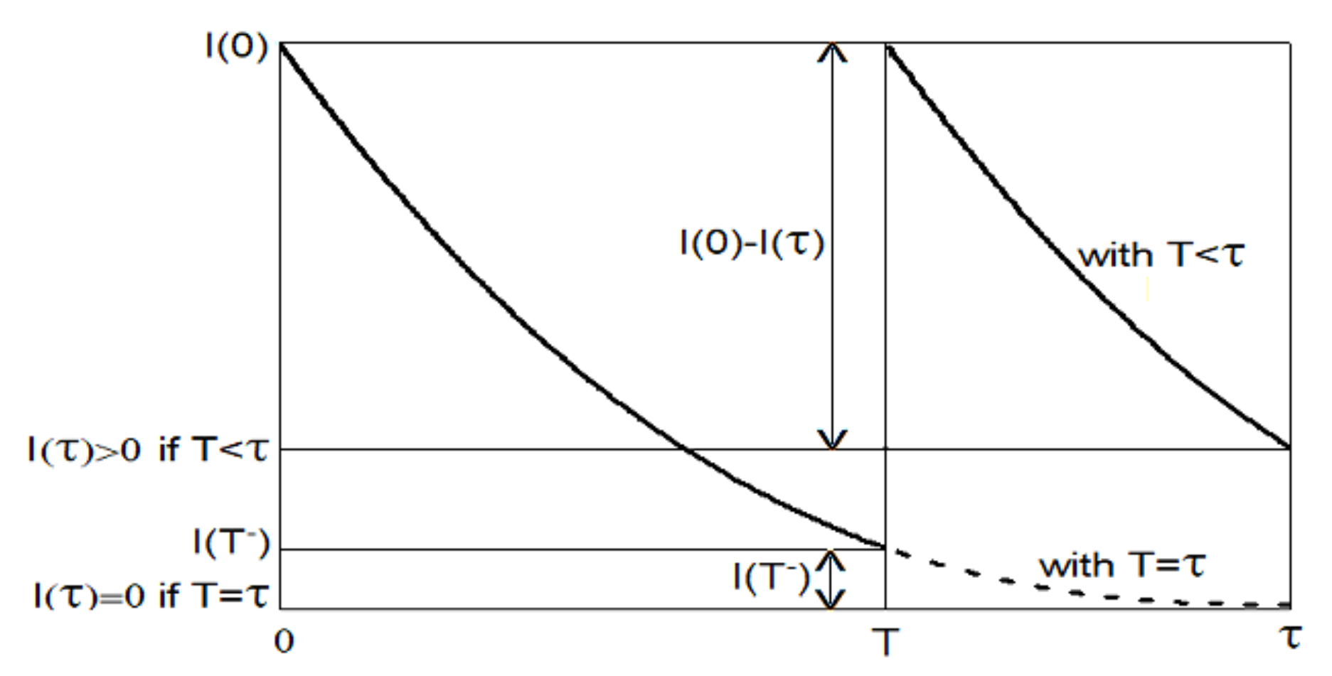
The goal of the model is the maximization of the profitability index, defined as the income/expense ratio. Taking into account that the demand rate depends on the inventory level, it could be interesting to set a new order before the stock is depleted. Indeed, it leads to an increase in the demand rate, so the income is improved, which could offset the higher ordering and holding costs. Then, the optimal length T of the inventory cycle could be strictly shorter than the time period $\tau$ that would be necessary to deplete the inventory (depletion time). As shortages are not allowed, the condition $T\le \tau$ is required in the model. Figure 1 plots the inventory level curves with $T=\tau$ and $T<\tau$ for a fixed selling price p. Note that, if $T<\tau$, the sales along the interval $\left(T,\tau \right)$ are $I\left(0\right)-I\left(\tau \right)$, while, if $T=\tau$, they are $I\left(T^{-}\right)$, with $I\left(T^{-}\right)={lim}_{t\to T^{-}}I\left(t\right)$. Then, the sales are increased by $I\left(0\right)-I\left(\tau \right)-I\left(T^{-}\right)>0$, and the income is greater. For this reason, the two decision variables $\tau$ and T are considered in the model along with the selling price p. The use of the selling price as a decision variable, in addition to the profitability index maximization, and the broad frame for the demand rate, are novelty contributions of this paper.

With these assumptions, the inventory level curve can be obtained by solving the differential equation $dI\left(t\right)/dt=-D\left(p,I\left(t\right)\right)$ with the initial condition $I\left(\tau \right)=0$. The solution is

$$I\left(t\right)={\left(\frac{(1-\beta )\lambda (\tau -t)}{{\left(\gamma +p\right)}^{\alpha }}\right)}^{1/(1-\beta )},$$

with $t\in \left[0,T\right]$.

The holding cost in a cycle $H\left(p,\tau ,T\right)$ can be evaluated as

$$H\left(p,\tau ,T\right)={\int }_0^{T}hI\left(t\right)dt=A_1\left(\frac{{\tau }^{(2-\beta )/(1-\beta )}-{\left(\tau -T\right)}^{(2-\beta )/(1-\beta )}}{{\left(\gamma +p\right)}^{\alpha /(1-\beta )}}\right),$$

(2)

where $A_1$ is an auxiliary parameter defined as:

$$A_1=\frac{h(1-\beta ){\left[(1-\beta )\lambda \right]}^{1/(1-\beta )}}{(2-\beta )}.$$

(3)

The lot size can be evaluated as a function of the decision variables as

$$q\left(p,\tau ,T\right)=I\left(0\right)-I\left(T^{-}\right)=A_2\left(\frac{{\tau }^{1/(1-\beta )}-{(\tau -T)}^{1/(1-\beta )}}{{\left(\gamma +p\right)}^{\alpha /(1-\beta )}}\right),$$

(4)

where $A_2$ is an auxiliary parameter defined as:

$$A_2={\left((1-\beta )\lambda \right)}^{1/(1-\beta )}.$$

(5)

The total cost in a cycle is the sum of the purchasing cost $cq\left(p,\tau ,T\right)$, the ordering cost K, and the holding cost $H\left(p,\tau ,T\right)$. Then, the total cost per unit time leads to

$$C\left(p,\tau ,T\right)=\frac{cq\left(p,\tau ,T\right)+K+H\left(p,\tau ,T\right)}{T}.$$

(6)

The income obtained in each inventory cycle is $pq\left(p,\tau ,T\right)$. Then, the profitability index for the system is given by:

$$W\left(p,\tau ,T\right)=\frac{pq\left(p,\tau ,T\right)}{cq\left(p,\tau ,T\right)+K+H(p,\tau ,T)}=\frac{p}{c+w\left(p,\tau ,T\right)},$$

(7)

where

$$w\left(p,\tau ,T\right)=\frac{K+H(p,\tau ,T)}{q\left(p,\tau ,T\right)}=\frac{K{\left(\gamma +p\right)}^{\alpha /(1-\beta )}+A_1\left[{\tau }^{(2-\beta )/(1-\beta )}-{\left(\tau -T\right)}^{(2-\beta )/(1-\beta )}\right]}{A_2\left[{\tau }^{1/(1-\beta )}-{(\tau -T)}^{1/(1-\beta )}\right]}.$$

(8)

The profit per unit time is given by:

$$G\left(p,\tau ,T\right)=\frac{(p-c)q\left(p,\tau ,T\right)-K-H\left(p,\tau ,T\right)}{T},$$

(9)

and it can be evaluated as

$$G\left(p,\tau ,T\right)=\left(W\left(p,\tau ,T\right)-1\right)C\left(p,\tau ,T\right).$$

(10)

Therefore, the ratio between the profit and the total cost leads to $W\left(p,\tau ,T\right)-1$. In this way, if the profitability index is, for example, $1.45$, then the system provides $1.45$ currency units per each unit spent, and the profitability of the inventory is $45\%$.

Note that $w\left(p,\tau ,T\right)>0$, and it can be seen as the average inventory cost per item (excluding the purchasing cost). Moreover, it ensures that $0<W\left(p,\tau ,T\right)<p/c$. Then, if $p\le c$, it is clear that $W\left(p,\tau ,T\right)<1$ for all the values of the decision variables, and the inventory system never yields a profit because the income is always less than the total cost. So, we suppose that $p>c$ to maximize the profitability index. Thus, the maximization problem is

$$\underset{\left(p,\tau ,T\right)\in \Omega }{max}W\left(p,\tau ,T\right),$$

(11)

where $\Omega =\left\{\left(p,\tau ,T\right)\in {\mathbb{R}}^3∕p>c,T>0,\tau \ge T\right\}$ is the feasible region.

3. The Solution of the Model

To solve the problem (11), we first consider a fixed selling price p, and then, the optimal values $\left({\tau }_p^{*},T_p^{*}\right)$ which maximize the function $W_p\left(\tau ,T\right)=W\left(p,\tau ,T\right)$ are determined. From (7), it is clear that maximizing the function $W_p(\tau ,T)$ is equivalent to minimizing the function $w_p(\tau ,T)=w\left(p,\tau ,T\right)$ given by (8). Moreover, the inequalities $0\le \tau -T<\tau$, ${\tau }^{(2-\beta )/(1-\beta )}-{\left(\tau -T\right)}^{(2-\beta )/(1-\beta )}>\tau \left[{\tau }^{1/(1-\beta )}-{\left(\tau -T\right)}^{1/(1-\beta )}\right]$, and ${\tau }^{1/(1-\beta )}-{(\tau -T)}^{1/(1-\beta )}\le {\tau }^{1/(1-\beta )}$ are true. Hence, the function $w_p(\tau ,T)$ satisfies

$$w_p(\tau ,T)>\frac{K{\left(\gamma +p\right)}^{\alpha /(1-\beta )}}{A_2{\tau }^{1/(1-\beta )}}+\frac{A_1\tau }{A_2}=w_p(\tau ,\tau ).$$

Then, for each given value p, the minimum of the function $w_p(\tau ,T)$ is obtained when $T=\tau$. Thus, the optimal length of the inventory cycle $T_p^{*}$ is equal to the optimal depletion time ${\tau }_p^{*}$. Moreover, taking into account that $A_1/A_2=h(1-\beta )/(2-\beta )$, the optimal depletion time ${\tau }_p^{*}$ can be obtained by minimizing the function $f\left(\tau \right)$ given by

$$f\left(\tau \right)=w_p(\tau ,\tau )=\frac{K{\left(\gamma +p\right)}^{\alpha /(1-\beta )}}{A_2{\tau }^{1/(1-\beta )}}+\frac{(1-\beta )h\tau }{2-\beta }.$$

The following lemma gives the solution to this problem.

Lemma 1.

Consider the function $f\left(x\right)=\frac{K{\left(\gamma +p\right)}^{\alpha /(1-\beta )}}{A_2{x}^{1/(1-\beta )}}+\frac{(1-\beta )hx}{2-\beta }$, with $x>0$ and $A_2$ given by (5). The minimum value of $f\left(x\right)$ is obtained at the point

$$x^{*}={\left({\displaystyle \frac{(2-\beta )K{\left(\gamma +p\right)}^{\alpha /(1-\beta )}}{{(1-\beta )}^2{A}_{2}h}}\right)}^{(1-\beta )/(2-\beta )},$$

with

$$f\left(x^{*}\right)=(1-\beta )h{x}^{*}=A_3{\left(\gamma +p\right)}^{\alpha /\left(2-\beta \right)},$$

where $A_3$ is an auxiliary parameter defined as:

$$A_3={\left({\displaystyle \frac{(2-\beta )K}{1-\beta }}\right)}^{\left(1-\beta \right)/\left(2-\beta \right)}{\left(\frac{h}{\lambda }\right)}^{1/\left(2-\beta \right)}.$$

(12)

Proof. 

Please see the proof in Appendix A.    □

From the previous lemma, for each given value p, the optimal cycle time $T_p^{*}$, which is equal to the optimal depletion time ${\tau }_p^{*}$, is given by

$$T_p^{*}={\tau }_p^{*}={\left({\displaystyle \frac{(2-\beta )K{\left(\gamma +p\right)}^{\alpha /(1-\beta )}}{{(1-\beta )}^2{A}_{2}h}}\right)}^{(1-\beta )/(2-\beta )},$$

(13)

where $A_2$ is given by (5), and the maximum profitability index given by (7) is:

$$W^{*}\left(p\right)=W(p,T_p^{*},T_p^{*})=\frac{p}{c+w\left(p,T_p^{*},T_p^{*}\right)}=\frac{p}{c+A_3{\left(\gamma +p\right)}^{\alpha /\left(2-\beta \right)}},$$

(14)

where $A_3$ is given by (12).

Therefore, the issue now is to look for the selling price p which maximizes the function $W^{*}\left(p\right)$ given by (14). That is, the new problem is

$$\underset{p\in \left(c,\infty \right)}{max}{W}^{*}\left(p\right).$$

(15)

Before solving it, the following lemma establishes an interesting property of the function $W^{*}\left(p\right)$.

Lemma 2.

Consider the function $W^{*}\left(p\right)$ given by (14) and the auxiliary parameter $A_3$ given by (12). Suppose that the condition

$$c+\gamma \ge {\left(\frac{2-\beta }{\alpha A_3}\right)}^{\left(2-\beta \right)/\left(\alpha -2+\beta \right)}$$

(16)

is accepted. Then, the function $W^{*}\left(p\right)$ satisfies $W^{*}\left(p\right)<1$ for all $p\in \left(c,\infty \right)$.

Proof. 

Please see the proof in Appendix A.    □

The previous lemma ensures that, if the condition (16) is satisfied, then $W\left(p,\tau ,T\right)<1$ for any values $\left(p,\tau ,T\right)\in \Omega$, and the inventory system never yields a profit because the income is always less than the total cost. So, from now on, we suppose that the parameters of the inventory system satisfy the condition

$$c+\gamma <{\left(\frac{2-\beta }{\alpha A_3}\right)}^{\left(2-\beta \right)/\left(\alpha -2+\beta \right)}.$$

(17)

This inequality is a necessary condition (but not sufficient) for the model to be profitable and to make earnings.

The derivative of the function $W^{*}\left(p\right)$ is given by

$${\left(W^{*}\right)}^{\prime }\left(p\right)=\frac{A_3\psi \left(p\right)}{{\left(c+A_3{\left(\gamma +p\right)}^{\alpha /\left(2-\beta \right)}\right)}^2},$$

with

$$\psi \left(p\right)={\left(\gamma +p\right)}^{\alpha /\left(2-\beta \right)}-\left(\frac{\alpha }{2-\beta }\right)p{\left(\gamma +p\right)}^{-1+\alpha /\left(2-\beta \right)}+\frac{c}{A_3}.$$

(18)

Then, the stationary points of the function $W^{*}\left(p\right)$ can be obtained by solving the equation $\psi \left(p\right)=0$. Taking into account that

$${\psi }^{\prime }\left(p\right)=-\left(\frac{\alpha \left(\alpha -2+\beta \right)}{{\left(2-\beta \right)}^2}\right)p{\left(\gamma +p\right)}^{-2+\alpha /\left(2-\beta \right)}<0,$$

(19)

the next theorem proves that the equation $\psi \left(p\right)=0$ has a unique solution $p^{*}\in \left(c,\infty \right)$, which can be obtained as the limit of a succession.

Theorem 1.

(Optimal selling price) Consider the functions $\psi \left(p\right)$ and ${\psi }^{\prime }\left(p\right)$ given by (18) and (19), respectively, with $p\in \left(c,\infty \right)$, and the auxiliary parameter $A_3$ given by (12). Suppose that the condition (17) is satisfied. Then, the following assertions are true:

(i)

The equation $\psi \left(p\right)=0$ has one, and only one, solution $p^{*}$ within the interval $\left(c,\infty \right)$, which satisfies $\psi \left(p\right)>0$ if $p\in \left(c,p^{*}\right)$, and $\psi \left(p\right)<0$ if $p\in \left(p^{*},\infty \right)$.

(ii)

This unique root $p^{*}$ of $\psi \left(p\right)$ satisfies $max\left(c,p_L\right)<p^{*}<p_U$, where

$$p_L={\left(\frac{\left(2-\beta \right)c}{\left(\alpha -2+\beta \right)A_3}\right)}^{\left(2-\beta \right)/\alpha }-\gamma ,$$

$$p_U=\left(\frac{2-\beta }{\alpha -2+\beta }\right)\left(\frac{c{\left(\gamma +c\right)}^{1-\alpha /\left(2-\beta \right)}}{A_3}+\gamma \right).$$

(iii)

The sequence ${\left\{y_n\right\}}_{n=1}^{\infty }$ defined by

$$y_n=y_{n-1}-\frac{\psi \left(y_{n-1}\right)}{{\psi }^{\prime }\left(y_{n-1}\right)},$$

with $y_0=p_U$, satisfies $p^{*}={lim}_{n\to \infty }{y}_n$.

Proof. 

Please see the proof in Appendix A.    □

The previous theorem ensures that the selling price $p^{*}$ is the unique stationary point of the function $W^{*}\left(p\right)$, and, moreover, it is the solution of the problem (15), because ${\left(W^{*}\right)}^{\prime }\left(p\right)>0$ if $p\in \left(c,p^{*}\right)$, and ${\left(W^{*}\right)}^{\prime }\left(p\right)<0$ if $p\in \left(p^{*},\infty \right)$. From this result, the next theorem gives the optimal policy for the inventory system, which can be obtained from the solution of the problem (11).

Theorem 2.

(Optimal policy) Suppose that the parameters of the inventory system satisfy the condition (17). Consider the optimal selling price $p^{*}$ given by Theorem 1 and the functions $W\left(p,\tau ,T\right)$ and $H(p,\tau ,T)$ given by (7) and (2), respectively. Then, the following assertions are true:

(i)

The maximum profitability index $W^{*}$ is

$$W^{*}={\left({\displaystyle \frac{(2-\beta ){\left(1-\beta \right)}^{1-\beta }\lambda }{{\alpha }^{2-\beta }h{K}^{1-\beta }{\left(\gamma +p^{*}\right)}^{\alpha -2+\beta }}}\right)}^{1/(2-\beta )}.$$

(20)

(ii)

The optimal cycle time $T^{*}$, which matches the optimal depletion time ${\tau }^{*}$, is

$$T^{*}={\tau }^{*}={\left({\displaystyle \frac{{(2-\beta )}^{1-\beta }{K}^{1-\beta }{\left(\gamma +p^{*}\right)}^{\alpha }}{{\left(1-\beta \right)}^{3-2\beta }{h}^{1-\beta }\lambda }}\right)}^{1/(2-\beta )}.$$

(21)

(iii)

The optimal lot size $q^{*}$ is

$$q^{*}={\left({\displaystyle \frac{(2-\beta )K\lambda }{\left(1-\beta \right)h{\left(\gamma +p^{*}\right)}^{\alpha }}}\right)}^{1/(2-\beta )}.$$

(22)

(iv)

The optimal policy of the inventory system satisfies the equality

$$K=\left(1-\beta \right)H\left(p^{*},T^{*},T^{*}\right),$$

where K is the ordering cost, and $H(p^{*},T^{*},T^{*})$ is the optimal holding cost in an inventory cycle.

Proof. 

Please see the proof in Appendix A.    □

The next algorithm summarizes the procedure to obtain the optimal solution of the inventory model using the previous theorems.

Remark 1.

Note that, from assertion (i) of Theorem 1, if $\psi (p_k-TOL)>0$, then $p_k-TOL<p^{*}$. Moreover, from the proof of assertion (iii) in that theorem, $p^{*}<p_k$. As a consequence, $0<p_k-p^{*}<TOL$, and this condition is a suitable stopping rule for the Algorithm 1. In addition, as can be seen in the proof of Theorem 1 given in Appendix A, the Algorithm 1 is based on the Newton’s method for solving equations. Even more, in the proof of Theorem 1, it is also proved that $\psi \left(p_0\right)=\psi \left(p_U\right)<0$ and ${\psi }^{″}\left(p_0\right)<0$. Then, the Newton’s method converges in a quadratic and monotonous way to the only root of the function $\psi \left(p\right)$ (see, for example, Householder [29], Theorem 4.2.4).

Algorithm 1:Obtaining the optimal policy and the maximum profitability index.

(i) Calculate the auxiliary parameter$A_3={\left(\frac{(2-\beta )K}{1-\beta }\right)}^{\left(1-\beta \right)/\left(2-\beta \right)}{\left(\frac{h}{\lambda }\right)}^{1/(2-\beta )}$. (ii) If $c+\gamma \ge {\left(\frac{2-\beta }{\alpha A_3}\right)}^{\left(2-\beta \right)/\left(\alpha -2+\beta \right)}$, then stop; the inventory system is not profitable. Otherwise, go to Step (iii). (iii) Consider the function $\psi \left(p\right)={\left(\gamma +p\right)}^{\alpha /\left(2-\beta \right)}-\left(\frac{\alpha }{2-\beta }\right)p{\left(\gamma +p\right)}^{-1+\alpha /\left(2-\beta \right)}+\frac{c}{A_3}$ and its derivative ${\psi }^{\prime }\left(p\right)=-\left(\frac{\alpha \left(\alpha -2+\beta \right)}{{\left(2-\beta \right)}^2}\right)p{\left(\gamma +p\right)}^{-2+\alpha /\left(2-\beta \right)}$. Select a tolerance parameter $TOL>0$ for determining the selling price. (iv) Set $p_0=\left(\frac{2-\beta }{\alpha -2+\beta }\right)\left(\frac{c{\left(\gamma +c\right)}^{1-\alpha /\left(2-\beta \right)}}{A_3}+\gamma \right)$. (v) Calculate $p_i=p_{i-1}-{\displaystyle \frac{\psi \left(p_{i-1}\right)}{{\psi }^{\prime }\left(p_{i-1}\right)}}$ for $i=1,2,3...$ until the first index k that satisfies $\psi (p_k-TOL)>0$ is reached. (vi) Take the value $p^{*}=p_k$ as the optimal selling price. (vii) Evaluate the optimal cycle time as $T^{*}={\left(\frac{{(2-\beta )}^{1-\beta }{K}^{1-\beta }{\left(\gamma +p^{*}\right)}^{\alpha }}{{\left(1-\beta \right)}^{3-2\beta }{h}^{1-\beta }\lambda }\right)}^{1/(2-\beta )}$. (viii) Obtain the maximum profitability index as $W^{*}={\left(\frac{(2-\beta ){\left(1-\beta \right)}^{1-\beta }\lambda }{{\alpha }^{2-\beta }h{K}^{1-\beta }{\left(\gamma +p^{*}\right)}^{\alpha -2+\beta }}\right)}^{1/(2-\beta )}$. (ix) Determine the optimal lot size as $q^{*}={\left(\frac{(2-\beta )K\lambda }{\left(1-\beta \right)h{\left(\gamma +p^{*}\right)}^{\alpha }}\right)}^{1/(2-\beta )}$.

Besides, if the demand rate does not depend on the stock level, that is $\beta =0$, for any values of the parameters $\alpha$ and $\gamma$, the ordering cost is equal to the holding cost, just as Harris’ rule establishes for the basic EOQ model. Otherwise, if $0<\beta <1$, then $K<H\left(p^{*},T^{*},T^{*}\right)$, i.e., the ordering cost is less than the holding cost. Moreover, the inventory cost in each cycle is $K+H\left(p^{*},T^{*},T^{*}\right)=\left(2-\beta \right)K/(1-\beta )$, and the average inventory cost per item, given by (8), can be evaluated for the optimal solution as

$$w^{*}=w\left(p^{*},T^{*},T^{*}\right)=\frac{\left(2-\beta \right)K}{(1-\beta )q^{*}}.$$

(23)

Then, from (7), the maximum profitability index is also given by

$$W^{*}=\frac{p^{*}}{c+\frac{\left(2-\beta \right)K}{(1-\beta )q^{*}}},$$

(24)

which is the ratio between the income per item and the average total cost per item.

In addition, using the expressions (20) and (22), the ratio between the optimal lot size and the maximum profitability index is

$$\frac{q^{*}}{W^{*}}=\frac{\alpha K}{\left(1-\beta \right)\left(\gamma +p^{*}\right)}.$$

Then, the total cost per unit time for the optimal solution, given by (6), could also be evaluated as

$$\begin{array}{ccc}\hfill C\left(p^{*},T^{*},T^{*}\right)& =& \frac{p^{*}{q}^{*}}{T^{*}{W}^{*}}=\left(\frac{\alpha K{p}^{*}}{\left(1-\beta \right){\left(\gamma +p^{*}\right)}^{1+\alpha /\left(2-\beta \right)}}\right){\left(\frac{{\left(1-\beta \right)}^{3-2\beta }{h}^{1-\beta }\lambda }{{(2-\beta )}^{1-\beta }{K}^{1-\beta }}\right)}^{1/(2-\beta )}\hfill \\ & =& \left(\frac{\alpha {\left(K\lambda \right)}^{1/\left(2-\beta \right)}{p}^{*}}{{\left(\gamma +p^{*}\right)}^{1+\alpha /\left(2-\beta \right)}}\right){\left({\displaystyle \frac{\left(1-\beta \right)h}{2-\beta }}\right)}^{(1-\beta )/(2-\beta )}.\hfill \end{array}$$

(25)

Similarly, the profit per unit time for this optimal solution, i.e., $G\left(p^{*},T^{*},T^{*}\right)$, could be evaluated as

$$G\left(p^{*},T^{*},T^{*}\right)=(W^{*}-1)C\left(p^{*},T^{*},T^{*}\right).$$

The inventory system would be profitable if, and only if, the income is strictly greater than the total cost, i.e., if and only if $W^{*}>1$. Taking into account that $\psi \left(p^{*}\right)=0$, from (18), the optimal selling price $p^{*}$ satisfies $c+A_3{\left(\gamma +p^{*}\right)}^{\alpha /\left(2-\beta \right)}=\left(\frac{\alpha A_3}{2-\beta }\right)p^{*}{\left(\gamma +p^{*}\right)}^{-1+\alpha /\left(2-\beta \right)}$. Then, the expression (14) can be used to obtain a profitability condition for the inventory as follows:

$$W^{*}>1\iff \frac{2-\beta }{\alpha A_3{\left(\gamma +p^{*}\right)}^{-1+\alpha /\left(2-\beta \right)}}>1\iff p^{*}<-\gamma +{\left(\frac{2-\beta }{\alpha A_3}\right)}^{\left(2-\beta \right)/\left(\alpha -2+\beta \right)}.$$

(26)

From (26), the next lemma provides a profitability condition which only depends on the initial parameters of the model and allows the profitability threshold to be obtained for each parameter, keeping all the others fixed.

Lemma 3.

Suppose that the parameters of the inventory model satisfy the condition (17). Then, the inventory system is profitable if, and only if, the following inequality:

$${\displaystyle \frac{h{K}^{1-\beta }{\left(c+\gamma \right)}^{\alpha -2+\beta }}{\lambda }}<\Delta$$

(27)

is satisfied, where

$$\Delta =\frac{\left(2-\beta \right){\left(1-\beta \right)}^{1-\beta }{\left(\alpha -2+\beta \right)}^{\alpha -2+\beta }}{{\alpha }^{\alpha }}$$

(28)

is an auxiliary parameter which only depends on the two elasticity parameters of the model.

Proof. 

Please see the proof in Appendix A. □

Therefore, the inequality (27) provides a necessary and sufficient condition to be a profitable model and generate earnings. Moreover, from this condition, it is possible to deduce profitability thresholds for the parameters $K,h,c,\lambda ,$ and $\gamma$, keeping all the others fixed.

Table 1. Profitability thresholds for the parameters $K,h,c,\lambda ,$ and $\gamma$ of the inventory system.

Parameter:	$\mathit{K}<$	$\mathit{h}<$	$\mathit{c}<$	$\mathit{\lambda }>$	$\mathit{\gamma }<$
Threshold:	${\left({\displaystyle \frac{\lambda \Delta }{h\theta }}\right)}^{1/(1-\beta )}$	${\displaystyle \frac{\lambda \Delta }{K^{1-\beta }\theta }}$	$-\gamma +{\left({\displaystyle \frac{\lambda \Delta }{K^{1-\beta }h}}\right)}^{1/\left(\alpha -2+\beta \right)}$	${\displaystyle \frac{h{K}^{1-\beta }\theta }{\Delta }}$	$-c+{\left({\displaystyle \frac{\lambda \Delta }{K^{1-\beta }h}}\right)}^{1/\left(\alpha -2+\beta \right)}$

collects these thresholds, where the notation $\theta ={\left(c+\gamma \right)}^{\alpha -2+\beta }$ is used.

4. Sensitivity Analysis of the Optimal Policy

This section conducts a sensitivity analysis for the optimal solution, by using their partial derivatives regarding the parameters K, h, $\lambda$, c, and $\gamma$.

The sensitivity of the optimal selling price $p^{*}$ with respect to these parameters is analyzed in the next corollary.

Corollary 1.

Let $p^{*}$ be the optimal selling price given by Theorem 1. Then:

(i)

$p^{*}$ decreases as the ordering cost K, or the holding cost h per unit and per unit time, increases.

(ii)

$p^{*}$ increases as the scale parameter λ of the demand rate, or the purchasing cost c, increases.

(iii)

$p^{*}$ decreases as the non-centrality parameter γ increases if the condition $\left(2-\alpha /\left(2-\beta \right)\right)p^{*}+\gamma <0$ is satisfied. Otherwise, $p^{*}$ increases as γ increases.

Proof. 

Please see the proof in Appendix A. □

Remark 2.

The expressions for the partial derivatives of $p^{*}$ obtained in this proof lead to

$$\begin{array}{ccc}\hfill \frac{\partial p^{*}}{\partial K}& =& \frac{(1-\beta )h}{K}\frac{\partial p^{*}}{\partial h}<0,\hfill \\ \hfill \frac{\partial p^{*}}{\partial \lambda }& =& \frac{-h}{\lambda }\frac{\partial p^{*}}{\partial h}>0,\hfill \\ \hfill \frac{\partial p^{*}}{\partial c}& =& -\frac{(2-\beta )h}{c}\frac{\partial p^{*}}{\partial h}>0.\hfill \end{array}$$

Thus,

$$\frac{\partial p^{*}/\partial c}{p^{*}/c}>\left|\frac{\partial p^{*}/\partial h}{p^{*}/h}\right|=\frac{\partial p^{*}/\partial \lambda }{p^{*}/\lambda }\ge \left|\frac{\partial p^{*}/\partial K}{p^{*}/K}\right|$$

because $2-\beta >1\ge 1-\beta$. As a consequence, the relative change in the optimal selling price $p^{*}$ is greater regarding the parameter c, later with respect to the parameter h or λ (which are equal), and lower concerning the parameter K.

Next, the following corollary uses the closed expression (20) to develop a sensitivity analysis of the maximum profitability index.

Corollary 2.

Let $W^{*}$ be the maximum profitability index given by (20). Then:

(i)

$W^{*}$ decreases as any of the parameters K, h, c, or γ increases.

(ii)

$W^{*}$ increases as the scale parameter λ of the demand rate increases.

Proof. 

Please see the proof in Appendix A. □

Remark 3.

The expressions for the partial derivatives of $W^{*}$ obtained in this proof lead to

$$\begin{array}{ccc}\hfill \frac{\partial W^{*}}{\partial K}& =& \frac{(1-\beta )h}{K}\frac{\partial W^{*}}{\partial h}<0,\hfill \\ \hfill \frac{\partial W^{*}}{\partial \lambda }& =& \frac{-h}{\lambda }\frac{\partial W^{*}}{\partial h}>0;\hfill \end{array}$$

therefore,

$$\left|\frac{\partial W^{*}/\partial h}{W^{*}/h}\right|=\frac{\partial W^{*}/\partial \lambda }{W^{*}/\lambda }\ge \left|\frac{\partial W^{*}/\partial K}{W^{*}/K}\right|$$

because $1-\beta \le 1$. As a consequence, the maximum profitability index $W^{*}$ is equally sensitive regarding the parameters h and λ, and more sensitive, with respect to these parameters h or λ, than to the parameter K.

In a similar way, a sensitivity analysis of the optimal cycle time $T^{*}$ is performed in the next corollary by using the closed expression (21).

Corollary 3.

Let $T^{*}$ be optimal cycle time given by (21). Then:

(i)

$T^{*}$ decreases as the holding cost h per unit and per unit time, or the scale parameter λ of the demand rate, increases.

(ii)

$T^{*}$ increases as any of the parameters K, c, or γ increases.

Proof. 

Please see the proof in Appendix A. □

Finally, the following corollary shows the sensitivity analysis of the optimal lot size $q^{*}$, which is given by the expression (22).

Corollary 4.

Let $q^{*}$ be optimal lot size given by (22). Then:

(i)

$q^{*}$ increases as the ordering cost K, or the scale parameter λ of the demand rate, increases.

(ii)

$q^{*}$ decreases as any of the parameters h, c, or γ increases.

Proof. 

Please see the proof in Appendix A. □

In summary, the following bullet list collects the behavior of the optimal policy when one of the parameters varies, keeping all the others fixed:

• If the ordering cost K increases, then the optimal values $p^{*}$ and $W^{*}$ decrease, while the optimal values $T^{*}$ and $q^{*}$ increase.
• If the holding cost h per unit and per unit time increases, then all optimal values $p^{*}$, $W^{*}$, $T^{*}$, and $q^{*}$ decrease.
• If the scale parameter $\lambda$ of the demand rate increases, then the optimal values $p^{*}$, $W^{*}$, and $q^{*}$ increase, while the optimal value $T^{*}$ decreases.
• If the unit purchasing cost c increases, then the optimal values $p^{*}$ and $T^{*}$ increase, while the optimal values $W^{*}$ and $q^{*}$ decrease.
• If the non-centrality parameter $\gamma$ increases, then the optimal values $W^{*}$ and $q^{*}$ decrease, while $T^{*}$ increases. However, if $\gamma$ increases, then the optimal selling price $p^{*}$ can increase or decrease depending on what its value is.

5. The Case of the Isoelastic Price-Dependent Demand

A special case of the model solved in the previous section is the inventory system with stock-dependent and isoelastic price-dependent demand, which is obtained with $\gamma =0$ in the expression (1). In this case, the demand function is

$$D\left(p,I\left(t\right)\right)=\lambda p^{-\alpha }{\left(I\left(t\right)\right)}^{\beta },$$

and the inventory level curve is

$$I\left(t\right)={\left((1-\beta )\lambda p^{-\alpha }(\tau -t)\right)}^{1/(1-\beta )},$$

with $t\in \left[0,T\right]$.

The auxiliary parameters $A_1$, $A_2$, and $A_3$, given by (3), (5), and (12), respectively, do not change because they do not depend on $\gamma$.

Now, the function $\psi \left(p\right)$ given by (18) can be written as

$$\psi \left(p\right)=-\left(\frac{\alpha -2+\beta }{2-\beta }\right)p^{\alpha /\left(2-\beta \right)}+\frac{c}{A_3},$$

and the solution of the equation $\psi \left(p\right)=0$ can be obtained in a closed form as

$$p_0^{*}={\left(\frac{\left(2-\beta \right)c}{\left(\alpha -2+\beta \right)A_3}\right)}^{\left(2-\beta \right)/\alpha }.$$

Moreover, substituting $A_3$ in the above expression with its value given by (12), the optimal selling price is

$$p_0^{*}={\left(\frac{(2-\beta ){\left(1-\beta \right)}^{1-\beta }\lambda c^{2-\beta }}{{\left(\alpha -2+\beta \right)}^{2-\beta }h{K}^{1-\beta }}\right)}^{1/\alpha }.$$

(29)

The optimal cycle time $T_0^{*}$, given by the expression (21) with $\gamma =0$, leads to

$$T_0^{*}={\left(\frac{{(2-\beta )}^{1-\beta }{K}^{1-\beta }{\left(p_0^{*}\right)}^{\alpha }}{{\left(1-\beta \right)}^{3-2\beta }{h}^{1-\beta }\lambda }\right)}^{1/(2-\beta )}=\frac{(2-\beta )c}{\left(\alpha -2+\beta \right)\left(1-\beta \right)h}.$$

(30)

The maximum profitability index, given by (20) with $\gamma =0$, leads to

$$W_0^{*}={\left({\displaystyle \frac{(2-\beta ){\left(1-\beta \right)}^{1-\beta }\lambda }{{\alpha }^{2-\beta }h{K}^{1-\beta }{\left(p_0^{*}\right)}^{\alpha -2+\beta }}}\right)}^{1/(2-\beta )}={\left(\frac{(2-\beta ){\left(1-\beta \right)}^{1-\beta }{(\alpha -2+\beta )}^{\alpha -2+\beta }\lambda }{{\alpha }^{\alpha }h{K}^{1-\beta }{c}^{\alpha -2+\beta }}\right)}^{1/\alpha }.$$

(31)

Finally, the optimal lot size $q_0^{*}$ can be obtained from the expression (22), with $\gamma =0$, as

$$q_0^{*}={\left({\displaystyle \frac{(2-\beta )K\lambda }{\left(1-\beta \right)h{\left(p_0^{*}\right)}^{\alpha }}}\right)}^{1/(2-\beta )}=\frac{\left(\alpha -2+\beta \right)K}{\left(1-\beta \right)c}.$$

(32)

Then, in this case, all the values for the optimal policy of the inventory system can be obtained by a closed form. These optimal values only depend on the initial parameters of the model. Therefore, these expressions are general, and they can be applied whatever the values of the initial parameters are. Furthermore, these expressions lead to some interesting conclusions, which can be extended and used in practical applications of the model. They are listed below.

(i) First of all, from (7), $p_0^{*}/c$ would be the profitability index if there were no inventory cost. Now, in the system with an isoelastic price dependent demand, from (24) and (32), the optimal profitability index $W_0^{*}$ satisfies the equality

$$\frac{W_0^{*}}{p_0^{*}/c}=1-\frac{2-\beta }{\alpha }.$$

Thus, the ratio $\left(2-\beta \right)/\alpha$ is the relative drop in the profitability index due to the inventory cost.

(ii) Note that, in this model, neither the optimal cycle time $T_0^{*}$ nor the optimal lot size $q_0^{*}$ depend on the scale parameter $\lambda$ of the demand rate. In addition, the optimal cycle time $T_0^{*}$ does not depend on the ordering cost K, and the optimal lot size $q_0^{*}$ does not depend on the parameter h of the holding cost.

(iii) Moreover, from (29), the optimal selling price $p_0^{*}$ increases if the parameters c or $\lambda$ increase, and it decreases if the parameters K or h increase. Similarly, from (30), the optimal length of the cycle time $T_0^{*}$ decreases if the parameter h increases, and it increases if the parameter c increases. In addition, from (31), the maximum profitability index $W_0^{*}$ increases if the parameter $\lambda$ increases, and it decreases if any of the parameters K, h or c increase. Finally, from (32), the optimal lot size $q_0^{*}$ increases if the parameter K increases, and it decreases if the parameter c increases.

The relative effect of the parameter K on the maximum profitability index $W_0^{*}$, given by (31), can be evaluated as

$$\frac{\partial W_0^{*}/\partial K}{W_0^{*}/K}=K\left(\frac{\partial ln\left(W_0^{*}\right)}{\partial K}\right)=-\left(\frac{1-\beta }{\alpha }\right).$$

Similarly, for the parameters h, $\lambda$, and c, the expressions for the relative effects of these parameters on $W_0^{*}$ are

$$\frac{\partial W_0^{*}/\partial h}{W_0^{*}/h}=-\left(\frac{1}{\alpha }\right)=-\left(\frac{\partial W_0^{*}/\partial \lambda }{W_0^{*}/\lambda }\right),$$

and

$$\frac{\partial W_0^{*}/\partial c}{W_0^{*}/c}=-\left(\frac{\alpha -2+\beta }{\alpha }\right).$$

Therefore, the relation between these quantities is

$$\left|\frac{\partial W_0^{*}/\partial h}{W_0^{*}/h}\right|=\left(\frac{\partial W_0^{*}/\partial \lambda }{W_0^{*}/\lambda }\right)\ge \left|\frac{\partial W_0^{*}/\partial K}{W_0^{*}/K}\right|.$$

As a consequence, the maximum profitability index is more sensitive with respect to the parameters h or $\lambda$ than to the parameter K. The sensitivity with respect to the parameter c can be greater or lower than concerning the parameters h, $\lambda$, or K, depending on the value $\alpha -2+\beta$.

In a similar way, the relative effects of the parameters K, h, and c on the optimal selling price $p_0^{*}$ are given by the expressions

$$\frac{\partial p_0^{*}/\partial K}{p_0^{*}/K}=K\left(\frac{\partial ln\left(p_0^{*}\right)}{\partial K}\right)=-\left(\frac{1-\beta }{\alpha }\right),$$

$$\frac{\partial p_0^{*}/\partial h}{p_0^{*}/h}=-\left(\frac{1}{\alpha }\right)=-\left(\frac{\partial p_0^{*}/\partial \lambda }{p_0^{*}/\lambda }\right),$$

$$\frac{\partial p_0^{*}/\partial c}{p_0^{*}/c}=\frac{2-\beta }{\alpha }.$$

Therefore, the relation between these quantities is

$$\frac{\partial p_0^{*}/\partial c}{p_0^{*}/c}>\left|\frac{\partial p_0^{*}/\partial h}{p_0^{*}/h}\right|=\frac{\partial p_0^{*}/\partial \lambda }{p_0^{*}/\lambda }\ge \left|\frac{\partial p_0^{*}/\partial K}{p_0^{*}/K}\right|.$$

As a consequence, the optimal selling price $p_0^{*}$, given by (29), is first more sensitive regarding the parameter c, then with respect to the parameter h or $\lambda$, and less sensitive concerning the parameter K. In addition, the relative effects of the parameters K, h, and $\lambda$ on the maximum profitability index $W_0^{*}$ and on the optimal selling price $p_0^{*}$ are equal.

As expected, all these results agree with the ones obtained in Section 4.

With respect to the optimal length of the inventory cycle $T_0^{*}$, given by (30), the results are

$$\left|\frac{\partial T_0^{*}/\partial h}{T_0^{*}/h}\right|=1=\frac{\partial T_0^{*}/\partial c}{T_0^{*}/c},$$

and $T_0^{*}$ is equally sensitive regarding the parameters h and c, but with the opposite sign. As stated before, it does not depend on the parameters K or $\lambda$.

Finally, for the optimal lot size $q_0^{*}$, given by (32), the results are

$$\frac{\partial q_0^{*}/\partial K}{q_0^{*}/K}=1=\left|\frac{\partial q_0^{*}/\partial c}{q_0^{*}/c}\right|.$$

Therefore, the optimal lot size $q_0^{*}$ is equally sensitive concerning the parameters K and c, but with the opposite sign. As stated before, it does not depend on the parameters h or $\lambda$.

Note that, all these statements are based on the partial derivatives of the optimal solution with respect to the initial parameters. As a result, they can be completely generalized for all the practical applications of the model.

The total cost of the system per unit time can be evaluated by placing $\gamma =0$ in the expression (25), taking into account the value $p_0^{*}$ given by (29). Then,

$$C\left(p_0^{*},T_0^{*},T_0^{*}\right)={\left({\displaystyle \frac{\left(1-\beta \right)h}{2-\beta }}\right)}^{(1-\beta )/(2-\beta )}\left(\frac{\alpha {\left(K\lambda \right)}^{1/\left(2-\beta \right)}}{{\left(p_0^{*}\right)}^{\alpha /\left(2-\beta \right)}}\right)=\frac{\left(\alpha -2+\beta \right)\alpha Kh}{(2-\beta )c}.$$

Taking into account the Equation (10), the profit per unit time for the optimal solution can be evaluated as

$$G\left(p_0^{*},T_0^{*},T_0^{*}\right)=(W_0^{*}-1)C\left(p_0^{*},T_0^{*},T_0^{*}\right).$$

This section, Section 5, has introduced a special case of the model previously solved in Section 2 and Section 3. This special case is the inventory system with stock-dependent and isoelastic price-dependent demand, and it is obtained by placing $\gamma =0$ on the expression (1). Moreover, if the value $\beta =0$ is also set in the expression (1), we are then dealing with an inventory model where the demand depends on the price, but not on the inventory level. That is, the conditions $\gamma =0$ and $\beta =0$, placed together in the expression (1), lead us to an inventory model with price-dependent demand, and such a demand does not depend on the inventory level. In this case, the demand rate function is $D\left(p\right)=\lambda p^{-\alpha }$; and the inventory level curve is $I\left(t\right)=\lambda p^{-\alpha }\left(\tau -t\right)$, with $t\in \left[0,T\right]$. Then, setting $\beta =0$ in the expressions (29)–(32), the optimal inventory policy is given by

Table 2. Optimal policy in the inventory model with an isoelastic price-dependent demand, when such a demand does not depend on the inventory level.

Selling Price	Cycle Time	Profitability Index	Lot Size
$p_1^{*}={\left({\displaystyle \frac{2\lambda c^2}{{\left(\alpha -2\right)}^{2}hK}}\right)}^{1/\alpha }$	$T_1^{*}={\displaystyle \frac{2c}{\left(\alpha -2\right)h}}$	$W_1^{*}={\left({\displaystyle \frac{2{\left(\alpha -2\right)}^{\alpha -2}\lambda }{{\alpha }^{\alpha }Kh{c}^{\alpha -2}}}\right)}^{1/\alpha }$	$q_1^{*}={\displaystyle \frac{\left(\alpha -2\right)K}{c}}$

.

6. Computational Results

In this section, the proposed model and the solution methodology are illustrated with a numerical example. Let us suppose that the purchasing cost for the item is $c=20$ currency units, the ordering cost for a new replenishment is $K=1000$ currency units, and the holding cost per unit and per unit time (a week) for the inventory system is $h=5$ currency units. Consider that the elasticity parameters for the demand rate are $\alpha =4$ and $\beta =0.2$, the non-centrality parameter is $\gamma =3$, and the potential consumers are $\Lambda =300$ per week. Then, the scale parameter of the demand function is $\lambda =300\times {23}^4=\mathrm{83,952,300}$.

Placing the values of these initial parameters on the expressions (12) and (28), the auxiliary parameters $A_3$ and $\Delta$ are calculated. Their values are $A_3=0.0030$ and $\Delta =0.0333$. First, to be sure that this inventory system could be profitable, it is verified that these numerical data satisfy the inequality (17), which is a necessary condition for the inventory system to be profitable. As these numerical data satisfy this required condition, the process goes forward to find the optimal policy of this inventory system. Therefore, Algorithm 1 is applied and the optimal policy is found. The obtained results are $p^{*}=47.62$ for the optimal selling price, $T^{*}=4.58$ weeks for the optimal cycle time, $q^{*}=122.7$ for the optimal lot size, and $W^{*}=1.2422$ for the maximum profitability index. Then, the profitability of the inventory system is $24.22\%$.

The correctness of these results is checked in the following way. Applying the expression (2), it is found that the holding cost in an inventory cycle is $H\left(p^{*},T^{*},T^{*}\right)=1250$. Applying the expression (6), it is calculated that the total cost per unit time is $C\left(p^{*},T^{*},T^{*}\right)=1025.91$. As the income per unit time is $p^{*}{q}^{*}/T^{*}=1274.34$, the profitability index for the inventory system, obtained from (25), is $W^{*}=\frac{p^{*}{q}^{*}}{T^{*}C\left(p^{*},T^{*},T^{*}\right)}=\frac{1274.34}{1025.91}=1.2422$. This value coincides with the maximum profitability index given by the algorithm. In addition, the average inventory cost per item is $w^{*}=(K+H\left(p^{*},T^{*},T^{*}\right))/q^{*}=\left(1000+1250\right)/122.7=18.34$. This value is the same value provided by the expression (23) because it is $w^{*}=(2-\beta )K/\left((1-\beta )q^{*}\right)=18.34$. Similarly, the ordering cost $K=1000$ coincides with the value $\left(1-\beta \right)H\left(p^{*},T^{*},T^{*}\right)=0.8\times 1250=1000$, as stated in assertion (iv) of Theorem 2.

It is also interesting to know the optimal solution for the problem of maximizing the profit per unit time given by the objective function (9). This is the objective frequently used in the literature on the subject. So, for this numerical example, the optimal policy of this problem has been determined by using a numerical algorithm. The obtained optimal solution is $p_G=31.89$, $T_G=2.20$, ${\tau }_G=2.21$, and $q_G=316.0$, with an optimal profit per unit time of $G^{*}=548.65$. Note that, in this case, the optimal cycle time does not match the optimal depletion time, because $T_G<{\tau }_G$. The profitability index for this solution is $W\left(p_G,{\tau }_G,T_G\right)=1.1359$, which is less than the optimal profitability index obtained, i.e., $W^{*}=1.2422$. Indeed, the profit per unit time for the maximum profitability index solution is $G\left(p^{*},{\tau }^{*},T^{*}\right)=248.43$, which is less than the optimal profit per unit, i.e., $G^{*}=548.65$. Then, both solutions are different in the selling price, the cycle time, and the lot size. In addition, the differences in the profitability index and in the profit per unit time are remarkable.

Next, the profitability thresholds for the parameters $K,h,c,\lambda ,$ and $\gamma$, keeping all the others fixed, have been calculated taking into account the expressions collected in Table 1. The obtained values are shown in

Table 3. Profitability thresholds for the initial parameters of the analyzed inventory system.

	K	h	c	λ	γ
Actual value	$1000$	$5$	$20$	$\mathrm{83,952,300}$	$3$
Profitability threshold	$K<2754.99$	$h<11.25$	$c<30.25$	$\lambda >\mathrm{37,319,586}$	$\gamma <13.25$

.

Then, the inventory system is profitable if the ordering cost K is at most $2754.99$, the holding cost per unit and per unit time h is at most $11.25$, and the purchasing cost c is at most $30.25$. As the profitability threshold for the parameter $\lambda$ is 37,319,586, the minimum number of potential customers is $\Lambda =\lambda {\left(\gamma +c\right)}^{-\alpha }=134$ customers per week. Finally, the maximum value for the parameter $\gamma$ is $13.25$.

To analyze how the optimal policy varies with the parameters of the model, they have been changed one by one, keeping the others fixed, and the optimal values $p^{*}$, $T^{*}$, $W^{*}$ and $q^{*}$ have been evaluated again. Specifically, for each parameter, we have chosen size drops of $-15\%$, $-10\%$, and $-5\%$, and increments of $5\%$, $10\%$, and $15\%$. The obtained results are shown in

Table 4. Optimal policy of the model for different values of the initial parameters.

x		$\Delta x=-15\%$	$\Delta x=-10\%$	$\Delta x=-5\%$	$\Delta x=5\%$	$\Delta x=10\%$	$\Delta x=15\%$
	$p^{*}$	$49.21$	$48.65$	$48.12$	$47.16$	$46.72$	$46.30$
$K=1000$	$T^{*}$	$4.57$	$4.57$	$4.58$	$4.59$	$4.60$	$4.60$
	$W^{*}$	$1.2858$	$1.2703$	$1.2558$	$1.2293$	$1.2172$	$1.2058$
	$q^{*}$	$104.7$	$110.7$	$116.7$	$128.7$	$134.7$	$140.6$
	$p^{*}$	$49.62$	$48.91$	$48.24$	$47.04$	$46.49$	$45.98$
$h=5$	$T^{*}$	$5.37$	$5.08$	$4.82$	$4.37$	$4.18$	$4.00$
	$W^{*}$	$1.2969$	$1.2774$	$1.2592$	$1.2261$	$1.2111$	$1.1968$
	$q^{*}$	$123.2$	$123.1$	$122.9$	$122.5$	$122.3$	$122.2$
	$p^{*}$	$44.24$	$45.40$	$46.53$	$48.69$	$49.73$	$50.74$
$c=20$	$T^{*}$	$3.93$	$4.15$	$4.37$	$4.80$	$5.02$	$5.24$
	$W^{*}$	$1.3518$	$1.3122$	$1.2758$	$1.2109$	$1.1818$	$1.1547$
	$q^{*}$	$143.1$	$135.6$	$128.8$	$117.1$	$112.1$	$107.4$
	$p^{*}$	$45.71$	$46.38$	$47.01$	$48.21$	$48.78$	$49.33$
$\lambda =$	$T^{*}$	$4.61$	$4.60$	$4.59$	$4.58$	$4.57$	$4.57$
83,952,300	$W^{*}$	$1.1896$	$1.2078$	$1.2253$	$1.2584$	$1.2741$	$1.2891$
	$q^{*}$	$122.1$	$122.3$	$122.5$	$122.9$	$123.0$	$123.2$
	$p^{*}$	$113.17$	$81.82$	$61.46$	$37.87$	$30.76$	$25.45$
$\alpha =4$	$T^{*}$	$5.95$	$5.38$	$4.94$	$4.30$	$4.07$	$3.89$
	$W^{*}$	$2.5835$	$1.9704$	$1.5462$	$1.0176$	$0.8475$	$0.7158$
	$q^{*}$	$94.5$	$104.5$	$113.9$	$130.7$	$138.1$	$144.7$
	$p^{*}$	$46.97$	$47.18$	$47.40$	$47.85$	$48.09$	$48.33$
$\beta =0.2$	$T^{*}$	$4.60$	$4.60$	$4.59$	$4.58$	$4.58$	$4.57$
	$W^{*}$	$1.2053$	$1.2174$	$1.2297$	$1.2548$	$1.2677$	$1.2808$
	$q^{*}$	$115.4$	$117.8$	$120.2$	$125.2$	$127.9$	$130.6$
	$p^{*}$	$47.68$	$47.66$	$47.64$	$47.60$	$47.59$	$47.57$
$\gamma =3$	$T^{*}$	$4.51$	$4.53$	$4.56$	$4.61$	$4.64$	$4.66$
	$W^{*}$	$1.2539$	$1.2500$	$1.2461$	$1.2382$	$1.2344$	$1.2305$
	$q^{*}$	$124.8$	$124.1$	$123.4$	$122.0$	$121.3$	$120.6$

.

From the results obtained in this sensitivity analysis, the following managerial insights are deduced. The optimal selling price $p^{*}$ and the maximum profitability index $W^{*}$ increase if the parameters $\lambda$ or $\beta$ increase, and they decrease when the other parameters increase. The optimal cycle time $T^{*}$ increases if the parameters c or $\gamma$ increase, and it does not increase when the other parameters increase. Regarding the optimal lot size $q^{*}$, it increases if any of the parameters K, $\lambda$, $\alpha$, or $\beta$ increase, and it decreases when the rest of the parameters increase.

In addition, for all the optimal values, the changes regarding the price elasticity parameter $\alpha$ are much larger than for the rest of the parameters. For example, note that the profitability index increases to $2.58$ if the parameter $\alpha$ decreases by $15\%$, and it falls to $0.72$ if the parameter $\alpha$ increases by $15\%$. However, with respect to the unit purchasing cost c, the profitability index moves between $1.35$ and $1.15$, and the changes are even smaller regarding the other parameters. The unit purchasing cost c seems to be the second most influential parameter in the optimal policy.

The ordering cost K is more influential in the optimal lot size $q^{*}$, which moves between $104.7$ and $140.6$, than in the optimal cycle time $T^{*}$, which moves between $4.57$ and $4.60$. On the other hand, the holding cost h per unit and per unit time is more influential in the optimal cycle time $T^{*}$, which moves between $4.00$ and $5.37$, than in the optimal lot size, which moves between $122.2$ and $123.2$. Finally, note that the parameter $\gamma$ seems to be less influential in the optimal policy because all the optimal values change little when it moves between $-15\%$ and $15\%$.

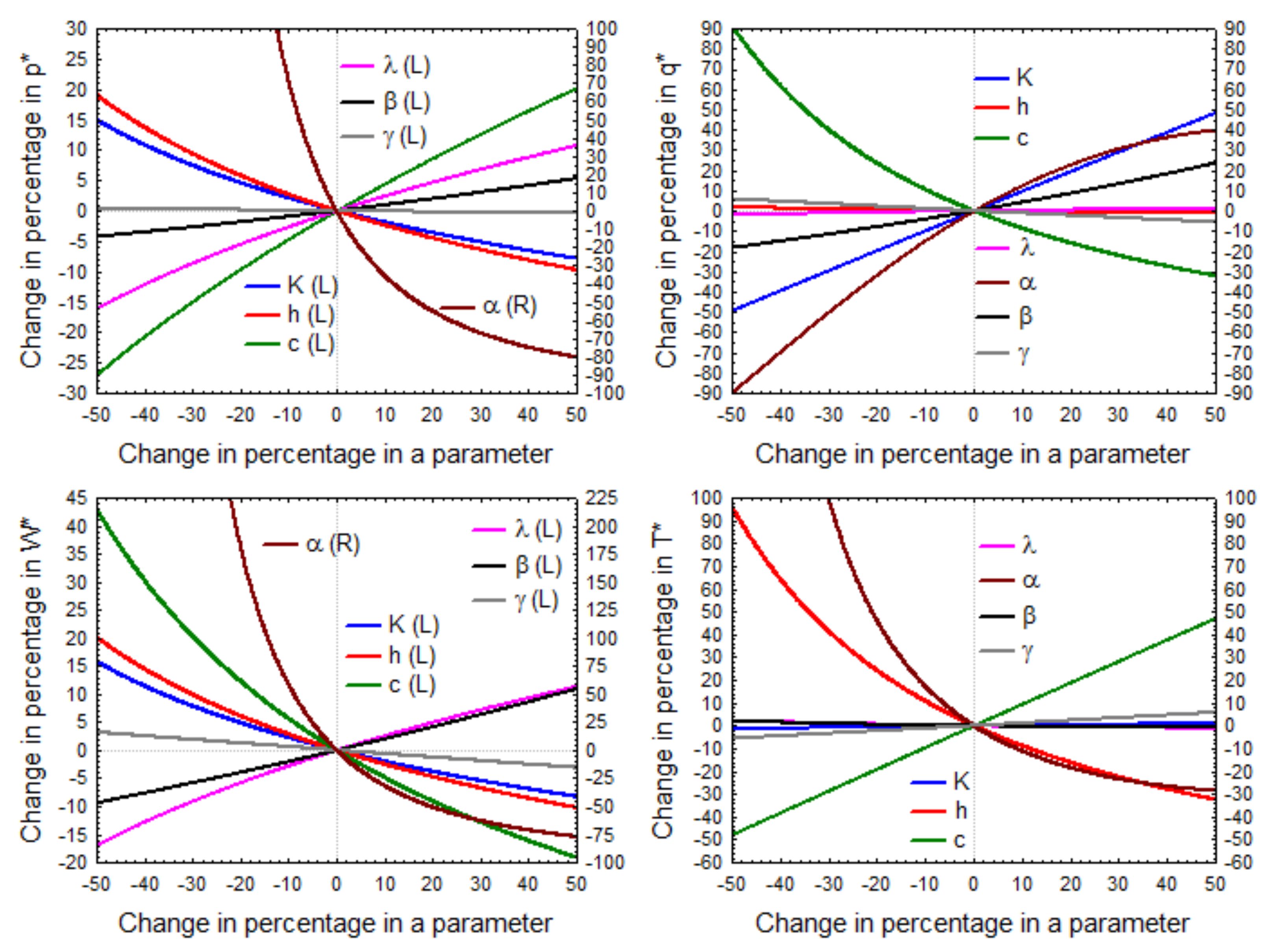
Now, to analyze the changes in percentage in the optimal policy regarding the initial parameters of the model, we have evaluated the optimal values for changes in percentage between $-50\%$ and $50\%$ in each of the parameters, keeping all the others fixed. The results are plotted in Figure 2.

The four graphs of Figure 2 illustrate how the parameter $\alpha$, and the different parameters K, h, $\lambda$, c, and $\gamma$, influence the optimal value of the selling price $p^{*}$, the profitability index $W^{*}$, the optimal lot size $q^{*}$, and the optimal cycle time $T^{*}$. The graphs corresponding to the optimal selling price $p^{*}$ and the profitability index $W^{*}$ are designed in the following way. As the changes in the parameter $\alpha$ are considerably more influential in $p^{*}$ and $W^{*}$ than the changes of the other parameters, these changes are plotted on the corresponding graphs, using a more detailed numerical scale marked in the right vertical axis (R). The other two graphs, corresponding to the optimal lot size $q^{*}$ and the optimal cycle time $T^{*}$, are designed drawing the influence of all the changes without different numerical scales. That is, although the changes in the parameter $\alpha$ are also more influential in $q^{*}$ and $T^{*}$ than the variations of the other parameters, all these changes are plotted on the corresponding graphs using the same numerical scale. This numerical scale is represented in both vertical axes (right axis (R) or left axis (L)).

After the $\alpha$ parameter, the unit purchasing cost c shows the largest changes in percentage in the optimal selling price $p^{*}$ and the maximum profitability index $W^{*}$. The rest of the parameters are less influential, and the trends are similar in both optimal values. Finally, the changes in percentage in the optimal lot size $q^{*}$ with respect to the ordering cost K, and the changes in percentage in the optimal cycle time $T^{*}$ related to the holding cost h per unit and per unit time, are also notable.

Next, to illustrate the results given in Section 5, the case of the isoelastic price-dependent demand rate has been considered by setting $\gamma =0$ in the previous numerical example. The optimal solutions have been evaluated with the expressions (29)–(32) given in Section 4. In addition, the basic case where the demand rate does not depend on the stock level, that is $\beta =\gamma =0$, has been evaluated with the expressions given in Table 2. The results for these optimal policies are collected in

Table 5. Maximum profitability policy in the models with isoelastic price-dependent demand.

	Selling Price ${\mathit{p}}_0^{*}$	Cycle Time ${\mathit{T}}_0^{*}$	Profitability Index ${\mathit{W}}_0^{*}$	Lot Size ${\mathit{q}}_0^{*}$
$\beta =0.2$ and $\gamma =0$	$41.82$	$4.09$	$1.1500$	$137.5$
$\beta =0$ and $\gamma =0$	$37.22$	4	$0.9306$	100
$\beta =0.2$ and $\gamma =3$	$47.62$	$4.58$	$1.2422$	$122.7$

. In order to compare results, the optimal values for the general case with $\beta =0.2$ and $\gamma =3$ have also been included. For this comparison, the value for the potential consumers has been kept at $\Lambda =300$, and the value of the scale parameter $\lambda$ has been recalculated with the new value $\gamma =0$. Specifically, $\lambda =300\times {20}^4=\mathrm{48,000,000}$. Note that, for the basic case with $\beta =\gamma =0$, the inventory model is not profitable because $W_0^{*}<1$.

To finish the computational results, the partial derivatives of the optimal solution concerning the parameters K, h, $\lambda$, and c of the model with isoelastic price-dependent demand ($\gamma =0$) and $\beta =0.2$, are evaluated with the expressions obtained in Section 5. From them, the absolute and relative rates of change in the optimal values for $p_0^{*}$, $T_0^{*}$, $W_0^{*}$, and $q_0^{*}$ were calculated. They are included in

Table 6. Absolute and relative rates of change in $p_0^{*}$, $q_0^{*}$, $W_0^{*}$, and $T_0^{*}$ with $\gamma =0$.

	$\mathit{x}=\mathit{K}=1000$	$\mathit{x}=\mathit{h}=5$	$\mathit{x}=\mathit{c}=20$	$\mathit{x}=\mathit{\lambda }=$ 48,000,000
$\partial p_0^{*}/\partial x$	$-0.0084$	$-2.09$	$0.94$	$0.000000021$
$\left(\partial p_0^{*}/\partial x\right)/\left(p_0^{*}/x\right)$	$-0.20$	$-0.25$	$0.45$	$0.25$
$\partial T_0^{*}/\partial x$	0	$0.82$	$-0.20$	0
$\left(\partial T_0^{*}/\partial x\right)/\left(T_0^{*}/x\right)$	0	1	$-1$	0
$\partial W_0^{*}/\partial x$	$-0.00023$	$-0.058$	$-0.032$	$0.000000006$
$\left(\partial W_0^{*}/\partial x\right)/\left(W_0^{*}/x\right)$	$-0.20$	$-0.25$	$-0.55$	$0.25$
$\partial q_0^{*}/\partial x$	$0.14$	0	$-6.88$	0
$\left(\partial q_0^{*}/\partial x\right)/\left(q_0^{*}/x\right)$	1	0	$-1$	0

.

Regarding the parameters K, h, $\lambda$, and c of the model, the unit purchasing cost c displays the largest relative rates of change for all the optimal values. Only the corresponding rates of change in the optimal cycle time $T_0^{*}$ with respect to the parameter h, and in the optimal lot size $q_0^{*}$ concerning the parameter K, equal the relative rates of change associated to the parameter c, but with opposite sign. In addition, the optimal cycle time $T_0^{*}$ does not depend on the parameters K nor $\lambda$, and the optimal lot size $q_0^{*}$ does not depend on the parameters h or $\lambda$. Finally, the respective effects of the parameters K, h, and $\lambda$ are equal in the optimal selling price $p_0^{*}$ and in the maximum profitability index $W_0^{*}$.

7. Conclusions and Future Research

This paper analyzes an inventory system with a broad frame for the demand rate. The joint effect of the selling price and the stock level on the demand is considered by using a potential function on both variables in a multiplicative way. The decision variables are the selling price, the depletion time, and the cycle time. The goal is the maximization of the profitability index, defined as the income/expense ratio in the inventory.

The inventory policy that maximizes the profit per unit time often requires high investment costs. In this case, the inventory manager perhaps prefers another policy with slightly less profit but much less expense. Thus, the solution with a maximum profitability index can be a more suitable option.

The optimal selling price can be obtained with a simple algorithm, which is easy to apply. The optimal depletion time is always equal to the optimal cycle time, i.e., the replacement must be done when the stock is depleted. The optimal values for the maximum profitability index, the cycle time, and the lot size can be evaluated in a closed-form from the optimal selling price. The optimal policy carries a proper balance between the ordering cost and the holding cost, which depends on the elasticity parameter of the demand corresponding to the stock level. The profitability of the inventory system can be assured by an inequality with the initial parameters.

For the special case of the model with isoelastic price-dependent demand, all optimal values are given with closed expressions. They only depend on the initial parameters. Moreover, they make it possible to establish, in a general way, the following managerial insights for the inventory managers:

(i)

The optimal values for the cycle time and the lot size do not depend on the scale parameter of the demand rate, which is defined by the number of potential customers per unit time.

(ii)

The optimal cycle time does not change if the ordering cost varies. Similarly, the optimal lot size does not change if the holding cost per unit and per unit time varies.

(iii)

An increase in the holding cost per unit and per unit time (keeping all the other parameters fixed) leads to a decrease in the optimal values for the selling price, the cycle time and the maximum profitability index.

(iv)

An increase in the ordering cost leads to an increase in the optimal values of the selling price and the lot size. On the other hand, it also leads to a decrease in the maximum profitability index.

(v)

An increase in the unit purchasing cost leads to an increase in the optimal values of the selling price and the cycle time. On the other hand, it also leads to a decrease in the optimal values of the lot size and the maximum profitability index.

(vi)

An increase in the scale parameter of the demand rate leads to an increase in the optimal values of the selling price and the maximum profitability index.

Regarding the relative effect of the parameters on the optimal values of the model with an isoelastic price-dependent demand, the following conclusions are drawn:

(i)

The maximum profitability index is equally sensitive regarding both, the scale parameter of the demand rate and the holding cost per unit and per unit time. However, it is less sensitive concerning the ordering cost. The sensitivity with respect to the unit purchasing cost can be greater or lower than regarding the parameters K, h, or $\lambda$, depending on the elasticity parameters of the demand rate with respect to the selling price and the stock level.

(ii)

In the same way, the optimal selling price is equally sensitive regarding both the scale parameter of the demand rate and the holding cost per unit and per unit time. However, it is less sensitive concerning the ordering cost. But now, the sensitivity with respect to the unit purchasing cost is always greater than regarding the parameters K, h, or $\lambda$.

(iii)

The optimal cycle time is equally sensitive with respect to the unit purchasing cost and the holding cost per unit and per unit time. As stated above, it does not depend on the scale parameter of the demand rate or the ordering cost.

(iv)

The optimal lot size is equally sensitive with respect to the unit purchasing cost and the ordering cost. As stated above, it does not depend on the scale parameter of the demand rate or the holding cost per unit and per unit time.

All these conclusions are based on the partial derivatives of the optimal policy with respect to the parameters of the model. Therefore, they can be completely generalized for all the practical applications of the model.

The closed expressions for all the optimal values have been also determined when the demand rate is isoelastic price-dependent and does not depend on the stock level.

Computational results show that the elasticity parameter of the demand rate regarding the selling price is the most influential parameter in the maximum profitability index and in the optimal selling price. Decreases of $15\%$ in this parameter can lead to increases of more than $100\%$ in the maximum profitability index or the optimal selling price.

Some possible extensions of the model that can be future research topics are: (i) to consider other functions for the demand rate; (ii) to suppose a non-linear holding cost; (iii) to incorporate discounts in the unit purchasing cost; (iv) to study the case of perishable or deteriorating items over time; and (v) to consider that the replenishment is not instantaneous, and there exists a replenishment period with a constant production rate.