Analytical Solutions of the Fractional Mathematical Model for the Concentration of Tumor Cells for Constant Killing Rate

Abstract

Two generalized mathematical models with memory for the concentration of tumor cells have been analytically studied using the cylindrical coordinate and the integral transform methods. The generalization consists of the formulating of two mathematical models with Caputo-time fractional derivative, models that are suitable to highlight the influence of the history of tumor evolution on the present behavior of the concentration of cancer cells. The time-oscillating concentration of cancer cells has been considered on the boundary of the domain. Analytical solutions of the fractional differential equations of the mathematical models have been determined using the Laplace transform with respect to the time variable and the finite Hankel transform with respect to the radial coordinate. The positive roots of the transcendental equation with Bessel function $J_0(r)=0$, which are needed in our study, have been determined with the subroutine $r_n=root(J_0(r),r,(2n-1)\pi /4,(2n+3)\pi /4),n=1,2,\dots$ of the Mathcad 15 software. It is found that the memory effects are stronger at small values of the time, t. This aspect is highlighted in the graphical illustrations that analyze the behavior of the concentration of tumor cells. Additionally, the concentration of cancer cells is symmetric with respect to radial angle, and its values tend to be zero for large values of the time, t.

1. Introduction

Cancer is the world’s second most common cause of death and is responsible for an estimated 9.6 million deaths per year. One of the most useful and inexpensive approaches to determine and predict the stage, size, and growth of a cancer tumor as a reaction of the diffusion process is the mathematical modeling.

The problem of growth of glioma, a kind of brain tumor, has been modeled based upon tumor cell diffusion coupled with growth rate by Cook et al. [1], Tracqui et al. [2], and Woodward et al. [3], who incorporated the two most important processes in the growth of brain tumors, namely, the proliferation of cells and the diffusion process, resulting in a reaction diffusion equation.

A generalized diffusion-based cancer tumor model has been described by Burgess et al. [4]:

$$u_t={\nabla }^2(Du)+pu-ku$$

(1)

where $u(r,t)$ is cell concentration at time, $t$, and radius, $r$ (in 3-D space), ${\nabla }^2$ is the Laplacian operator, $p$ is the rate of growth of the cell (proliferation rate of cell), $k$ is the killing rate of the cell, and $D$ is the diffusion coefficient.

Moyo and Leach [5] suggested a governing equation of the cancer tumor model with a $K(x,t)=p-k$ variable killing rate, namely:

$$u_t=u_{xx}-K(x,t)u$$

(2)

where the cancer tumor cell concentration is $u(x,t)$.

Some exact solutions of the previous equations have been determined by the authors using Lie symmetry analysis. Bokhari et al. [6] have employed the Lie symmetry analysis method to obtain some exact solutions and conservation laws for killing rate, dependent on tumor cell density.

A mathematical model for glioblastomas (a highly invasive glioma in the brain) has been described by Murray [4], which includes the two main parameters of tumor growth, namely the diffusion of cancer cells and the rate of cell proliferation. The solution to the model equation based on patient parameters of tumor growth illustrates why certain patients remain alive after identical prescription medications, specifically surgical resection (removal) and radiation exposure.

In all the above models, the diffusion of the cell has been considered as the time rate of change of the cell density. It is well understood that, in many cases, the best description of the model may be the assumption of fractional diffusion.

Fractional (non-integer order) calculus can provide a succinct model to better explain some dynamic events. The fractional calculus is successfully applied in physics, chemistry, biology, and materials science to describe dielectrics, viscoelastic materials, and many transport processes. The fractional calculus with Caputo differential operators [7,8] has been widely used in many fields of science and engineering over the last few decades. Caputo amends Darcy’s law by adding a formalism of memory, defined by the time-fractional derivatives.

Iomin [9] has investigated the influence of cell fission on the transport properties of the vessel network and developed a mathematical model based on the heuristic arguments on tumor development. The constructed model is a modification of the so-called comb structure. In the framework of this model, the author proved that the tumor development corresponds to the fractional transport of cells. This model could also be a possible mechanism for diffusive cancers.

A model of the cancer tumor based on the fractional time-derivative has been investigated by Iyiola and Zaman [10] using the q-homotopy analysis method. They have determined approximate series solutions for the various considered cases. The conclusion drawn from the research carried out in their paper is that the therapy-dependent killing rate, K, does not only need to be a function of time, or of both, position and time, but can also depend on the cancer cell concentration.

The purpose of this article is to investigate two mathematical models regarding the cylindrical coordinate of the cancerous tumor in which the concentration of the cancer cells is time-dependent and also dependent on the radial coordinate.

Further, mathematical models are based on the time-fractional Caputo derivative, which involves a power-law of the memory kernel (See Appendix A, Equation (A6)). The fractional partial differential equations of the mathematical models are:

$$\frac{{\partial }^{\alpha }u(r,t)}{\partial t^{\alpha }}=D\frac{1}{r}\frac{\partial }{\partial r}\left(r\frac{\partial u(r,t)}{\partial r}\right)-Ku(r,t),\hspace{0.17em}\hspace{0.17em}\hspace{0.17em}t\ge 0,\hspace{0.17em}\hspace{0.17em}r\in (0,1)$$

(3)

and

$$\frac{{\partial }^{\alpha }u(r,\theta ,t)}{\partial t^{\alpha }}=D\frac{1}{r}\frac{\partial }{\partial r}\left(r\frac{\partial u(r,\theta ,t)}{\partial r}\right)+\frac{{\partial }^{2}u(r,\theta ,t)}{\partial {\theta }^2}-Ku(r,\theta ,t),\hspace{0.17em}t\ge 0,\hspace{0.17em}r\in (0,1),\hspace{0.17em}\theta \in (0,2\pi )$$

(4)

In the considered models, the diffusion parameter, D, and the killing rate of cells, $K$, are assumed to be constant. The solutions to the problems are obtained using the Laplace transform and the finite Hankel transform under appropriate initial and boundary conditions.

The effects of the memory parameter, as well as time, on the tumor cell concentration, $u$, are studied by numerical calculations and graphical illustrations obtained with the Mathcad software.

2. Solution of the Problems

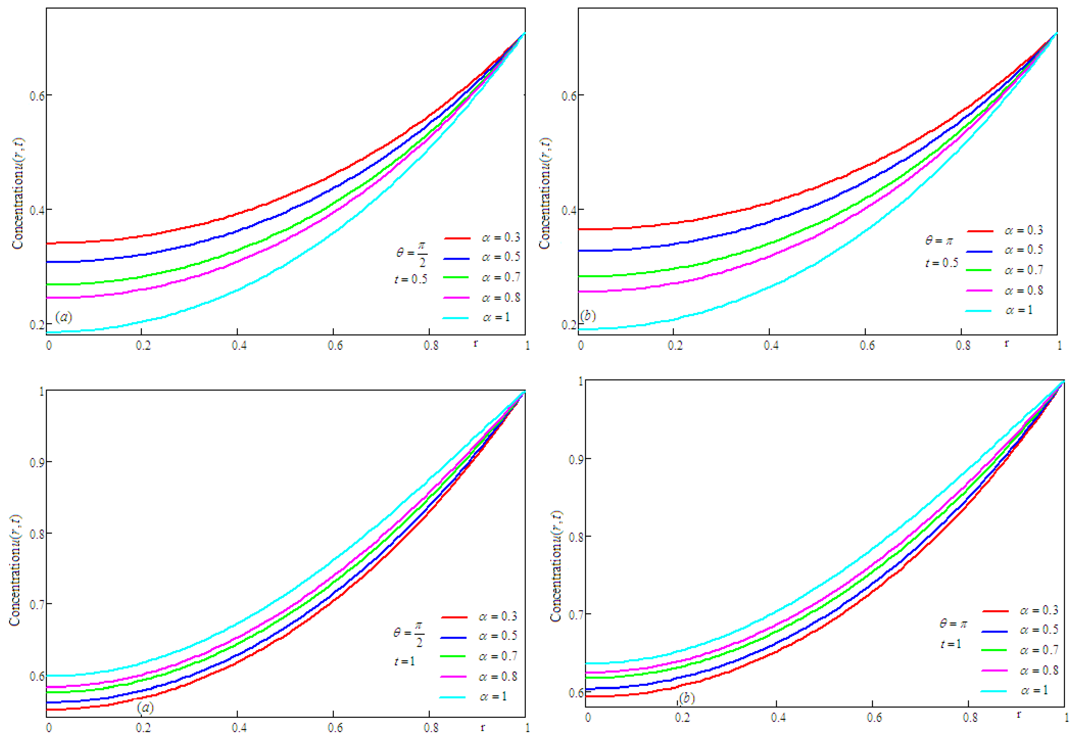
2.1. The Concentration of Tumor Cells $u(r,t)$

The generalized concentration of tumor cells $u(r,t)$ given by Equation (3) will be determined under the following initial and boundary conditions:

$$u(r,0)=0,\hspace{0.17em}r\in [0,1]$$

(5)

$$u(1,t)=H(t)e^{i\omega t},\hspace{0.17em}\hspace{0.17em}t\ge 0$$

(6)

To determine the analytical solution of Equation (3) with the initial and boundary conditions (5) and (6), the Laplace transform with respect to the variable, t, and the finite Hankel transform with respect to the radial coordinate, r, will be used.

Applying the Laplace transform to Equation (3) and using the initial condition (5), we obtain the transformed equation:

$$s^{\alpha }\overline{u}(r,s)=D\frac{1}{r}\frac{\partial }{\partial r}\left(r\frac{\partial \overline{u}(r,s)}{\partial r}\right)-K\overline{u}(r,s)$$

(7)

where $\overline{u}(r,s)={\displaystyle \underset{0}{\overset{\infty }{\int }}u(r,t)e^{-st}dt}$ denotes the Laplace transform of function $u(r,t)$ [11].

The transformed function $\overline{u}(r,s)$ has to satisfy the boundary condition:

$$\overline{u}(1,s)=\frac{1}{s-i\omega }$$

(8)

Applying the finite Hankel transform [12,13] to Equation (7) and using Equation (8), we get:

$$\begin{array}{l}{\overline{u}}_H(r_n,s)=\frac{D{r}_n}{(s-i\omega )(s^{\alpha }+D{r}_n^2+K)}{J}_1(r_n)=\\ \hspace{1em}\hspace{1em}\hspace{1em}\hspace{1em}\frac{J_1(r_n)}{r_n(s-i\omega )}-\frac{J_1(r_n)}{r_n(s-i\omega )}{\overline{F}}_n(s),\hspace{0.17em}{\overline{F}}_n(s)=\frac{s^{\alpha }+K}{s^{\alpha }+D{r}_n^2+K}.\end{array}$$

(9)

where $r_n,\hspace{0.17em}\hspace{0.17em}n=1,2,3\dots$ are the positive roots of the transcendental equation $J_0(r)=0$ and ${\overline{u}}_H(r_n,s)={\displaystyle \underset{0}{\overset{1}{\int }}r\hspace{0.17em}\overline{u}(r,s)J_0(r{r}_n)dr}$ denotes the finite Hankel transform of the function $\overline{u}(r,s)$, whose inverse transform is given by (Appendix A, Equation (A11)):

$$\overline{u}(r,s)=2{\displaystyle \sum _{n=1}^{\infty }\frac{J_0(r{r}_n)}{J_1^2(r_n)}{\overline{u}}_H(r_n,s)}$$

(10)

In the above relations, $\hspace{0.17em}{J}_{\alpha }(\cdot )$ is the Bessel function of the first kind and order, $\hspace{0.17em}\alpha$.

To determine the inverse Laplace transform and the inverse Hankel transform of the function given by Equation (9), we use (10) and the formula:

$$L^{-1}\left\{\frac{s^{\alpha -\beta }}{s^{\alpha }-b}\right\}=t^{\beta -1}{E}_{\alpha ,\beta }(b{t}^{\alpha }),\hspace{0.17em}\hspace{0.17em}{E}_{\alpha ,\beta }(z)={\displaystyle \sum _{k=o}^{\infty }\frac{z^k}{\mathsf{\Gamma }(\alpha k+\beta )},\hspace{0.17em}\mathrm{Re}(\alpha )>0},\hspace{0.17em}\mathrm{Re}(\beta )>0\hspace{0.17em}\hspace{0.17em}$$

(11)

where $\hspace{0.17em}{E}_{\alpha ,\beta }(z)$ is the Mittage–Leffler function [14].

Using the above relations and the auxiliary function $f(r)=1$, whose finite Hankel transform is:

$$\hspace{0.17em}{f}_H(r_n)=\frac{J_1(r_n)}{r_n},\hspace{0.17em}\hspace{0.17em}$$

(12)

we obtain the generalized concentration of cancer cell given by:

$$u(r,t)=e^{i\omega t}-2{\displaystyle \sum _{n=1}^{\infty }{F}_n(t)\frac{J_0(r{r}_n)}{r_n{J}_1(r_n)}}$$

(13)

where

$$F_n(t)=E_{\alpha ,1}(-a_n{t}^{\alpha })+{\displaystyle \underset{0}{\overset{t}{\int }}{e}^{i\omega (t-\tau )}\left[i\omega E_{\alpha ,1}(-a_n{\tau }^{\alpha })+K{E}_{\alpha ,\alpha }(-a_n{\tau }^{\alpha })\right]}d\tau$$

(14)

and $a_n=D{r}_n^2+K,\hspace{0.17em}\hspace{0.17em}n=1,2,3\dots$.

For $\alpha =1$, the concentration cells (13) has the simpler form:

$$u(r,t)=e^{i\omega t}-{\displaystyle \sum _{n=1}^{\infty }\left(\frac{K+i\omega }{a_n+i\omega }{e}^{i\omega t}-\frac{a_n-K}{a_n+i\omega }{e}^{-a_{n}t}\right)}\frac{J_0(r{r}_n)}{r_n{J}_1(r_n)}$$

(15)

Figure 1 and Figure 2 have been plotted to highlight the influence of the memory parameter, α, on the concentration of the tumor cells. These figures are presented for different values of the fractional parameter, α, at four values of time, t, namely $t\in \{0.5,\hspace{0.17em}1,\hspace{0.17em}15,\hspace{0.17em}20\}$. Figure 1 corresponds to the sine-variation of concentration $u(1,t)$ and Figure 2 corresponds to the cosine-variation of the concentration $u(1,t)$. It can be observed that, for large values of time, t, the values of concentration $u(r,t)$ are of the order ${10}^{-4}-{10}^{-3}$, and the influence of the fractional parameter is insignificant. This behavior is due to the evolution in time of the Caputo kernel $h_C(t,\alpha )=\frac{t^{-\alpha }}{\mathsf{\Gamma }(1-\alpha )},\hspace{0.17em}0<\alpha <1$, which has small values for large amounts of time; therefore, the damping of the rate of concentration is negligible. For this reason, the influence of the fractional parameter is insignificant for large values of time, t. However, for small values of time, t, the values of the Caputo kernel have a significant influence on the rate of concentration. In this case, the memory of the diffusion process has a significant influence on the concentration of tumor cells. It is easily seen that a diffusion process with small values of the memory parameter leads to a smaller concentration of the tumor cells in the case of short time of treatment.

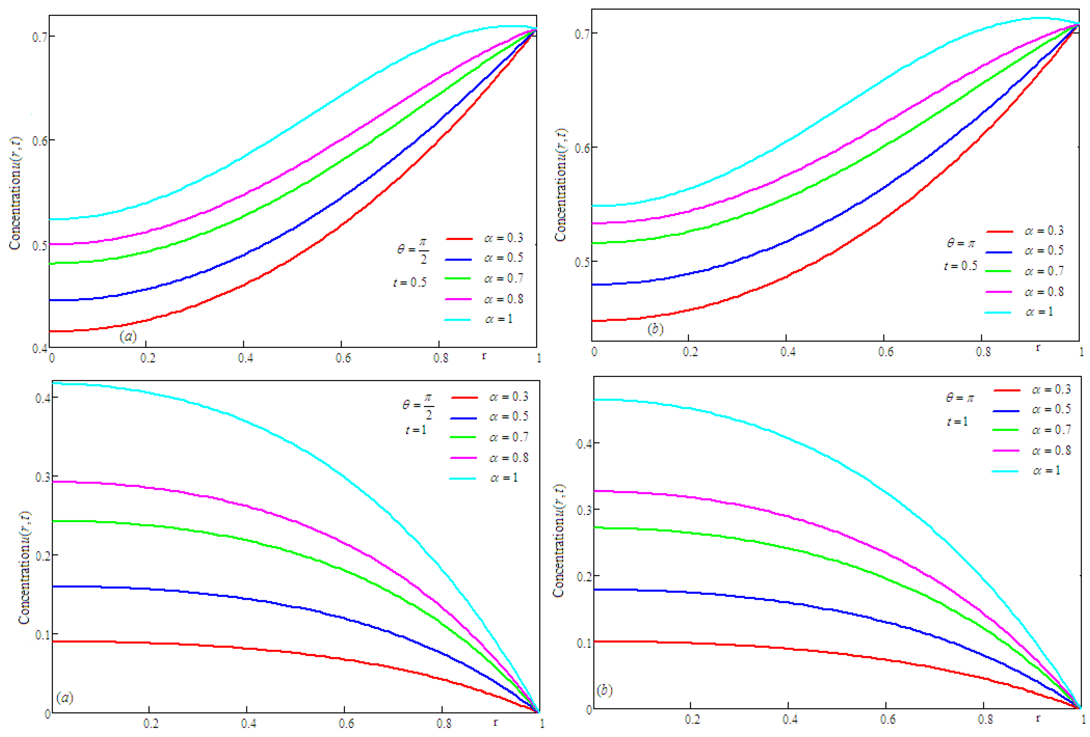
2.2. The Concentration of Tumor Cells $u(r,\theta ,t)$

This section deals with the findings of the solution of the fractional differential Equation (4), along with the initial and boundary conditions:

$$u(r,\theta ,0)=0,\hspace{0.17em}\hspace{0.17em}r\in [0,1],\hspace{0.17em}\theta \in [0,2\pi ]$$

(16)

$$u(1,\theta ,t)=H(t)e^{i\omega t},\hspace{0.17em}\hspace{0.17em}t>0,\hspace{0.17em}\theta \in (0,2\pi )$$

(17)

$$u(r,0,t)=u(r,2\pi ,t)=0,\hspace{0.17em}t>0,\hspace{0.17em}r\in (0,1)$$

(18)

Applying the Laplace transform to Equation (4) and using the initial condition (16), we obtain the transformed equation:

$$s^{\alpha }\overline{u}(r,\theta ,t)=D\frac{1}{r}\frac{\partial }{\partial r}\left(r\frac{\partial \overline{u}(r,\theta ,s)}{\partial r}\right)+\frac{{\partial }^2\overline{u}(r,\theta ,s)}{\partial {\theta }^2}-K\overline{u}(r,\theta ,s)$$

(19)

where $\overline{u}(r,\theta ,s)={\displaystyle \underset{0}{\overset{\infty }{\int }}u(r,\theta ,t)e^{-st}dt}$ is the Laplace transform of function $u(r,\theta ,t)$.

The function $\overline{u}(r,\theta ,s)$ has to satisfy the boundary conditions:

$$\begin{array}{l}\overline{u}(1,\theta ,s)=\frac{1}{s-i\omega },\theta \in (0,2\pi ),\\ \overline{u}(r,0,s)=\overline{u}(r,2\pi ,s)=0,\hspace{0.17em}r\in (0,1).\end{array}$$

(20)

Applying the finite Hankel transform to Equation (19) and using Equation (20), we obtain the differential equation:

$$\frac{{\partial }^2{\overline{u}}_H(r_n,\theta ,s)}{\partial {\theta }^2}-(s^{\alpha }+D{r}_n^2+K){\overline{u}}_H(r_n,\theta ,s)+\frac{D{r}_n{J}_1(r_n)}{s-i\omega }=0$$

(21)

where $r_n,\hspace{0.17em}n=1,2,3\dots$ are the positive roots of the transcendental Equation $J_0(r)=0$ and ${\overline{u}}_H(r_n,\theta ,s)={\displaystyle \underset{0}{\overset{1}{\int }}r\overline{u}(r,\theta ,s)J_0(r{r}_n)dr}$ is the finite Hankel transform of the function $\overline{u}(r,\theta ,s)$.

The general solution of Equation (21) is:

$${\overline{u}}_H(r_n,\theta ,s)=C_1{e}^{\theta \sqrt{s^{\alpha }+a_n}}+C_2{e}^{-\theta \sqrt{s^{\alpha }+a_n}}+\frac{D{r}_n{J}_1(r_n)}{(s-i\omega )(s^{\alpha }+a_n)}$$

(22)

where $a_n=D{r}_n^2+K,\hspace{0.17em}\hspace{0.17em}n=1,2,3\dots$.

Using the boundary conditions (20), we obtain for the transformed velocity the form:

$$\begin{array}{l}{\overline{u}}_H(r_n,\theta ,s)=\frac{D{r}_n{J}_1(r_n)}{(s-i\omega )(s^{\alpha }+a_n)}\frac{\left(e^{-2\pi \sqrt{s^{\alpha }+a_n}}-1\right)e^{\theta \sqrt{s^{\alpha }+a_n}}}{e^{2\pi \sqrt{s^{\alpha }+a_n}}-e^{-2\pi \sqrt{s^{\alpha }+a_n}}}+\frac{D{r}_n{J}_1(r_n)}{(s-i\omega )(s^{\alpha }+a_n)}\frac{\left(1-e^{2\pi \sqrt{s^{\alpha }+a_n}}\right)e^{-\theta \sqrt{s^{\alpha }+a_n}}}{e^{2\pi \sqrt{s^{\alpha }+a_n}}-e^{-2\pi \sqrt{s^{\alpha }+a_n}}}+\\ \hspace{0.17em}\hspace{0.17em}\hspace{0.17em}\hspace{0.17em}\hspace{0.17em}\hspace{0.17em}\hspace{0.17em}\hspace{0.17em}\hspace{0.17em}\hspace{0.17em}\hspace{0.17em}\hspace{0.17em}\hspace{0.17em}\hspace{0.17em}\hspace{0.17em}\hspace{0.17em}\hspace{0.17em}\hspace{0.17em}\hspace{0.17em}\hspace{0.17em}\hspace{0.17em}\hspace{0.17em}\hspace{0.17em}\hspace{0.17em}\hspace{0.17em}\hspace{0.17em}\hspace{0.17em}\hspace{0.17em}\hspace{0.17em}\hspace{0.17em}\hspace{0.17em}\hspace{0.17em}\hspace{0.17em}\hspace{0.17em}\hspace{0.17em}\hspace{0.17em}\hspace{0.17em}\hspace{0.17em}\hspace{0.17em}\hspace{0.17em}\hspace{0.17em}\hspace{0.17em}\hspace{0.17em}\hspace{0.17em}\hspace{0.17em}\hspace{0.17em}\hspace{0.17em}\hspace{0.17em}\hspace{0.17em}\hspace{0.17em}\hspace{0.17em}\hspace{0.17em}\hspace{0.17em}\hspace{0.17em}\hspace{0.17em}\hspace{0.17em}\hspace{0.17em}+\frac{D{r}_n{J}_1(r_n)}{(s-i\omega )(s^{\alpha }+a_n)}.\end{array}$$

(23)

Let $w_1(s)=\sqrt{s^{\alpha }+a_n}$ and, using the expansion $\frac{1}{1-e^{-4\pi w_1(s)}}={\displaystyle \sum _{k=0}^{\infty }{e}^{-4\pi k{w}_1(s)}}$, we obtain:

$${\overline{u}}_H(r_n,\theta ,s)=\frac{J_1(r_n)}{r_n(s-i\omega )}-F_n(s)\frac{J_1(r_n)}{r_n}+\frac{D{r}_n{J}_1(r_n)}{(s-i\omega )}{G}_n(s)$$

(24)

where:

$$F_n(s)=\frac{s^{\alpha }+K}{(s-i\omega )(s^{\alpha }+a_n)}$$

(25)

$$G_n(s)={\displaystyle \sum _{k=0}^{\infty }\left[\frac{e^{-(4k\pi +4\pi -\theta )\sqrt{s^{\alpha }+a_n}}}{s^{\alpha }+a_n}-\frac{e^{-(4k\pi +2\pi -\theta )\sqrt{s^{\alpha }+a_n}}}{s^{\alpha }+a_n}+\frac{e^{-(4k\pi +2\pi +\theta )\sqrt{s^{\alpha }+a_n}}}{s^{\alpha }+a_n}-\frac{e^{-(4k\pi +\theta )\sqrt{s^{\alpha }+a_n}}}{s^{\alpha }+a_n}\right]}$$

(26)

Applying the inverse Hankel transform to Equation (25), we have:

$$\overline{u}(r,\theta ,s)=\frac{1}{s-i\omega }-2{\displaystyle \sum _{n=1}^{\infty }{F}_n(s)\frac{J_0(r{r}_n)}{r_n{J}_1(r_n)}}+2{\displaystyle \sum _{n=1}^{\infty }\frac{D{r}_n{J}_0(r{r}_n)}{J_1(r_n)}}\frac{G_n(s)}{s-i\omega }$$

(27)

To determine the inverse Laplace transform of $G_n(s)$, we consider the auxiliary function $H(s)=\frac{e^{-a\sqrt{s}}}{s}$, whose inverse Laplace transform is $h(t)=\mathrm{erfc}\left(\frac{a}{2\sqrt{t}}\right)$, $\mathrm{erfc}(\cdot )$ being the complementary error function. Let $w(s),\hspace{0.17em}{H}_1(s)$ be the functions $w(s)=s^{\alpha }+a_n$ and $H_1(s)=\frac{e^{-z\sqrt{s^{\alpha }+a_n}}}{s^{\alpha }+a_n}$.

It is easy to see that $H_1(s)=H(w(s))$, and therefore, $L^{-1}\{H_1(s)\}={\displaystyle \underset{0}{\overset{\infty }{\int }}h(y)\psi (t,y)dy}$,

where $\psi (t,y)=L^{-1}\left\{e^{-yw(s)}\right\}=L^{-1}\left\{e^{-y{a}_n}{e}^{-y{s}^{\alpha }}\right\}=\{\begin{array}{l}{e}^{-y{a}_n}\varphi (0,-\alpha ,-y{t}^{-\alpha }),\hspace{0.17em}\hspace{0.17em}\hspace{0.17em}0<\alpha <1,\\ e^{-y{a}_n}\delta (t-y),\hspace{0.17em}\hspace{0.17em}\hspace{0.17em}\hspace{0.17em}\hspace{0.17em}\hspace{0.17em}\hspace{0.17em}\hspace{0.17em}\hspace{0.17em}\hspace{0.17em}\hspace{0.17em}\hspace{0.17em}\hspace{0.17em}\hspace{0.17em}\hspace{0.17em}\hspace{0.17em}\hspace{0.17em}\hspace{0.17em}\hspace{0.17em}\hspace{0.17em}\alpha =1.\end{array}$.

In the above relationship, $\varphi (0,-\alpha ,-y{t}^{-\alpha })$ is the Wright function [15], which satisfies the property $t^{\beta -1}\varphi (\beta ,-\alpha ,-y{t}^{-\alpha })=L^{-1}\left\{\frac{1}{s^{\beta }}{e}^{-y{s}^{\alpha }}\right\},\hspace{0.17em}\hspace{0.17em}0<\alpha <1$, and $\delta (\cdot )$ is Dirac’s distribution.

Finally, we get the solution:

$$u(r,\theta ,t)=e^{i\omega t}-2{\displaystyle \sum _{n=1}^{\infty }{f}_n(t)\frac{J_0(r{r}_n)}{J_1(r_n)}}+2{\displaystyle \sum _{n=1}^{\infty }\frac{D{r}_n{J}_0(r{r}_n)}{J_1(r_n)}}{\displaystyle \underset{0}{\overset{t}{\int }}{e}^{i\omega (t-\tau )}{g}_n(\tau )d\tau }$$

(28)

where:

$$f_n(t)=L^{-1}\{F(s)\}=E_{\alpha ,1}(-a_n{t}^{\alpha })+{\displaystyle \underset{0}{\overset{t}{\int }}{e}^{i\omega (t-\tau )}}\left[i\omega E_{\alpha ,1}(-a_n{\tau }^{\alpha })+K{\tau }^{\alpha -1}{E}_{\alpha ,\alpha }(-a_n{\tau }^{\alpha })\right]d\tau$$

(29)

$$g_n(t)={\displaystyle \sum _{k=0}^{\infty }{\displaystyle \underset{0}{\overset{\infty }{\int }}\begin{array}{l}\left[\mathrm{erfc}\left(\frac{4k\pi +4\pi -\theta }{2\sqrt{y}}\right)-\mathrm{erfc}\left(\frac{4k\pi +2\pi -\theta }{2\sqrt{y}}\right)+\mathrm{erfc}\left(\frac{4k\pi +2\pi +\theta }{2\sqrt{y}}\right)-\mathrm{erfc}\left(\frac{4k\pi +\theta }{2\sqrt{y}}\right)\right]\times \\ \hspace{0.17em}\hspace{0.17em}\hspace{0.17em}\hspace{0.17em}\hspace{0.17em}\hspace{0.17em}\hspace{0.17em}\hspace{0.17em}\hspace{0.17em}\hspace{0.17em}\hspace{0.17em}\hspace{0.17em}\hspace{0.17em}\hspace{0.17em}\hspace{0.17em}\hspace{0.17em}\hspace{0.17em}\hspace{0.17em}\hspace{0.17em}\hspace{0.17em}\hspace{0.17em}\hspace{0.17em}\hspace{0.17em}\hspace{0.17em}\hspace{0.17em}\hspace{0.17em}\hspace{0.17em}\hspace{0.17em}\hspace{0.17em}\hspace{0.17em}\hspace{0.17em}\hspace{0.17em}\hspace{0.17em}\hspace{0.17em}\hspace{0.17em}\hspace{0.17em}\hspace{0.17em}\hspace{0.17em}\hspace{0.17em}\hspace{0.17em}\hspace{0.17em}\hspace{0.17em}\hspace{0.17em}\hspace{0.17em}\hspace{0.17em}\hspace{0.17em}\hspace{0.17em}\hspace{0.17em}\hspace{0.17em}\hspace{0.17em}\hspace{0.17em}\hspace{0.17em}\hspace{0.17em}\hspace{0.17em}\hspace{0.17em}\hspace{0.17em}\hspace{0.17em}\hspace{0.17em}\hspace{0.17em}\hspace{0.17em}\hspace{0.17em}\hspace{0.17em}\hspace{0.17em}\hspace{0.17em}\hspace{0.17em}\hspace{0.17em}\hspace{0.17em}\hspace{0.17em}\hspace{0.17em}\hspace{0.17em}\hspace{0.17em}\hspace{0.17em}\hspace{0.17em}\hspace{0.17em}\hspace{0.17em}\hspace{0.17em}\hspace{0.17em}\hspace{0.17em}\hspace{0.17em}\hspace{0.17em}\hspace{0.17em}\hspace{0.17em}\hspace{0.17em}\times e^{-a_{n}y}{t}^{-1}\varphi \left(0,-\alpha ,-y{t}^{-\alpha }\right)dy,\hspace{0.17em}\hspace{0.17em}\hspace{0.17em}\hspace{0.17em}0<\alpha <1.\end{array}}}$$

(30)

For $\alpha =1$, the functions $f_n(t),\hspace{0.17em}{g}_n(t)$ have the simpler expressions:

$$\begin{array}{l}{f}_n(t)=\frac{1}{a_n+i\omega }\left[(K+i\omega )e^{i\omega t}+D{r}_n^2{e}^{-a_{n}t}\right],\\ g_n(t)={\displaystyle \sum _{k=0}^{\infty }\left[\mathrm{erfc}\left(\frac{4k\pi +4\pi -\theta }{2\sqrt{t}}\right)-\mathrm{erfc}\left(\frac{4k\pi +2\pi -\theta }{2\sqrt{t}}\right)\right]}{e}^{-a_{n}t}+\\ \hspace{1em}\hspace{1em}\hspace{1em}{\displaystyle \sum _{k=0}^{\infty }\left[\mathrm{erfc}\left(\frac{4k\pi +2\pi +\theta }{2\sqrt{t}}\right)-\mathrm{erfc}\left(\frac{4k\pi +\theta }{2\sqrt{t}}\right)\right]}{e}^{-a_{n}t}.\\ \end{array}$$

(31)

Based on Equation (28), the evolution in space and in time of the concentration of cancer cells, as well as the influence of the memory parameter on its evolution, have been analyzed and presented in graphs in Figure 3, Figure 4 and Figure 5. The cases of sinusoidal and co-sinusoidal variation of $u(r,\theta ,t)$ concentration were considered.

Figure 3 and Figure 4 present the profiles of concentration of tumor cells versus the radial angle, $\theta$, for the fractional parameter $\alpha =0.5$ at the instant $t=0.5$. As expected, the profiles of concentration are symmetric with respect to the radial angle due to equal boundary conditions in the positions $\theta =0,\hspace{0.17em}\theta =2\pi$. Additionally, Figure 3 and Figure 4 show the variation of the concentration of tumor cells with the radial coordinate, r. As can be seen in Figure 3 and Figure 4, for the considered case, the concentration is increasing with the radial distance, r.

Figure 5 and Figure 6 have been plotted to highlight the influence of the fractional parameter, $\alpha$, on the concentration of tumor cells. These figures present profiles of the concentration $u(r,\theta ,t)$ versus r for different values of the memory parameter at small values of time, t. It can be observed in Figure 5 and Figure 6 that, for small values of time, the memory effects are stronger. This behavior is due to the time-evolution of the Caputo kernel, which, for small amounts of time, has bigger values, therefore the influence on the rate of concentration will be stronger.

The time variation of the tumor cell concentration is shown in Figure 7 and Figure 8 for different values of the α fractional parameter. The graphs in Figure 7 and Figure 8 were drawn for the spatial positions $r=0.2,\hspace{0.17em}\theta \in \{\pi /2,\hspace{0.17em}\pi \}$ and $r=0.4,\hspace{0.17em}\theta \in \{\pi /2,\hspace{0.17em}\pi \}$, for $K=1,\hspace{0.17em}D=0.5$ and $\omega =\pi /20$, respectively. In Figure 7 are plotted the concentration profiles for the boundary condition $u(1,\theta ,t)=\sin (\omega t)$, while Figure 8 presents the case corresponding to $u(1,\theta ,t)=\cos (\omega t)$. In both cases, the influence of the memory parameter is different for small values of time, t, and for large values of time, t; namely, for small values of the time, t, the concentration is decreasing with the fractional parameters and has the opposite behavior for large values of the time, t.

For large values of the time, t, the concentration of tumor cells tends to be zero. This property is obtained graphically, but it is obvious from Equation (22), along with the property $\underset{t\to \infty }{\lim }f(t)=\underset{s\to 0}{\lim }s\hspace{0.17em}L\left\{f(t)\right\}$.

3. Conclusions

Two generalized mathematical models for the concentration of tumor cells have been analytically studied by using the integral transform method.

The generalization consists of the development of mathematical models with Caputo-time fractional derivatives that are suitable for highlighting the memory effects.

Cylindrical coordinate has been employed in our study, and the time-oscillating concentration of cancer cells on the boundary $r=1$ has been considered.

Analytical solutions of the fractional differential equations of the mathematical models have been determined using the Laplace transform with respect to the time variable and the finite Hankel transform with respect to the radial coordinate, r.

The positive roots of the transcendental equation with Bessel function $J_0(r)=0$, which are needed in our study, have been determined with the subroutine $r_n=root(J_0(r),r,(2n-1)\pi /4,(2n+3)\pi /4),n=1,2,\dots$ of the Mathcad 15 software.

Because the Caputo kernel has the power-law form, namely $h_C(t,\alpha )=\frac{t^{-\alpha }}{\mathsf{\Gamma }(1-\alpha )},\hspace{0.17em}0<\alpha <1$, the memory effects are stronger at small values of time, t. This aspect is highlighted in the graphical illustrations, which analyze the behavior of the concentration of tumor cells.

It is found that concentration of cancer cells is symmetric with respect to the radial angle, and its values tend to be zero for large values of time, t.

References

1. Cook, J.; Woodward, D.E.; Tracqui, P.; Murray, J.D. Resection of gliomas and life expectancy. J. Neuro Oncol. 1995, 24, 131–135. [Google Scholar]
2. Tracqui, P.; Cruywagen, G.C.; Woodward, D.E.; Bartoo, G.T.; Murray, J.D.; Alvord, E.C. A mathematical model of glioma growth: The effect of chemotherapy on spatio-temporal growth. Cell Prolif. 1995, 28, 17–31. [Google Scholar] [CrossRef] [PubMed]
3. Woodward, D.E.; Cook, J.; Tracqui, P. A mathematical model of glioma growth, The effect of extent of surgical resection. Cell Prolif. 1996, 26, 269–288. [Google Scholar] [CrossRef] [PubMed]
4. Burgess, P.K.; Kulesa, P.M.; Murray, J.D.; Alvord, E.C. The interaction of growth rates and diffusion coefficients in a three-dimensional mathematical model of gliomas. J. Neuropathol. Exper. Neurol. 1997, 56, 704–713. [Google Scholar] [CrossRef]
5. Moyo, S.; Leach, P.G.L. Symmetry methods applied to a mathematical model of a tumor of the brain. Proc. Inst. Math. NAS Ukr. 2004, 50, 204–210. [Google Scholar]
6. Bokhari, A.; Kara, A.; Zaman, F. On the solutions and conservation laws of the model for tumor growth in the brain. J. Math. Anal. Appl. 2009, 350, 256–261. [Google Scholar] [CrossRef] [Green Version]
7. Podlubny, I. Fractional Differential Equations, Mathematics in Science and Engineering; Academic Press: San Diego, CA, USA, 1999. [Google Scholar]
8. Hristov, J. Bio-Heat Models Revisited: Concepts, Derivations, Nondimensalization and Fractionalization Approaches. Front. Phys. 2019, 7. [Google Scholar] [CrossRef] [Green Version]
9. Iomin, A. Superdiffusion of cancer on a comb structure. J. Phys. Conf. Ser. 2005, 7, 57–67. [Google Scholar] [CrossRef]
10. Iyiola, O.S.; Zaman, F.D. A fractional diffusion equation model for cancer tumor. AIP Adv. 2014, 4, 107121. [Google Scholar] [CrossRef]
11. Abbott, S.; Schiff, J.L. The Laplace Transform: Theory and Applications. Math. Gaz. 2001, 85, 178. [Google Scholar] [CrossRef]
12. Piessens, R. The Hankel Transform. The Transforms and Applications Handbook, 2nd ed.; CRC Press LLC: Boca Raton, FL, USA, 2000. [Google Scholar]
13. Tripathi, M.P.; Singh, B.P.; Singh, O.P. Stable Numerical Evaluation of Finite Hankel Transforms and Their Application. Int. J. Anal. 2014, 2014, 670562. [Google Scholar] [CrossRef]
14. Haubold, H.J.; Mathai, A.M.; Saxena, R.K. Mittag-Leffler Functions and Their Applications. J. Appl. Math. 2011, 2011, 298628. [Google Scholar] [CrossRef] [Green Version]
15. Stankovic, B. On the function of EM Wright. Publ. L’Institut Math. Nouv. Serie Tome 1970, 10, 113–124. [Google Scholar]
16. Baleanu, D.; Diethelm, K.; Scalas, E.; Trujillo, J.J. Fractional Calculus. Models and Numerical Methods; World Scientific: Toh Tuck Link, Singapore, 2011. [Google Scholar]
17. Jeffrei, A.; Dai, H.H. Handbook of Mathematical Formulas and Integrals, 4th ed.; Elsevier-Academic Press: Cambridge, MA, USA, 2008. [Google Scholar]
18. Debnath, L.; Bhatta, D. Integral Transforms and Their Applications, 2nd ed.; Chapman & Hall/CRC: Boca Raton, FL, USA, 2007. [Google Scholar]
Figure 1. The variation of function u ( r , t ) versus r for the boundary condition u ( 1 , t ) = sin ( ω t ) , ω = π / 2 for different values of the fractional parameter, α.
Mathematics 09 01156 g001
Figure 2. The variation of function u ( r , t ) versus r for the boundary condition u ( 1 , t ) = cos ( ω t ) , ω = π / 2 for different values of the fractional parameter, α.
Mathematics 09 01156 g002
Figure 3. The profiles of function u ( r , θ , t ) versus radial angle, θ , for the boundary condition u ( 1 , θ , t ) = sin ( ω t ) , ω = π / 2 .
Mathematics 09 01156 g003
Figure 4. The profiles of function u ( r , θ , t ) versus radial angle, θ , for the boundary condition u ( 1 , θ , t ) = cos ( ω t ) , ω = π / 2 .
Mathematics 09 01156 g004
Figure 5. The variation of function u ( r , θ , t ) versus radial coordinate, r , for the boundary condition u ( 1 , θ , t ) = sin ( ω t ) , ω = π / 2 and different values of the fractional parameter, α.
Mathematics 09 01156 g005
Figure 6. The variation of function u ( r , θ , t ) versus radial coordinate, r , for the boundary condition u ( 1 , θ , t ) = cos ( ω t ) , ω = π / 2 and different values of the fractional parameter, α.
Mathematics 09 01156 g006
Figure 7. Time-variation of function u ( r , θ , t ) for the boundary condition u ( 1 , θ , t ) = sin ( ω t ) for different values of the fractional parameter, α.
Mathematics 09 01156 g007
Figure 8. Time-variation of function u ( r , θ , t ) for the boundary condition u ( 1 , θ , t ) = cos ( ω t ) for different values of the fractional parameter, α.
Mathematics 09 01156 g008
Publisher’s Note: MDPI stays neutral with regard to jurisdictional claims in published maps and institutional affiliations.