The Optimal Mechanism Design of Retail Prices in the Electricity Market for Several Types of Consumers

Abstract

In this paper, we discuss the demand side management (DSM) problem: how to incentivize a consumer to equalize the load during the day through price-dependent demand. Traditionally, the retail market offers several electricity payment schemes. A scheme is effective when the different tariffs satisfy different consumers. At the same time, the existing and generally accepted retail pricing schemes can lead to an "adverse selection" problem when all consumers choose the same price, thereby, reducing the possible general welfare. We propose an optimal design of pricing mechanisms, taking into account the interests of the electricity supplier and different types of consumers. The results of our work are that the optimal mechanism is implemented simultaneously for several periods, including the case when the ratio of types of consumers in periods changes. In addition, the mechanism proposed by us, in contrast to the studies of other researchers, provides an equilibrium close to the socially optimal maximum. We describe the implementation algorithm of the mechanism and provide examples of its action in the electric power system with different types and numbers of consumers.

1. Introduction

The problem of price-dependent consumption in electric power markets has recently acquired particular relevance associated with stimulating the consumer to reduce their load during peak hours and to equalize it with respect to the daily average. These are the well-known demand side management (DSM) problems. Currently, control algorithms are developed to target not only the consumers who have a control reserve of electrical appliances but also the prosumers who either generate their own electricity or have energy storage facilities. In our work, attention will be focused on methods of adopting effective incentives for consumers to optimize their loads [1].

It is known that the allocation of several possible price alternatives for electricity increases the social welfare obtained from the trade. This is a kind of “voluntary” price discrimination, which, as a whole, is beneficial to both society and its individual participants (for example, Ramsey prices [2,3]). At the same time, an increase in social welfare will only occur if consumers “agree” to choose different tariff schemes, formed taking into account the features of the expected load of the consumers. The goal of the present work is to offer efficient pricing schemes for the electricity market. To this end, we use the well-known principles of the mechanism design theory.

This is justified by several considerations. In interaction, there is the problem of incomplete information. Here, the electricity supplier cannot know in advance what price the consumer will prefer or what type they will allocate themselves to. The supplier has only assumptions or knows the probabilities of a particular consumer action; therefore, the problem is associated with the correct “identification” of types. The mechanism created should encourage consumers to use a strategy of truthful communication of their preferences through the choice of certain prices intended specifically for them.

The ideas of efficient pricing are not new [4]. They were designed to achieve the highest efficiency in electric power systems and are based on cost minimization while taking into account emissions of CO₂ into the atmosphere [5,6]. Researchers noted that consumers change their behavior over time and become more actively involved in load optimization programs (demand side management, DSM) [7], including via instruments for hedging high price risks [8].

The development of modern pricing schemes in the retail electricity market is directly related to game theory [9]. The new feature of our approach is that we apply the mechanism design theory to determine the individual tariffs of individual consumers or groups of consumers. This requires understanding which parts of the mechanism design theory can be used. Despite the fact that in the retail market consumers do not explicitly form bids and their interaction with the supplier cannot be referred to as an auction, they have an option to choose from several proposed pricing schemes. Thus, the research shifts toward defining an entire price range, so that consumers have incentives to reduce the load at the right time. Such problems require special methods, including those based on the principles of identifying different types of participants and creating optimal mechanisms.

Recently, increasing researchers are addressing demand management issues. Among other things, they are driven by smart grid development, which enables communication with the consumer on the go. The development of online pricing schemes is becoming relevant, which is reflected in a number of works with game-theoretic formulations [10,11,12,13,14,15,16]. Currently, there are several approaches. A number of researchers determined the same price for all consumers, taking into account their strategic behavior [10,12,16].

In this case, an equilibrium similar to the Nash equilibrium is formed. Prices are set with different levels of detail, taking into account the electrical equipment that consumers have [12,17]. Some authors [11] proposed methods of forming incentive prices with elements of optimal contracts where consumers truthfully disclose their usefulness.

They also considered the formation of a single price based on the utility function, which is a combination of individual consumer preferences, and analyzed the behavior strategies of individual consumers as part of an aggregated group. In contrast to the works listed above, we propose the formation of an equilibrium that will be close to the maximum social welfare, i.e., in our case, part of the consumer surplus is not lost. It is important that the pricing mechanism that we offer targets each individual consumer.

In the practice of pricing in the retail electricity market, it is common to offer several types of prices at the same time, assuming that different consumers will choose different prices. However, real markets often have the so-called “adverse selection”, when different consumers choose the same tariff [18] and do not participate in incentive programs aimed to optimize the load, such as TOU (time-of-use pricing) [19]. Recently, this problem has attracted attention in connection with the development of communications with an active consumer.

For example, the authors in [20] presented a pricing model (contract design) in the retail electricity market, where there are several types of consumers described by different utility functions. The authors modeled a cost function that did not have the property of decreasing returns to scale. All functions were continuous with respect to time, which greatly complicates the analysis; however, the results can be used as a good theoretical foundation for the further development of pricing mechanisms. Our article proposes a mechanism that solves the adverse selection problem using design mechanism methods. Moreover, this mechanism can be easily implemented into pricing practices.

In [21], the authors discuss optimal contracts in the electricity market under asymmetric information with detailed customer types and examine different possible outcomes for suppliers with different appetites for risk. As in our work, the distortion of equilibrium was shown in the case of asymmetric awareness of market participants about each other.

One of the tasks to be solved in this paper is the representation of the mechanism design problem in the retail electricity market in the form of an optimization problem with a set of constraints describing the specifics of the consumer choice of a certain tariff. In many works, even if the mechanisms or rules of the retail electricity market pricing implement a separating equilibrium, it remains the Nash equilibrium [10,22], which is far from maximum welfare.

Many research works ignore the fact that pricing may help achieve the maximum welfare and stability of the resulting equilibrium when the consumer chooses any of the tariffs offered by the supplier. In contrast to [16], we build a mechanism with an additional motivational condition—Incentive Compatibility, ensuring a stable equilibrium—while the resulting equilibrium will provide the maximum welfare, and all participants will have no incentive to leave.

Our approach combines techniques for creating a convex optimization mechanism. The interaction mechanism we have created will be considered feasible if consumers voluntarily choose incentive tariffs and manage their consumption according to them.

This paper is organized as follows. Section 2 and Section 3 present a model that implements the optimal pricing mechanism in the retail market. First, in Section 2, we formulate the base problem. Then, we describe the properties of the functions of consumers and suppliers of electricity, as well as the properties of the distribution of consumer types. Then, we provide possible pricing mechanisms and prove the imperfection (instability) of the Incentive Rationality mechanism, which implements the state of maximum social welfare.

Next, in Section 3, the optimal mechanism is formulated in a situation of information asymmetry, and a solution that delivers the separating equilibrium is found. The important result of this part is the proof that the proposed optimal mechanism can be applied if we consider the interaction of players simultaneously in several periods. Moreover, in different periods, the ratio of types may change. In Section 4, we build an algorithm that implements the optimal mechanism design. In Section 5, this algorithm is applied to an electrical power system that consists of two, three, or more consumers. We compare the effect of different pricing schemes and demonstrate the optimality of the proposed algorithm.

2. Problem

This section describes the problem and forms the model that serves as a basis for building a mechanism for generating electricity prices with incomplete information about consumers. As a result of applying the proposed mechanism, prices will be offered that will stimulate a consumer to reduce the load in peak hours (the DSM problem). Each consumer will truthfully disclose their type by choosing their set of prices and will have no incentive to move to prices that target another consumer. All prices will be formed taking into account electricity production costs. This section lists the main definitions and formulates the theoretical foundations of this particular optimal mechanism.

2.1. Basic Definitions

2.1.1. Consumers, Preferences, and Information

We consider an electric power system that comprises a power supply company and consumers. We focus on the retail market; therefore, we assume that there are no network restrictions. We include the local network maintenance costs into the total maintenance costs of the electric power system.

There are several types of electricity consumers and a finite number consumers who have different preferences from each other as described by the utility function. The consumer has information about their type $\theta$, which belongs to the set $\theta \hspace{0.17em}\in \hspace{0.17em}\mathsf{\Theta }$; $\mathsf{\Theta }$ is personal information unknown to the supplier. However, there is a publicly available piece of information, which is a cumulative function of the distribution of consumers by type $F\left(\theta \right)$ on the set $\mathsf{\Theta }$ with a continuous positive density $f\left(\theta \right)$. For simplicity, assume that $\mathsf{\Theta }\hspace{0.17em}\equiv \hspace{0.17em}[\underline{\theta },\overline{\theta }]$.

Consumer preferences are described by the payoff function $V\left(·\right)$, which depends on the supply of electricity consumed and the solutions offered on the market. In this case, for the retail electricity market, the set of solutions $\mathcal{M}$ is a set of contracts $m\left(\theta \right)\hspace{0.17em}\hspace{0.17em}\equiv \hspace{0.17em}m\left(S\left(\theta \right),P\left(\theta \right)\right)$ designed by the electricity supplier. The tariff for each type of $\theta$ includes the total consumption $S\left(\theta \right)$ and the price for the supplied electricity $P\left(\theta \right)$. The set of possible consumption levels is expressed by the formula $\mathcal{Q}\hspace{0.17em}\in \hspace{0.17em}{\mathbb{R}}_{+}$.

According to existing regulations, electricity is supplied and accounted for at every hour of the day $t\hspace{0.17em}\in \hspace{0.17em}T$. It has a different price at every moment t of time (hour of the day). In this regard, the utility function of the consumer depends on t but is not continuous with respect to t. T can be equal to $[1,\hspace{0.17em}\dots ,\hspace{0.17em}24]$ by the number of hours in a day or to $[I,\hspace{0.17em}II,\hspace{0.17em}III]$ by the number of time zones during the day.

Let $m\left(\theta \right)\hspace{0.17em}\in \hspace{0.17em}\mathcal{M}$ be the effective tariffs $m\left(\theta \right)$ offered by the electricity supplier. These tariffs are generated for each type of consumer. The consumer of type $\theta$ pays the sum $p\left(t,\hspace{0.17em}\theta \right)$ per hour t for the supply $q\left(t,\hspace{0.17em}\theta \right)$ of electricity.

Let $V\left(m\left(\theta \right),\hspace{0.17em}\theta \right)$ be the consumer payoff function. Denote by $u\left(t,\hspace{0.17em}q\left(t,\hspace{0.17em}\theta \right),\hspace{0.17em}\theta \right)$ the utility function of the $\theta$-th consumer.

The consumer has the following strategies:

1. Truthfully inform the supplier about their type. Then, they choose the tariff $m\left(\theta \right)$ and, in the period $t\hspace{0.17em}\in \hspace{0.17em}T$, obtain the following payoff:

$$v\left(t,\hspace{0.17em}m\left(\theta \right),\hspace{0.17em}\theta \right)\hspace{0.17em}\equiv \hspace{0.17em}u\left(t,\hspace{0.17em}q\left(t,\hspace{0.17em}\theta \right),\hspace{0.17em}\theta \right)\hspace{0.17em}-\hspace{0.17em}p\left(t,\hspace{0.17em}\theta \right),$$

(1)

whereas the total payoff will be

$$V\left(m\left(\theta \right),\hspace{0.17em}\theta \right)\hspace{0.17em}\equiv \hspace{0.17em}\sum _{t\in T}v\left(t,\hspace{0.17em}m\left(\theta \right),\hspace{0.17em}\theta \right).$$

2. Pretend to be any other type $\widehat{\theta }$ and choose the tariff $m\left(\widehat{\theta }\right)$ obtaining in time T the payoff

$$V\left(m\left(\widehat{\theta }\right),\hspace{0.17em}\theta \right)\hspace{0.17em}\equiv \hspace{0.17em}\sum _{t\in T}{\displaystyle \left(u\left(t,\hspace{0.17em}q\left(t,\hspace{0.17em}\widehat{\theta }\right),\hspace{0.17em}\theta \right)-p\left(t,\hspace{0.17em}\widehat{\theta }\right)\right)}.$$

(2)

The payoff function $V\left(m\left(\theta \right),\hspace{0.17em}\theta \right)$ has standard regularity properties that can be justified by generally accepted ideas about the demand for the service [23].

Conjecture. 

The function $u\left(t,\hspace{0.17em}q\left(t,\hspace{0.17em}\theta \right),\hspace{0.17em}\theta \right)$ is concave downward with respect to the consumption $q\left(t,\hspace{0.17em}\theta \right)$, increasing and three times differentiable with respect to $q\left(t,\hspace{0.17em}\theta \right)$ for any pair $\left(t,\hspace{0.17em}q\right)\hspace{0.17em}\in \hspace{0.17em}T\hspace{0.17em}\times \hspace{0.17em}\mathcal{Q}$.

$$\frac{\partial u\left(q\left(t,\hspace{0.17em}\theta \right),\hspace{0.17em}\theta \right)}{\partial q\left(t,\hspace{0.17em}\theta \right)}\hspace{0.17em}\ge \hspace{0.17em}0,$$

(3)

$$\frac{{\partial }^{2}u\left(q\left(t,\theta \right),\theta \right)}{{\left(\partial q\left(t,\theta \right)\right)}^2}\hspace{0.17em}\le \hspace{0.17em}0.$$

This means that we have a decrease in the marginal utility of the product. The second condition will be the following [24]:

Conjecture. 

The Spence–Mirrlees condition has the form

$$\frac{\partial u\left(t,\hspace{0.17em}q\left(t,\hspace{0.17em}\theta \right),\hspace{0.17em}\theta \right)}{\partial \theta }\hspace{0.17em}\ge \hspace{0.17em}0$$

(4)

$$\frac{\partial u^2\left(t,\hspace{0.17em}q\left(t,\hspace{0.17em}\theta \right),\hspace{0.17em}\theta \right)}{\partial q\left(t,\hspace{0.17em}\theta \right)\partial \theta }\hspace{0.17em}\ge \hspace{0.17em}0.$$

(5)

This condition determines the ratio of utilities of different types of consumers: with an increase in the type of consumer, the marginal utility of a unit of the consumed product also increases. The Spence–Mirrlees condition is called a single-crossing condition.

In addition, the following boundary conditions are fulfilled for the utility function:

$$u\left(0\right)\hspace{0.17em}=\hspace{0.17em}0,u^{\prime }\left(0\right)\hspace{0.17em}>\hspace{0.17em}0,u^{\prime }\left(\infty \right)\hspace{0.17em}\le \hspace{0.17em}0.$$

Conjecture. 

The utility function $u\left(t,\hspace{0.17em}q\left(t,\hspace{0.17em}\theta \right),\hspace{0.17em}\theta \right)$ is separable with respect to t.

This condition makes it easier to solve the problem of finding the optimal mechanism when considering dependencies in individual periods.

Finally, the distribution of consumer types satisfies the following property:

Conjecture. 

The characteristic

$$w\left(\theta \right)\hspace{0.17em}\equiv \hspace{0.17em}f\left(\theta \right)/\left(1-F\left(\theta \right)\right)$$

(6)

is non-decreasing.

This property is associated with the lack of aftereffect, when the probability of an event (for any type of consumer) in any interval does not depend on whether the event occurred before. In this case, the conditional probability of an event is equal to the unconditional one. These properties are possessed by a number of distributions, including uniform and exponential. This property is important for describing consumers and determines the independence of the consumer types from each other giving a way to forming optimal mechanisms [25]. The type allocation information is available to all consumers and to the electricity supplier.

2.1.2. Electricity Supplier

The electricity supplier is described by the standard cost function $C\left(t,\hspace{0.17em}Q\right)$, where $Q^t\hspace{0.17em}=\hspace{0.17em}{\int }_{\underline{\theta }}^{\overline{\theta }}q\left(t,\hspace{0.17em}s\right)f\left(s\right)ds$ is the total volume of electricity supplied to all consumers $\theta \hspace{0.17em}\in \hspace{0.17em}[\underline{\theta },\overline{\theta }]$ in period $\forall t\hspace{0.17em}\in \hspace{0.17em}T$.

Conjecture. 

$C\left(t,\hspace{0.17em}Q\right)$ is a strictly increasing convex function with respect to q:

$$C\left(t,\hspace{0.17em}{Q}_1\right)\hspace{0.17em}\le \hspace{0.17em}C\left(t,\hspace{0.17em}{Q}_2\right),Q_1\hspace{0.17em}\le \hspace{0.17em}{Q}_2;$$

(7)

$$C\left(t,\hspace{0.17em}\lambda \hspace{0.17em}·\hspace{0.17em}{Q}_1\hspace{0.17em}+\hspace{0.17em}\left(1-\lambda \right)\hspace{0.17em}·\hspace{0.17em}{Q}_2\right)\hspace{0.17em}\le \hspace{0.17em}\lambda \hspace{0.17em}·\hspace{0.17em}C\left(t,\hspace{0.17em}{Q}_1\right)\hspace{0.17em}+\hspace{0.17em}\left(1-\lambda \right)\hspace{0.17em}·\hspace{0.17em}C\left(t,\hspace{0.17em}{Q}_2\right),\forall Q_1,\hspace{0.17em}{Q}_2.$$

(8)

The function $C\left(t,\hspace{0.17em}Q\right)$ is infinitely continuously differentiable with respect to Q, $C^{\prime }\left(t,\hspace{0.17em}Q\right)\hspace{0.17em}\equiv \hspace{0.17em}dC/dQ$ are the marginal costs defined for each time period $t\hspace{0.17em}\in \hspace{0.17em}T$.

2.1.3. Definitions

To form an optimal mechanism, it is necessary to use motivational compatibilities [26,27].

Definition 1

(Incentive Compatibility mechanism). The mechanism $m\left(\theta \right)$ is an Incentive Compatibility (IC) for the consumer i if:

$$\left(IC\right)\forall \theta \hspace{0.17em}\in \hspace{0.17em}\mathsf{\Theta },m,m^{\prime }\hspace{0.17em}\in \hspace{0.17em}\mathcal{M}:V\left(m\left(\theta \right),\hspace{0.17em}\theta \right)\hspace{0.17em}\ge \hspace{0.17em}V\left(m^{\prime }\left(\theta \right),\hspace{0.17em}\theta \right).$$

(9)

In this case, the formation of such a mechanism gives the consumer of type $\theta$ an incentive to disclose their type and choose a tariff designed for them.

Definition 2

(Incentive Rationality mechanism). The mechanism $m\left(\theta \right)$ is the Incentive Rationality (IR) for the consumer i if:

$$\left(IR\right)\forall \theta \hspace{0.17em}\in \hspace{0.17em}\mathsf{\Theta },m\hspace{0.17em}\in \hspace{0.17em}\mathcal{M}:V\left(m\left(\theta \right),\hspace{0.17em}\theta \right)\hspace{0.17em}\ge \hspace{0.17em}k.$$

(10)

The constant k is the alternative level of utility that the consumer will receive if they do not resort to the services of the electricity supplier [28]. For example, consumers may obtain electricity from their own sources. Without a loss of generality, in what follows, $k\hspace{0.17em}=\hspace{0.17em}0$. This can always be achieved by normalizing the base alternative level.

Definition 3

(Dominant strategy). The strategy $q\left(t,\theta \right)$ of the θ-th player is dominant for $\theta \hspace{0.17em}\in \hspace{0.17em}\mathsf{\Theta }$, $\forall t\hspace{0.17em}\in \hspace{0.17em}T$ if

$$u\left(t,q\left(t,\hspace{0.17em}\theta \right),\hspace{0.17em}\theta \right)\hspace{0.17em}-\hspace{0.17em}p\left(t,\hspace{0.17em}\theta \right)\hspace{0.17em}\ge \hspace{0.17em}u\left(t,q\left(t,\hspace{0.17em}\widehat{\theta }\right),\hspace{0.17em}\theta \right)\hspace{0.17em}-\hspace{0.17em}p\left(t,\hspace{0.17em}\widehat{\theta }\right).$$

(11)

The equilibrium in dominant strategies means that the mechanism $m\left(\theta \right)$ is only realized in strategies that are optimal for each player independently of the actions of other players.

Definition 4

(Revelation Principle). The Revelation Principle for Dominant Strategies: the mechanism $m\left(\theta \right)$ implements the players’ choice in Dominant Strategies. This is the mechanism of the Incentive Compatibility.

This principle determines the type of problem where the solution yields the optimal mechanism. In this case, the problem is reduced to a mathematical programming problem.

2.2. Pricing Optimization Problems and Possible Stimulating Mechanisms

The problem is determined by the monopoly position of the electricity supplier in the retail market, as well as by imperfect information and several types of consumers. The electricity supplier should develop a profit-maximizing pricing and distribution strategy with incomplete information about individuals and the aggregate consumer demand for electricity.

Consumers are a sample of the population. The electricity supplier may not have the information about the exact characteristics of the consumer types and what type they belong to. General information is an aggregate distribution of consumers by types $F\left(\theta \right)$. Based on this, the electricity supplier determines the mathematical expectation of profit.

The supplier’s profit is described as the difference in revenue from the supply of electricity to several consumers and the electricity purchase and transfer costs. The company maximizes the following function:

$$\pi \left(m\left(\theta \right)\right)\hspace{0.17em}\equiv \hspace{0.17em}\sum _{t\hspace{0.17em}\in \hspace{0.17em}T}{\displaystyle \underset{\underline{\theta }}{\overset{\overline{\theta }}{\int }}p\left(t,\hspace{0.17em}\theta \right)}\hspace{0.17em}·\hspace{0.17em}f\left(\theta \right)d\theta -\sum _{t\hspace{0.17em}\in \hspace{0.17em}T}{\displaystyle C\left(t,\hspace{0.17em}{Q}^t\right)},$$

(12)

where $f\left(\theta \right)$ is the distribution function density of all consumers $F\left(\theta \right)$.

The problem domain is described through the constraints of the individual rationality of each consumer (10) in a positive orthant: if the consumer does not receive a utility greater than the alternative one, then they will not take part in the exchange of benefits. For the electric power industry, this might imply that the consumer builds their own “alternative power station” to receive the same amount of electricity. In our problem statement, we consider the case where, when it is necessary to satisfy all consumers, the domain of types of consumers $\mathsf{\Theta }$ is a segment to which all types belong: $\theta \hspace{0.17em}\in \hspace{0.17em}[\underline{\theta },\overline{\theta }]$.

Further, we consider possible pricing mechanisms. We assume that consumers (participants) will identify their type by choosing their contract (price and supply). We will determine the optimal mechanism in the sense of truthful identification of the consumer types, provided that the participants strives to maximize their profit. Theoretically, it is possible to allow all bidders to report their estimates (supplies and prices) and to develop optimal mechanisms based on this shared knowledge. However, we need to introduce some automated mechanisms that take into account the possible asymmetry of information in advance and have restrictions on the input data. Our approach develops a mechanism using a convex optimization.

The first mechanism that we consider satisfies the property of Incentive Rationality. We determine it through (10). This mechanism is not optimal because its pricing will lead to the adverse selection effects and, as a result, consumers will choose the same price. This mechanism does not detect consumer types and does not yield a separating equilibrium.

Proposition 1.

Given an estimated distribution $F\left(\theta \right)$, the mechanism of Incentive Rationality is an optimal solution to the problem:

$$\pi \left(m\left(\theta \right)\right)\hspace{0.17em}\to \hspace{0.17em}\underset{q,p}{max};$$

(13)

it is subject to the restrictions

$$\forall \theta ,\widehat{\theta }\hspace{0.17em}\in \hspace{0.17em}\mathsf{\Theta },\sum _{t\hspace{0.17em}\in \hspace{0.17em}T}{\displaystyle \left(u\left(t,\hspace{0.17em}q\left(t,\hspace{0.17em}\theta \right),\hspace{0.17em}\theta \right)\hspace{0.17em}-\hspace{0.17em}p\left(t,\hspace{0.17em}\theta \right)\right)\hspace{0.17em}\ge \hspace{0.17em}0};$$

(14)

$$\forall \theta ,\widehat{\theta }\hspace{0.17em}\in \hspace{0.17em}\mathsf{\Theta },\forall t\hspace{0.17em}\in \hspace{0.17em}T,q\left(t,\hspace{0.17em}\theta \right)\hspace{0.17em}\ge \hspace{0.17em}0$$

(15)

and does not provide a separating equilibrium.

Proof. 

The proof will be in two parts. The first part proves that the prices generated by the mechanism will meet the constraint (14) in the form of equality. The second part supports that consumers will choose the same price from the generated prices (there will be no separating equilibrium and the mechanism will not correctly identify the types of consumers). The proofs are detailed for pricing that does not depend on the prices in other periods. This is the case when the price function is not continuous with respect to time. For the electric power industry, this approach is relevant, as it coincides with the principles of tariff pricing. Consider two types of consumers $\forall \theta ,\widehat{\theta }\hspace{0.17em}\in \hspace{0.17em}\mathsf{\Theta }$. Let the consumer $\theta$ be of a higher type than $\widehat{\theta }$. The latter means that the utility from the same electricity supply q for the consumer $\theta$ will be higher than that for the consumer $\widehat{\theta }$.

1. If the supplier quotes prices in accordance with the mechanism (13) and (14), then, for each type $\widehat{\theta }$ in each period $t\hspace{0.17em}\in \hspace{0.17em}T$, we have:

$$u\left(t,\hspace{0.17em}q\left(t,\hspace{0.17em}\widehat{\theta }\right)\hspace{0.17em},\widehat{\theta }\right)\hspace{0.17em}=\hspace{0.17em}p\left(t,\hspace{0.17em}\widehat{\theta }\right).$$

(16)

We assume that this is not true, and $u\left(t\hspace{0.17em},q\left(t,\hspace{0.17em}\widehat{\theta }\right),\hspace{0.17em}\widehat{\theta }\right)\hspace{0.17em}>\hspace{0.17em}p\left(t,\hspace{0.17em}\widehat{\theta }\right)$ or $u\left(t,\hspace{0.17em}q\left(t,\hspace{0.17em}\widehat{\theta }\right),\hspace{0.17em}\widehat{\theta }\right)\hspace{0.17em}-\hspace{0.17em}p\left(t,\hspace{0.17em}\widehat{\theta }\right)\hspace{0.17em}=\hspace{0.17em}ϵ$. In this case, the supplier may lower $p\left(t,\hspace{0.17em}\widehat{\theta }\right)$ by $ϵ$ and the consumer of type $\widehat{\theta }$ will continue to participate, since the condition (14) is satisfied. Therefore, the price will be expressed by (16). A similar reasoning is justified for the pricing for the type $\theta$. Such pricing ensures that the profit of the consumers $V\left(m\left(\theta \right),\hspace{0.17em}\theta \right)\hspace{0.17em}=\hspace{0.17em}0$ $V\left(m\left(\widehat{\theta }\right),\hspace{0.17em}\widehat{\theta }\right)\hspace{0.17em}=\hspace{0.17em}0$ is zero (or, is equal to the alternative utility that the consumer obtains by not participating in the market). If the conditions satisfy IR in each period $\forall t\hspace{0.17em}\in \hspace{0.17em}T$, then the condition (14) is also satisfied.

2. The Spence–Mirrlees condition (4) implies that, for each type $\theta$ in each period $t\hspace{0.17em}\in \hspace{0.17em}T$, we have

$$u\left(t,\hspace{0.17em}q\left(t,\hspace{0.17em}\widehat{\theta }\right),\hspace{0.17em}\theta \right)\hspace{0.17em}\ge \hspace{0.17em}u\left(t,\hspace{0.17em}q\left(t,\hspace{0.17em}\widehat{\theta }\right),\hspace{0.17em}\widehat{\theta }\right),$$

(17)

then

$$u\left(t,\hspace{0.17em}q\left(t,\hspace{0.17em}\widehat{\theta }\right),\hspace{0.17em}\theta \right)\hspace{0.17em}-\hspace{0.17em}p\left(t,\hspace{0.17em}\widehat{\theta }\right)\hspace{0.17em}\ge \hspace{0.17em}u\left(t,\hspace{0.17em}q\left(t,\hspace{0.17em}\widehat{\theta }\right),\hspace{0.17em}\widehat{\theta }\right)\hspace{0.17em}-\hspace{0.17em}p\left(t,\hspace{0.17em}\widehat{\theta }\right)\hspace{0.17em}=\hspace{0.17em}0.$$

(18)

We obtain that, for the consumer $\theta$ of higher type, the choice of someone else’s contract $p\left(t,\hspace{0.17em}\widehat{\theta }\right)$ yields the profit $v\left(t,\hspace{0.17em}m\left(\widehat{\theta }\right),\hspace{0.17em}\theta \right)\hspace{0.17em}\ge \hspace{0.17em}0$, which is larger than if they chose their own contract $p\left(t,\hspace{0.17em}\theta \right)$ where $u\left(t,\hspace{0.17em}q\left(t,\hspace{0.17em}\theta \right),\hspace{0.17em}\theta \right)\hspace{0.17em}-\hspace{0.17em}p\left(t,\hspace{0.17em}\theta \right)\hspace{0.17em}=\hspace{0.17em}0$. Therefore, we arrive at the mixing equilibrium. □

The mixing equilibrium is dominated by the separating one in the sense of increasing social welfare. This implies price discrimination, which, in contrast to quoting a single price, increases the total generated surplus [23]. Moreover, if a higher type of consumers chooses a contract with low pricing, then the electricity supplier also loses some of the additional profit that it may obtain by quoting higher prices to the consumer with higher utility.

This mechanism has its advantages. When implementing it, a maximum social welfare is achieved, since the fulfillment of the conditions (14) in the form (16) for all periods $\forall t\hspace{0.17em}\in \hspace{0.17em}T$ predetermines the function (13) as the sum of utilities of all consumers and profits:

$$\sum _{t\hspace{0.17em}\in \hspace{0.17em}T}{\displaystyle \underset{\underline{\theta }}{\overset{\overline{\theta }}{\int }}}{\displaystyle \left(u\left(t,\hspace{0.17em}q\left(t,\hspace{0.17em}\tilde{\theta }\right),\hspace{0.17em}\tilde{\theta }\right)\right)f\left(\tilde{\theta }\right)d\tilde{\theta }-\sum _{t\hspace{0.17em}\in \hspace{0.17em}T}C\left(\underset{\underline{\theta }}{\overset{\overline{\theta }}{\int }}q\left(t,\hspace{0.17em}\tilde{\theta }\right)f\left(\tilde{\theta }\right)d\tilde{\theta }\right)\hspace{0.17em}\to \hspace{0.17em}\underset{q,p}{max}.}$$

The examples below will have calculations illustrating this mechanism.

The second Incentive Compatibility (9) mechanism defines the contract $m\left(\theta \right)$, which provides the best profit for the consumer $\theta$ compared to all other contracts $m\left(\widehat{\theta }\right)$. This mechanism implements the dominant strategy. If (11) is satisfied, then

$$m\left(\theta \right)\hspace{0.17em}=\hspace{0.17em}Argmax\left[V\left(m\left(\theta \right),\hspace{0.17em}\theta \right)\right].$$

One of the possible equilibria obtained in the dominant strategies is the Nash equilibrium. If the utility functions of all participants are concave with respect to $q\left(·\right)$ (Here, it is assumed that the company also has a concave profit (utility) function, so its costs $C\left(·\right)$ are convex and participate in $\pi \left(·\right)$ with a negative sign.), there exists a unique Nash equilibrium [29], while the resulting equilibrium is different from the maximum social welfare (This is described in more detail in Section 2.1). Our goal is to form a mechanism that ensures the best approximation of the solution to the optimal social welfare, whereas the solution should satisfy (9).

3. Solution Based on the Optimal Mechanism

3.1. Definition of the Optimal Mechanism

Let us formulate the optimal mechanism in accordance with the principles presented in the works of Gurvich, Muskin, and Myerson [30]. In our case, it was necessary to obtain a separating equilibrium, where each consumer will choose their contract, while disclosing their type through the choice of certain electricity prices. If we consider the mechanism where the consumers use their dominant strategies that yield the expected results, i.e., the subordinate relation (11), then the mechanism will conform to the Revelation Principle (defined in 1.3) [31]. This principle ensures truthful identification of the consumer type.

According to the Gibbard–Satterthwaite theorem (or the Dictator Theorem) [31], the realization in dominant strategies for more than three players is possible only if one of the players is a dictator. In our case, the electricity supplier is a dictator, while its actions in setting tariffs within the framework of mechanism design are regulated by the state. Then, the optimal mechanism is implemented by the electricity supplier by setting prices. In contrast to the Nash equilibrium, the result obtained will be close to the maximum social welfare.

If there exist dominant strategies, then there are strong predictions about how the players will act. However, the strong properties required for such strategies limit the set of situations in which they exist. In our case, the existence of dominant strategies is provided by the properties that we demanded from the consumer’s utility functions. When setting electricity prices, a winning strategy for the consumer (choosing one of the tariffs) should provide a cost lower than any other. Therefore, it is necessary to develop a mechanism in the dominant strategies with the requirement of Incentive Compatibility [31].

Definition 5.

The Optimal Mechanism in the dominant strategies. Given an estimated distribution $F\left(\theta \right)$, an optimal mechanism is an optimal solution to the problem:

$$\pi \left(m\left(\theta \right)\right)\hspace{0.17em}\to \hspace{0.17em}\underset{q,p}{max};$$

(19)

with the restrictions

$$\forall \theta ,\hspace{0.17em}\widehat{\theta }\hspace{0.17em}\in \hspace{0.17em}\mathsf{\Theta },\sum _{t\hspace{0.17em}\in \hspace{0.17em}T}{\displaystyle \left(u\left(t,\hspace{0.17em}q\left(t,\hspace{0.17em}\theta \right),\hspace{0.17em}\theta \right)\hspace{0.17em}-\hspace{0.17em}p\left(t,\hspace{0.17em}\theta \right)\right)\hspace{0.17em}\ge \hspace{0.17em}0;}$$

(20)

$$\forall \theta ,\hspace{0.17em}\widehat{\theta }\hspace{0.17em}\in \hspace{0.17em}\mathsf{\Theta },\sum _{t\hspace{0.17em}\in \hspace{0.17em}T}{\displaystyle \left(u\left(t,\hspace{0.17em}q\left(t,\hspace{0.17em}\theta \right),\hspace{0.17em}\theta \right)\hspace{0.17em}-\hspace{0.17em}p\left(t,\hspace{0.17em}\theta \right)\right)\hspace{0.17em}\ge }$$

(21)

$$\ge \hspace{0.17em}\sum _{t\hspace{0.17em}\in \hspace{0.17em}T}{\displaystyle \left(u\left(t,\hspace{0.17em}q\left(t,\hspace{0.17em}\widehat{\theta }\right),\hspace{0.17em}\theta \right)\hspace{0.17em}-\hspace{0.17em}p\left(t,\hspace{0.17em}\widehat{\theta }\right)\right)},$$

$$\forall \theta \hspace{0.17em}\in \hspace{0.17em}\mathsf{\Theta },\forall t\hspace{0.17em}\in \hspace{0.17em}Tq\left(t,\hspace{0.17em}\theta \right)\hspace{0.17em}\ge \hspace{0.17em}0.$$

(22)

Proposition 2.

(i) The optimal mechanism for pricing and determining the supply of electricity in the dominant strategies (19)–(22) implements a separating equilibrium where the participants truthfully disclose their types. (ii) If the solution satisfies the conditions IR and IC in each period $\forall t\hspace{0.17em}\in \hspace{0.17em}T$, then it will generally satisfy the conditions of the optimal mechanism (20) and (21).

Proof. 

The proof consists of two parts. In the first part, several important facts about the $IC$ and $IR$ conditions for higher and lower types are proven, and the form of the separating equilibrium is determined as a ratio of utilities of different types and consumption volumes. All this is given for some $t\hspace{0.17em}\in \hspace{0.17em}T$. The second part shows that if, for each $t\hspace{0.17em}\in \hspace{0.17em}T$, we can determine the fulfillment of the IC and IR conditions, then we can build an optimal mechanism in which the conditions as a whole (20) and (21) are satisfied for each type.

1. Consider two types of consumers: $\forall \theta ,\hspace{0.17em}\widehat{\theta }\hspace{0.17em}\in \hspace{0.17em}\mathsf{\Theta }$. Let $\theta$ be a higher type and $\widehat{\theta }$ be a lower type for some $t\hspace{0.17em}\in \hspace{0.17em}T$. In this case, (4) is satisfied and $u\left(t,\hspace{0.17em}q\left(·\right),\hspace{0.17em}\theta \right)\hspace{0.17em}\ge \hspace{0.17em}{\displaystyle u\left(t,\hspace{0.17em}q\left(·\right),\widehat{\theta }\right)}.$ We assume that (21) is fulfilled for $t\hspace{0.17em}\in \hspace{0.17em}T$. We have

$$u(t,\hspace{0.17em}q(t,\hspace{0.17em}\theta ),\hspace{0.17em}\theta )\hspace{0.17em}-\hspace{0.17em}p(t,\hspace{0.17em}\theta )\hspace{0.17em}\ge \hspace{0.17em}{\displaystyle u\left(t,\hspace{0.17em}q\left(t,\hspace{0.17em}\widehat{\theta }\right),\hspace{0.17em}\theta \right)\hspace{0.17em}-\hspace{0.17em}p\left(t,\hspace{0.17em}\widehat{\theta }\right)\hspace{0.17em}\ge \hspace{0.17em}{\displaystyle u\left(t,\hspace{0.17em}q\left(t,\hspace{0.17em}\widehat{\theta }\right),\hspace{0.17em}\widehat{\theta }\right)\hspace{0.17em}-\hspace{0.17em}p\left(t,\hspace{0.17em}\widehat{\theta }\right).}}$$

(23)

These inequalities duplicate the Incentive Rationality conditions for the higher type $\theta$. This means that the mechanism should satisfy the Incentive Rationality (20) for $t\hspace{0.17em}\in \hspace{0.17em}T$ only for the lower type $\widehat{\theta }$. We consider this condition.

Let $u\left(t,\hspace{0.17em}q\left(t,\hspace{0.17em}\widehat{\theta }\right),\hspace{0.17em}\widehat{\theta }\right)\hspace{0.17em}>\hspace{0.17em}p\left(t,\hspace{0.17em}\widehat{\theta }\right)$ and $u\left(t,\hspace{0.17em}q\left(t,\hspace{0.17em}\widehat{\theta }\right),\hspace{0.17em}\widehat{\theta }\right)\hspace{0.17em}-\hspace{0.17em}p\left(t,\hspace{0.17em}\widehat{\theta }\right)\hspace{0.17em}=\hspace{0.17em}ϵ$. In this case, the supplier may reduce $p\left(t,\hspace{0.17em}\widehat{\theta }\right)$ by $ϵ$, whereas the consumer $\widehat{\theta }$ will still participate, because the Condition (21) is satisfied in $t\hspace{0.17em}\in \hspace{0.17em}T$. Therefore, the price $p\left(t,\hspace{0.17em}\widehat{\theta }\right)$ will be precisely equal to the consumer utility: the Incentive Rationality for the lower type is fulfilled as an equality in $t\hspace{0.17em}\in \hspace{0.17em}T$.

Now, we join the Incentive Compatibility conditions for the higher and lower type in the period $t\hspace{0.17em}\in \hspace{0.17em}T$. We obtain

$$u(t,\hspace{0.17em}q(t,\hspace{0.17em}\theta ),\hspace{0.17em}\theta )\hspace{0.17em}-\hspace{0.17em}u\left(t,\hspace{0.17em}q\left(t,\hspace{0.17em}\widehat{\theta }\right),\hspace{0.17em}\theta \right)\hspace{0.17em}\ge \hspace{0.17em}{\displaystyle p\left(t,\hspace{0.17em}\theta \right)\hspace{0.17em}-\hspace{0.17em}p\left(t,\hspace{0.17em}\widehat{\theta }\right)\hspace{0.17em}\ge \hspace{0.17em}{\displaystyle u\left(t,\hspace{0.17em}q\left(t,\hspace{0.17em}\theta \right),\hspace{0.17em}\widehat{\theta }\right)\hspace{0.17em}-\hspace{0.17em}u\left(t,\hspace{0.17em}q\left(t,\hspace{0.17em}\widehat{\theta }\right),\hspace{0.17em}\widehat{\theta }\right).}}$$

(24)

It follows from this inequality, the Spence–Mirrlees Conditions (4) and (5), and the increasing utility function (3) that $q(t,\hspace{0.17em}\theta )\hspace{0.17em}\ge \hspace{0.17em}q(t,\hspace{0.17em}\widehat{\theta })$. Additionally, it follows that one of the inequalities in (24) is strict.

Let the first inequality defined via the IC for the higher type $\theta$ be strict. Then, if the supplier raises the price $p\left(t,\hspace{0.17em}\theta \right)$ for the higher type $\theta$ by $ϵ$, then the supplier’s profit increases without affecting the fulfillment of $IC$ for $\theta$ At the same time, such a price change will not affect the fulfillment of the second part of the inequality (24). The supplier will raise the contract price until the moment when the IC condition is fulfilled as an equality. Thus, the IC condition for the higher type $\theta$ is fulfilled as an equality, and for the lower type $\widehat{\theta }$ as a strict inequality. We have two active constraints in the period $t\hspace{0.17em}\in \hspace{0.17em}T$:

$$u(t,\hspace{0.17em}q(t,\hspace{0.17em}\theta ),\hspace{0.17em}\theta )\hspace{0.17em}-\hspace{0.17em}p(t,\hspace{0.17em}\theta )\hspace{0.17em}=\hspace{0.17em}{\displaystyle u\left(t,\hspace{0.17em}q\left(t,\hspace{0.17em}\widehat{\theta }\right),\hspace{0.17em}\theta \right)\hspace{0.17em}-\hspace{0.17em}p\left(t,\hspace{0.17em}\widehat{\theta }\right),}$$

$$u\left(t,\hspace{0.17em}q\left(t,\hspace{0.17em}\widehat{\theta }\right),\hspace{0.17em}\widehat{\theta }\right)\hspace{0.17em}=\hspace{0.17em}p\left(t,\hspace{0.17em}\widehat{\theta }\right).$$

2. Consider any two types of consumers $\forall \theta ,\hspace{0.17em}\widehat{\theta }\hspace{0.17em}\in \hspace{0.17em}\mathsf{\Theta }$. For each period, we define a sequence of consumer types, which may not coincide between the periods $t_1,t_2\hspace{0.17em}\in \hspace{0.17em}T$. Then, consider possible solutions for each $t_1,t_2\hspace{0.17em}\in \hspace{0.17em}T$. If the type $\widehat{\theta }\hspace{0.17em}\in \hspace{0.17em}\mathsf{\Theta }$ in a certain period $t_1$ belongs to the lowest type, then the $IR$ is fulfilled for it as an equality and the IC as a strict inequality (as proved above). Then,

$$\widehat{\theta }\hspace{0.17em}\in \hspace{0.17em}\mathsf{\Theta },u\left(t_1,\hspace{0.17em}q\left(t_1,\hspace{0.17em}\widehat{\theta }\right),\hspace{0.17em}\widehat{\theta }\right)\hspace{0.17em}-\hspace{0.17em}p\left(t_1,\hspace{0.17em}\widehat{\theta }\right)\hspace{0.17em}=\hspace{0.17em}0;$$

(25)

$${\displaystyle u\left(t_1,\hspace{0.17em}q\left(t_1,\hspace{0.17em}\widehat{\theta }\right),\hspace{0.17em}\widehat{\theta }\right)\hspace{0.17em}-\hspace{0.17em}p\left(t_1,\hspace{0.17em}\widehat{\theta }\right)\hspace{0.17em}>\hspace{0.17em}u\left(t_1,\hspace{0.17em}q\left(t_1,\hspace{0.17em}\theta \right),\hspace{0.17em}\widehat{\theta }\right)\hspace{0.17em}-\hspace{0.17em}p(t_1,\hspace{0.17em}\theta )}.$$

(26)

Assume that, in the next period $t_2$, the roles of types changes and now the type $\widehat{\theta }$ is not the low one; therefore, it has the $IC$ as its active restriction:

$$\widehat{\theta }\hspace{0.17em}\in \hspace{0.17em}\mathsf{\Theta },u\left(t_2,\hspace{0.17em}q\left(t_2,\hspace{0.17em}\widehat{\theta }\right),\hspace{0.17em}\widehat{\theta }\right)\hspace{0.17em}-\hspace{0.17em}p\left(t_2,\hspace{0.17em}\widehat{\theta }\right)\hspace{0.17em}>\hspace{0.17em}0;$$

(27)

$${\displaystyle u\left(t_2,\hspace{0.17em}q\left(t_2,\hspace{0.17em}\widehat{\theta }\right),\hspace{0.17em}\widehat{\theta }\right)\hspace{0.17em}-\hspace{0.17em}p\left(t_2,\hspace{0.17em}\widehat{\theta }\right)\hspace{0.17em}=\hspace{0.17em}u\left(t_2,\hspace{0.17em}q\left(t_2,\hspace{0.17em}\theta \right),\hspace{0.17em}\widehat{\theta }\right)\hspace{0.17em}-\hspace{0.17em}p(t_2,\hspace{0.17em}\theta ).}$$

(28)

We continue this process for all $\forall t\hspace{0.17em}\in \hspace{0.17em}T$. Then, considering the entire interval T, the consumer of type $\widehat{\theta }$ has the relations from (25)–(28):

$$\widehat{\theta }\hspace{0.17em}\in \hspace{0.17em}\mathsf{\Theta },\sum _{t\in T}\left[u\left(t_2,\hspace{0.17em}q\left(t_2,\hspace{0.17em}\widehat{\theta }\right),\hspace{0.17em}\widehat{\theta }\right)\hspace{0.17em}-\hspace{0.17em}p\left(t_2,\hspace{0.17em}\widehat{\theta }\right)\right]\hspace{0.17em}\ge \hspace{0.17em}0;$$

(29)

$$\sum _{t\in T}{\displaystyle \left[u\left(t,\hspace{0.17em}q\left(t,\hspace{0.17em}\widehat{\theta }\right),\hspace{0.17em}\widehat{\theta }\right)\hspace{0.17em}-\hspace{0.17em}p\left(t,\hspace{0.17em}\widehat{\theta }\right)\right]\hspace{0.17em}\ge \hspace{0.17em}\sum _{t\in T}\left[u\left(t,\hspace{0.17em}q\left(t,\hspace{0.17em}\theta \right),\hspace{0.17em}\widehat{\theta }\right)\hspace{0.17em}-\hspace{0.17em}p(t,\hspace{0.17em}\theta )\right].}$$

(30)

Therefore, they satisfy the detection conditions in the optimal mechanism of dominant strategies. □

Figure 1 shows an illustration of what can happen when consumers choose prices. If contracts of Point 1 for higher type and point 2 for lower type are offered, then a mixing equilibrium will be formed, since the higher type tends to choose a contract at Point 2. If the mechanism proposes contracts 3 and 2 for higher and lower types, respectively, then a separating equilibrium will be achieved.

The solution is generated in detail for each period $\forall t\hspace{0.17em}\in \hspace{0.17em}T$. The approach to solving the problem for each period is relevant for the power industry, where there are particular characteristics of load schedules. If we compare the graph of household consumers and, for example, small industrial enterprises, we may face the following situation. In the evening, the utility of a unit of electricity to households is much greater than that of a unit of electricity to small businesses. The opposite situation is observed in the daytime. Examples of graphs can be seen in Figure 2.

3.2. Optimal Mechanism Solution

The optimal mechanism (19)–(21) is represented in the form of an optimization probelm. Let us define the type of solution [23]. To this end, we use a technique from the mechanism design to find the optimal $m\left(\theta \right)$. First, we consider the restrictions for the problem (20) and (21), which, for each $\theta$, we take the following forms in the period $\forall t\hspace{0.17em}\in \hspace{0.17em}T$:

$$v\left(t,\hspace{0.17em}m\left(\theta \right),\hspace{0.17em}\theta \right)\hspace{0.17em}\ge \hspace{0.17em}0;\left(IR\right)$$

$$\theta \hspace{0.17em}=\hspace{0.17em}arg\underset{\widehat{\theta }}{max}v\left(t,\hspace{0.17em}m\left(\widehat{\theta }\right),\hspace{0.17em}\theta \right).\left(IC\right)$$

The functions $v\left(t,m\left(\widehat{\theta }\right),\theta \right)$ attain the maximum in the point $\theta$ if the following conditions are satisfied: FOC $\frac{\partial v\left(t,m\left(\widehat{\theta }\right),\theta \right)}{\partial \widehat{\theta }}\hspace{0.17em}=\hspace{0.17em}0,$ and SOC $\frac{{\partial }^{2}v\left(t,m\left(\widehat{\theta }\right),\theta \right)}{{\left(\partial \widehat{\theta }\right)}^2}\hspace{0.17em}<\hspace{0.17em}0.$

We write these in detail for the point $\widehat{\theta }\hspace{0.17em}=\hspace{0.17em}\theta$. FOC:

$$\frac{dp\left(t,\hspace{0.17em}\theta \right)}{d\theta }\hspace{0.17em}=\hspace{0.17em}{u}_q^{\prime }\left(t,\hspace{0.17em}q\left(t,\hspace{0.17em}\theta \right),\hspace{0.17em}\theta \right)\frac{dq\left(\theta \right)}{d\theta },$$

(31)

and SOC:

$$\frac{d^{2}p\left(t,\hspace{0.17em}\theta \right)}{d{\theta }^2}\hspace{0.17em}>\hspace{0.17em}{u}_{qq}^{″}\left(t,\hspace{0.17em}q\left(t,\hspace{0.17em}\theta \right),\hspace{0.17em}\theta \right){\left(\frac{dq\left(t,\hspace{0.17em}\theta \right)}{d\theta }\right)}^2\hspace{0.17em}+\hspace{0.17em}{u}_q^{\prime }\left(t,\hspace{0.17em}q\left(t,\hspace{0.17em}\theta \right),\hspace{0.17em}\theta \right)\frac{d^{2}q\left(t,\hspace{0.17em}\theta \right)}{d{\theta }^2}.$$

(32)

Since all these conditions may be fulfilled for all $\theta \hspace{0.17em}\in \hspace{0.17em}[\underline{\theta },\overline{\theta }]$, we differentiate the first condition with respect to $\theta$ in $\forall t\hspace{0.17em}\in \hspace{0.17em}T$.

$$\frac{d^{2}p\left(t,\hspace{0.17em}\theta \right)}{d{\theta }^2}\hspace{0.17em}=\hspace{0.17em}{u}_{q\theta }^{″}\left(t,\hspace{0.17em}q\left(t,\hspace{0.17em}\theta \right),\hspace{0.17em}\theta \right)\frac{dq\left(t,\hspace{0.17em}\theta \right)}{d\theta }\hspace{0.17em}+\hspace{0.17em}$$

$$u_{qq}^{″}\left(t,\hspace{0.17em}q\left(t,\hspace{0.17em}\theta \right),\hspace{0.17em}\theta \right){\left(\frac{dq\left(t,\hspace{0.17em}\theta \right)}{d\theta }\right)}^2\hspace{0.17em}+\hspace{0.17em}{u}_q^{\prime }\left(t,\hspace{0.17em}q\left(t,\hspace{0.17em}\theta \right),\hspace{0.17em}\theta \right)\frac{d^{2}q\left(t,\hspace{0.17em}\theta \right)}{d{\theta }^2}.$$

Accordingly, $u_{q\theta }^{″}\left(t,\hspace{0.17em}q\left(t,\hspace{0.17em}\theta \right),\hspace{0.17em}\theta \right)\frac{dq\left(t,\hspace{0.17em}\theta \right)}{d\theta }\hspace{0.17em}>\hspace{0.17em}0$, and $\frac{dq\left(t,\hspace{0.17em}\theta \right)}{d\theta }\hspace{0.17em}>\hspace{0.17em}0$ follows from (5). The condition for the function $q\left(t,\hspace{0.17em}\theta \right)$ to increase with respect to $\theta$ defines the ratio of supplies for consumers of lower and higher types in $\forall t\hspace{0.17em}\in \hspace{0.17em}T$.

We find the cost of electricity for the consumer in the period $\forall t\hspace{0.17em}\in \hspace{0.17em}T$. Consider the consumer’s surplus in terms of $\theta$. It will be equal to $SR\left(t,\hspace{0.17em}\theta \right)\hspace{0.17em}=\hspace{0.17em}v\left(t,\hspace{0.17em}m\left(\theta \right),\hspace{0.17em}\theta \right).$ The first order condition of maximizing the surplus with respect to $\theta$ takes the form

$$\frac{dSR\left(t,\hspace{0.17em}\theta \right)}{d\theta }\hspace{0.17em}=\hspace{0.17em}{u}_q^{\prime }\left(t,\hspace{0.17em}q\left(t,\hspace{0.17em}\theta \right),\hspace{0.17em}\theta \right)\frac{dq\left(\theta \right)}{d\theta }-\frac{dp\left(t,\hspace{0.17em}\theta \right)}{d\theta }\hspace{0.17em}+\hspace{0.17em}{u}_{\theta }^{\prime }\left(t,\hspace{0.17em}q\left(t,\hspace{0.17em}\theta \right),\hspace{0.17em}\theta \right).$$

Taking (31) into account, we have

$$\frac{dSR\left(t,\hspace{0.17em}\theta \right)}{d\theta }\hspace{0.17em}=\hspace{0.17em}{u}_{\theta }^{\prime }\left(t,\hspace{0.17em}q\left(t,\hspace{0.17em}\theta \right),\hspace{0.17em}\theta \right).$$

By integrating the latter equality, we derive that the payoff of the consumer in the equilibrium, depending on the type $\theta$ in each period $\forall t\hspace{0.17em}\in \hspace{0.17em}T$, is equal to $SR\left(t,\hspace{0.17em}\theta \right)\hspace{0.17em}=\hspace{0.17em}{\int }_{\underline{\theta }}^{\theta }{u}_{\theta }^{\prime }\left(t,\hspace{0.17em}q\left(t,\hspace{0.17em}s\right),\hspace{0.17em}s\right)ds$. $SR\left(t,\theta \right)$ increases with respect to $\theta$ due to $\frac{dq\left(t,\theta \right)}{d\theta }\hspace{0.17em}>\hspace{0.17em}0$ (4). The consumer’s surplus caused by choosing the lowest type is equal to $SR\left(\underline{\theta }\right)\hspace{0.17em}=\hspace{0.17em}0$.

Define the cost of electricity paid by the supplier’s consumer $p\left(t,\theta \right)\hspace{0.17em}=\hspace{0.17em}u\left(t,q\left(t,\hspace{0.17em}\theta \right),\theta \right)\hspace{0.17em}-\hspace{0.17em}SR\left(t,\theta \right)$. Substitute the following expression into the profit function

$$\pi \left(\theta \right)\hspace{0.17em}=\hspace{0.17em}\sum _{t\in T}{\displaystyle \underset{\underline{\theta }}{\overset{\overline{\theta }}{\int }}}\left[u\left(t,\hspace{0.17em}q\left(t,\hspace{0.17em}\theta \right),\hspace{0.17em}\theta \right)\hspace{0.17em}-\hspace{0.17em}{\displaystyle \underset{\underline{\theta }}{\overset{\theta }{\int }}\left[u_{\theta }^{\prime }\left(t,\hspace{0.17em}q\left(t,\hspace{0.17em}s\right),\hspace{0.17em}s\right)ds\right]}\right]dF\left(\theta \right)\hspace{0.17em}-\hspace{0.17em}\sum _{t\in T}C\left(t,\hspace{0.17em}{Q}^t\right)$$

(33)

Apply integration by parts

$$\underset{\underline{\theta }}{\overset{\overline{\theta }}{\int }}\left[{\displaystyle \underset{\underline{\theta }}{\overset{\theta }{\int }}\left[u_{\theta }^{\prime }\left(t,\hspace{0.17em}q\left(t,\hspace{0.17em}s\right),\hspace{0.17em}s\right)ds\right]}\right]f\left(\theta \right)d\theta \hspace{0.17em}=\hspace{0.17em}$$

$$\underset{\underline{\theta }}{\overset{\overline{\theta }}{\int }}{u}_{\theta }^{\prime }\left(t,\hspace{0.17em}q\left(t,\hspace{0.17em}\theta \right),\hspace{0.17em}\theta \right)d\theta \hspace{0.17em}-\hspace{0.17em}\underset{\underline{\theta }}{\overset{\overline{\theta }}{\int }}{u}_{\theta }^{\prime }\left(t,\hspace{0.17em}q\left(t,\hspace{0.17em}\theta \right),\hspace{0.17em}\theta \right)F\left(\theta \right)d\theta \hspace{0.17em}=\hspace{0.17em}$$

$$\hspace{0.17em}=\hspace{0.17em}\underset{\underline{\theta }}{\overset{\overline{\theta }}{\int }}{u}_{\theta }^{\prime }\left(t,\hspace{0.17em}q\left(t,\hspace{0.17em}\theta \right),\hspace{0.17em}\theta \right)\left(1-F\left(\theta \right)\right)d\theta .$$

Substitute the result into (33)

$$\pi \left(\theta \right)\hspace{0.17em}=\hspace{0.17em}\sum _{t\in T}{\displaystyle \underset{\underline{\theta }}{\overset{\overline{\theta }}{\int }}}\left[u\left(t,\hspace{0.17em}q\left(t,\hspace{0.17em}\theta \right),\hspace{0.17em}\theta \right)\hspace{0.17em}-\hspace{0.17em}\frac{1\hspace{0.17em}-\hspace{0.17em}F\left(\theta \right)}{f\left(\theta \right)}{u}_{\theta }^{\prime }\left(t,\hspace{0.17em}q\left(t,\hspace{0.17em}\theta \right),\hspace{0.17em}\theta \right)\right]f\left(\theta \right)d\theta \hspace{0.17em}-\hspace{0.17em}\sum _{t\in T}C\left(t,\hspace{0.17em}{Q}^t\right).$$

Denote ${\displaystyle H\left(t,\hspace{0.17em}\theta \right)\hspace{0.17em}\equiv \hspace{0.17em}\underset{\underline{\theta }}{\overset{\overline{\theta }}{\int }}}\left[u\left(t,\hspace{0.17em}q\left(t,\hspace{0.17em}\theta \right),\hspace{0.17em}\theta \right)\hspace{0.17em}-\hspace{0.17em}\frac{1\hspace{0.17em}-\hspace{0.17em}F\left(\theta \right)}{f\left(\theta \right)}{u}_{\theta }^{\prime }\left(t,\hspace{0.17em}q\left(t,\hspace{0.17em}\theta \right),\hspace{0.17em}\theta \right)\right]f\left(\theta \right)d\theta \hspace{0.17em}-\hspace{0.17em}C\left(t,\hspace{0.17em}{Q}^t\right).$ Now, the problem where the solution yields the optimal mechanism has the form

$$\sum _{t\in T}H\left(t,\hspace{0.17em}\theta \right)\to \underset{q\left(t,\theta \right)}{max};$$

(34)

$$\frac{dq\left(t,\hspace{0.17em}\theta \right)}{d\theta }\hspace{0.17em}>\hspace{0.17em}0,\forall t\hspace{0.17em}\in \hspace{0.17em}T.$$

(35)

We use the Lagrange method and consider the case of the strictly increasing function $q\left(t,\hspace{0.17em}\theta \right)$. We have that the constraint (35) is inactive and it is a sufficient find for each period $\forall t\hspace{0.17em}\in \hspace{0.17em}T$ a solution to $H\left(t,\hspace{0.17em}\theta \right)\hspace{0.17em}=\hspace{0.17em}0$. The solution is defined by the system of equations [28].

$$u_q^{\prime }\left(t,\hspace{0.17em}q\left(t,\hspace{0.17em}\theta \right),\hspace{0.17em}\theta \right)\hspace{0.17em}-\hspace{0.17em}\frac{1\hspace{0.17em}-\hspace{0.17em}F\left(\theta \right)}{f\left(\theta \right)}{u}_{q\theta }^{″}\left(t,\hspace{0.17em}q\left(t,\hspace{0.17em}\theta \right),\hspace{0.17em}\theta \right)\hspace{0.17em}=\hspace{0.17em}{C}^{\prime }\left(t,\hspace{0.17em}{Q}^t\right),\forall \theta \hspace{0.17em}\in \hspace{0.17em}[\underline{\theta },\hspace{0.17em}\overline{\theta }].$$

(36)

For each type, the solution is unique due to the conditions (3), (6), (7), (8) and the condition $\frac{dq\left(t,\theta \right)}{d\theta }\hspace{0.17em}>\hspace{0.17em}0,\forall t\hspace{0.17em}\in \hspace{0.17em}T$. The highest type that has this obtains the largest supply among all consumers and, for which, $F\left(\theta \right)\hspace{0.17em}=\hspace{0.17em}1$ obtains an optimal contract, where

$$u_q^{\prime }\left(t,q\left(t,\hspace{0.17em}\theta \right),\theta \right)\hspace{0.17em}=\hspace{0.17em}{C}^{\prime }\left(t,Q^t\right).$$

(37)

The solution for all other types that do not match the higher type will provide supplies smaller than the optimal one. Moreover, the lower the type of consumer, the more the value will be subtracted in (36), since the function $\frac{1-F\left(\theta \right)}{f\left(\theta \right)}$ is decreasing in $\theta$.

Thus, a dividing equilibrium is formed. Each type of consumer obtains a contract that satisfies the constraints (20) and (21). In this case, the lowest type has zero surplus, and the highest type receives the optimal contract.

This section describes the optimal mechanism that is able to identify truthful consumer strategies, create pricing that covers the supplier’s costs and find a dividing equilibrium in the retail electricity market. The next section describes a price search algorithm that excludes adverse selection and uses the optimization problem (19) and (22).

4. Optimal Pricing Algorithm

4.1. The Problem of Using the Nash Equilibrium Prices and the Maximum Social Welfare

The optimal mechanism developed above is based on the dominant strategies of the participants with additional restrictions on participation. As a result, a separating equilibrium is achieved. However, will the proposed the mechanism be better than the well-known Nash equilibrium or the search for the maximum social welfare [13]? In this case, not only is the resulting solution important but also the timing of the pricing. Consumers are offered a list of tariffs from which they choose the one that suits them best in taking into account the expected load.

Let us briefly consider the results that can be obtained under these conditions during the formation of the Nash equilibrium and the maximum of social welfare. Then, we will use an example to compare the obtained outcomes with the solution delivered by the optical mechanism.

1. Nash Equilibrium. The model forms the Nash equilibrium under conditions of complete information, and the mechanism is applied in dominant strategies. The problem that each consumer $\theta$ will solve has the form

$$u\left(t,\hspace{0.17em}q\left(t,\hspace{0.17em}\theta \right),\hspace{0.17em}\theta \right)\hspace{0.17em}-\hspace{0.17em}p\left(t,\hspace{0.17em}\theta \right)\hspace{0.17em}\to \hspace{0.17em}max.$$

(38)

Without a loss of generality, assume that $p\left(t,\hspace{0.17em}\theta \right)\hspace{0.17em}=\hspace{0.17em}q\left(t,\hspace{0.17em}\theta \right)\hspace{0.17em}·\hspace{0.17em}\tau \left(t,\hspace{0.17em}\theta \right)$, where $\tau \left(t,\hspace{0.17em}\theta \right)$ is a price per unit of electricity offered to the consumer $\theta$ in the period $\forall t\hspace{0.17em}\in \hspace{0.17em}T$. Then, in the equilibrium point, we have that, at the equilibrium point, the consumer has the FOC of maximizing their utility satisfied: $u_q^{\prime }\left(t,\hspace{0.17em}q\left(t,\hspace{0.17em}\theta \right),\hspace{0.17em}\theta \right)\hspace{0.17em}=\hspace{0.17em}\tau \left(t,\hspace{0.17em}\theta \right)$ (The maximum will be unique since the utility function $u\left(t,\hspace{0.17em}q\left(t,\hspace{0.17em}\theta \right),\hspace{0.17em}\theta \right)$ is concave.). To find the Nash equilibrium, we must solve the following problem:

$$\sum _{t\in T}{\displaystyle \underset{\underline{\theta }}{\overset{\overline{\theta }}{\int }}\left[u_q^{\prime }\left(t,\hspace{0.17em}q\left(t,\hspace{0.17em}\theta \right),\hspace{0.17em}\theta \right)\hspace{0.17em}·\hspace{0.17em}q\left(\theta ,\hspace{0.17em}t\right)\right]}\hspace{0.17em}·\hspace{0.17em}f\left(\theta \right)d\theta \hspace{0.17em}-\hspace{0.17em}\sum _{t\in T}{\displaystyle C\left(t,\hspace{0.17em}{Q}^t\right)\hspace{0.17em}\to \hspace{0.17em}ma{x}_q;}$$

(39)

$$\forall \theta \hspace{0.17em}\in \hspace{0.17em}[\underline{\theta },\hspace{0.17em}\overline{\theta }],\forall t\hspace{0.17em}\in \hspace{0.17em}Tq\left(t,\hspace{0.17em}\theta \right)\hspace{0.17em}\ge \hspace{0.17em}0;\hspace{0.17em}p\left(t,\hspace{0.17em}\theta \right)\hspace{0.17em}\ge \hspace{0.17em}0.$$

The created equilibrium provides different prices for consumers maximizing their utility and ensuring the supplier’s profit. In the equilibrium point, the supplies satisfy

$$u_q^{\prime }\left(t,q\left(t,\hspace{0.17em}\theta \right),\theta \right)\left(1-r_u\left(t,\hspace{0.17em}\theta \right)\right)\hspace{0.17em}=\hspace{0.17em}{C}^{\prime }\left(t,Q^t\right),$$

(40)

where $r_u\left(t,\theta \right)$ is a characteristic of the utility and demand function, which affects the distortion of the resulting solution with respect to the maximum social welfare. On the other hand, the problem (38) can be formulated through the definition of the Nash equilibrium, where the winning strategy for the consumer $\theta \hspace{0.17em}\in \hspace{0.17em}\mathsf{\Theta }$ at the moment $t\hspace{0.17em}\in \hspace{0.17em}T$ is the strategy of choosing such $q\left(t,\hspace{0.17em}\theta \right),p\left(t,\hspace{0.17em}\theta \right)$ that

$${\displaystyle u\left(t,\hspace{0.17em}q\left(t,\hspace{0.17em}\theta \right),\hspace{0.17em}\theta \right)\hspace{0.17em}-\hspace{0.17em}p\left(t,\hspace{0.17em}\theta \right)\hspace{0.17em}\ge \hspace{0.17em}u(t,\hspace{0.17em}q(t,\hspace{0.17em}\widehat{\theta }),\hspace{0.17em}\theta )\hspace{0.17em}-\hspace{0.17em}p(t,\hspace{0.17em}\widehat{\theta })}.$$

This corresponds to the fulfillment of the Incentive Compatibility condition in the mechanism (9). Despite the fact that we form a separating equilibrium in which no one is interested in leaving, this equilibrium provides a solution that is far from the socially optimal one. Later, we will illustrate this by an example.

2. The model for maximizing social welfare.

$$\sum _{t\in T}{\displaystyle \underset{\underline{\theta }}{\overset{\overline{\theta }}{\int }}\left[u\left(t,\hspace{0.17em}q\left(t,\hspace{0.17em}\theta \right),\hspace{0.17em}\theta \right)\hspace{0.17em}-\hspace{0.17em}\tau \left(t,\hspace{0.17em}\theta \right)\hspace{0.17em}·\hspace{0.17em}q\left(\theta ,\hspace{0.17em}t\right)\hspace{0.17em}+\hspace{0.17em}\tau \left(t,\hspace{0.17em}\theta \right)\hspace{0.17em}·\hspace{0.17em}q\left(\theta ,\hspace{0.17em}t\right)\right]}\hspace{0.17em}·\hspace{0.17em}f\left(\theta \right)d\theta -$$

(41)

$$-\hspace{0.17em}\sum _{t\in T}{\displaystyle C\left(t,\hspace{0.17em}{Q}^t\right)\hspace{0.17em}\to \hspace{0.17em}ma{x}_q,}$$

$$\forall \theta \hspace{0.17em}\in \hspace{0.17em}[\underline{\theta },\overline{\theta }],\forall t\hspace{0.17em}\in \hspace{0.17em}Tq\left(t,\hspace{0.17em}\theta \right)\hspace{0.17em}\ge \hspace{0.17em}0;\hspace{0.17em}p\left(t,\hspace{0.17em}\theta \right)\hspace{0.17em}\ge \hspace{0.17em}0.$$

where $p\left(t,\hspace{0.17em}\theta \right)\hspace{0.17em}=\hspace{0.17em}\tau \left(t,\hspace{0.17em}\theta \right)\hspace{0.17em}·\hspace{0.17em}q\left(\theta ,\hspace{0.17em}t\right)$ is the revenue from each consumer $\theta$ in the period $t\hspace{0.17em}\in \hspace{0.17em}T$. The solution is pricing in accordance with the FOC of the problem (41):

$$u_q^{\prime }\left(t,\hspace{0.17em}q\left(t,\hspace{0.17em}\theta \right),\hspace{0.17em}\theta \right)\hspace{0.17em}=\hspace{0.17em}{C}^{\prime }\left(t,\hspace{0.17em}{Q}^t\right).$$

(42)

In the context of imperfect information, it turns out to be advantageous for consumers with a higher utility to choose a contract where the prices will correspond to the lower type utility, since, in this case, when (42) is fulfilled, they will be able to choose larger supplies than within their own contract. Therefore, the mechanism of Incentive Rationality or Max Welfare is not applicable in practice because it does not provide a separating equilibrium (Proposition 1) and, therefore, a social maximum.

The next paragraph describes the algorithm for applying the optimal mechanism, which will be implemented by each consumer to choose their contract while the maximum social welfare is achieved.

4.2. The Step-By-Step Algorithm of Optimal Pricing

Step 1. The input data is the characteristics of the electric power system, which includes the load curves of all consumers incorporated into the power system, and the characteristics of the supplier’s costs. Based on the average consumption for each user, the characteristics of the utility functions (or elastic demand) in different time periods are restored.

Step 2. Determine the sequence of the consumer type levels starting with the lowest one $\left({\theta }_1,\hspace{0.17em}{\theta }_2,\hspace{0.17em}\dots ,\hspace{0.17em}{\theta }_n\right)$, n is the number of types. Solve the problem of finding the maximum social welfare (41). Contracts designed for $\forall \theta \hspace{0.17em}\in \hspace{0.17em}[\underline{\theta },\hspace{0.17em}\overline{\theta }]$ $\left(S\left(\theta \right),\hspace{0.17em}P\left(\theta \right)\right)$ are checked to determine if they match the corresponding types:

– for each consumer, the profitability of their contract $v\left(t,\hspace{0.17em}m\left(\theta \right),\hspace{0.17em}\theta \right)$ and someone else’s $v\left(t,\hspace{0.17em}m\left(\widehat{\theta }\right),\hspace{0.17em}\theta \right)$ is calculated;

– the type of consumers ${\theta }_1$, for which any change of contract yields negative profitability $v\left(t,\hspace{0.17em}m\left(\widehat{\theta }\right),\hspace{0.17em}{\theta }_1\right)\hspace{0.17em}<\hspace{0.17em}0$, $\widehat{\theta }\hspace{0.17em}\in \hspace{0.17em}$$\left({\theta }_2,\hspace{0.17em}\dots ,\hspace{0.17em}{\theta }_n\right)$ is defined as the lowest;

– the next level is the type ${\theta }_2$ that profits from other contracts (the contract for ${\theta }_1$) more than from their own $v\left(t,\hspace{0.17em}m\left({\theta }_1\right),\hspace{0.17em}{\theta }_2\right)\hspace{0.17em}\ge \hspace{0.17em}v\left(t,\hspace{0.17em}m\left({\theta }_1\right),\hspace{0.17em}{\theta }_2\right)$. Other contracts turn out to be non-profitable $v\left(t,\hspace{0.17em}m\left({\theta }_2\right),\hspace{0.17em}{\theta }_2\right)\hspace{0.17em}\ge \hspace{0.17em}v(t,\hspace{0.17em}m(\widehat{\theta }),\hspace{0.17em}{\theta }_2)$, $\widehat{\theta }\hspace{0.17em}\in \hspace{0.17em}$$\left({\theta }_3,\hspace{0.17em}\dots ,\hspace{0.17em}{\theta }_n\right)$;

– then, the process continues and consumers are ranked by the profit they obtain by choosing contracts of other types.

Step 3. Based on the sorted levels of consumer types, active restrictions are determined in accordance with Proposition 2: for the lowest type, the participation restriction (20) will be active, and, for the rest, the consistency restrictions will be by type with respect to the contract of the previous consumer type (21).

Step 4. Solve the optimization problem (19)–(22) and obtain the optimal contract.

The next section provides an example of the optimal pricing mechanism for the electric power system.

5. An Example of Using the Optimal Mechanism

5.1. Data. Initializing the Cost and Utility Functions

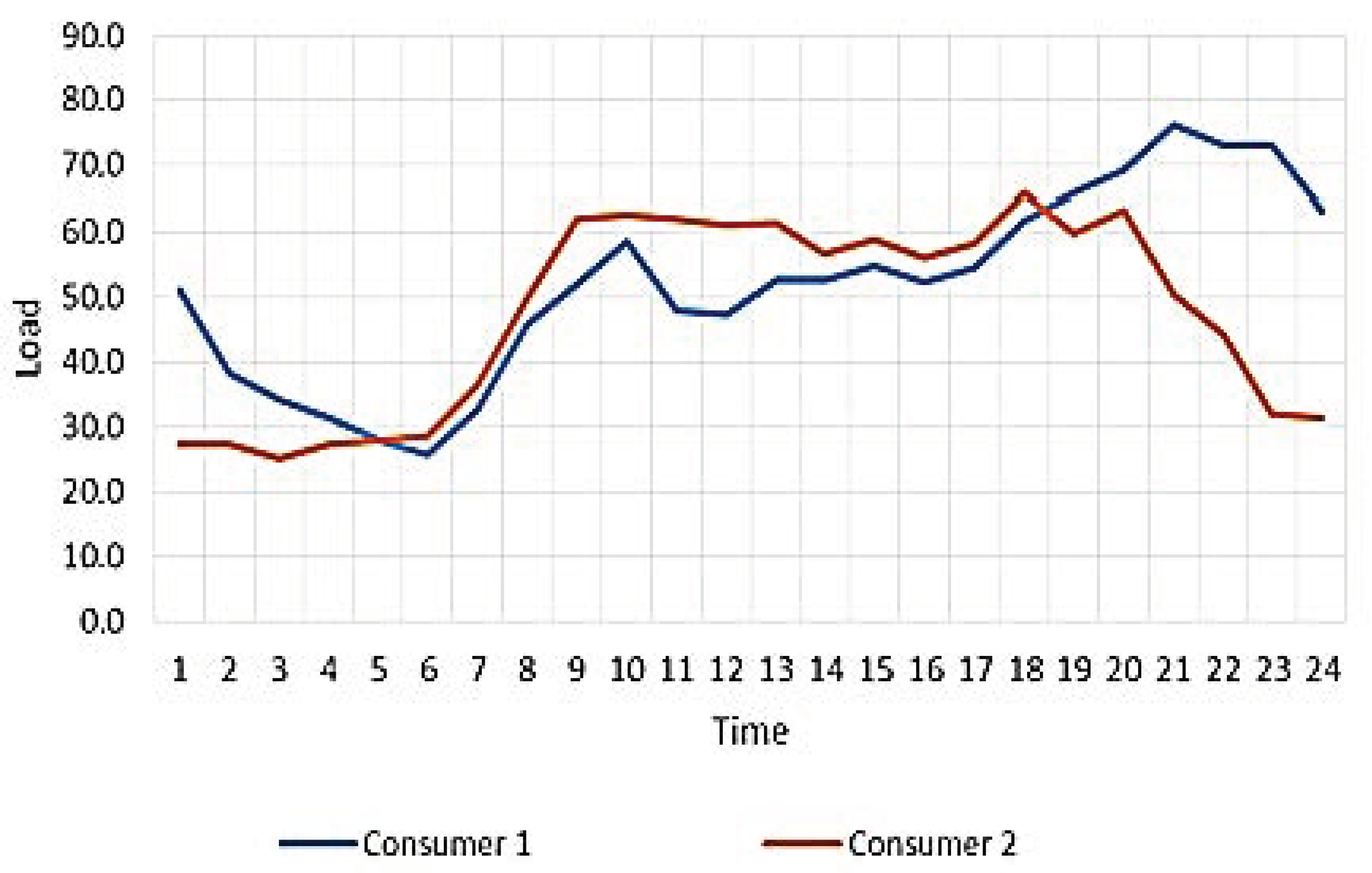
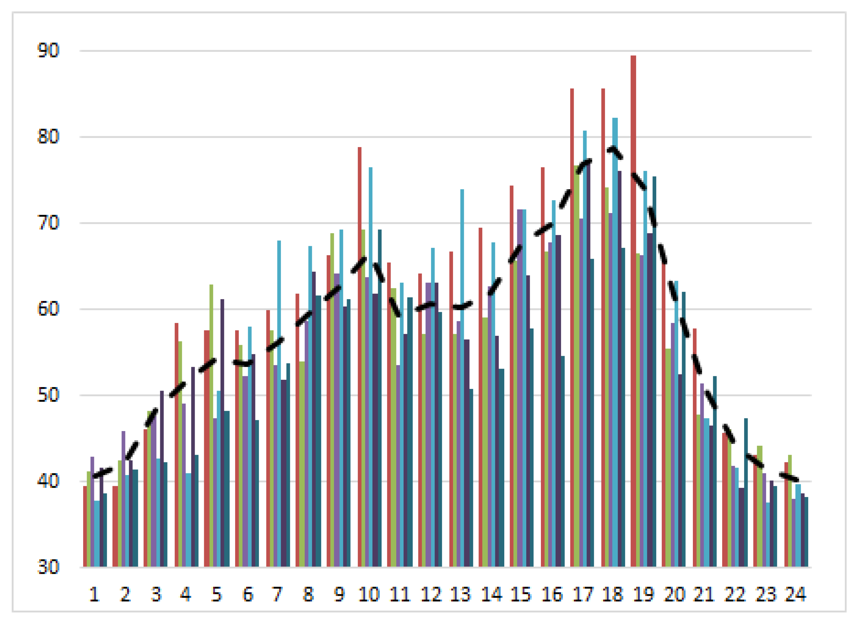
Step 1. We used the data on real loads of several consumers of different types. All consumers belong to the same category with a load below 670 kW and a low voltage level. Load curves, which are taken as a basis, represent an estimate of the mathematical expectation for the consumption per month (December 2109) for several different consumers. These loads were recorded under a Flat tariff (constant prices during the day) that was used to restore the supplier’s cost function. All prices are given in Russian rubles and correspond to Russian prices as of December 2019. For the sake of generality, we may assume that these are conventional units. Several types of consumers are analyzed:

• a dormitory with a load schedule similar to that of ordinary households (Consumer one),
• a small business that only operates during the day (Consumer 2), and
• several households with a low load (Consumer 3).

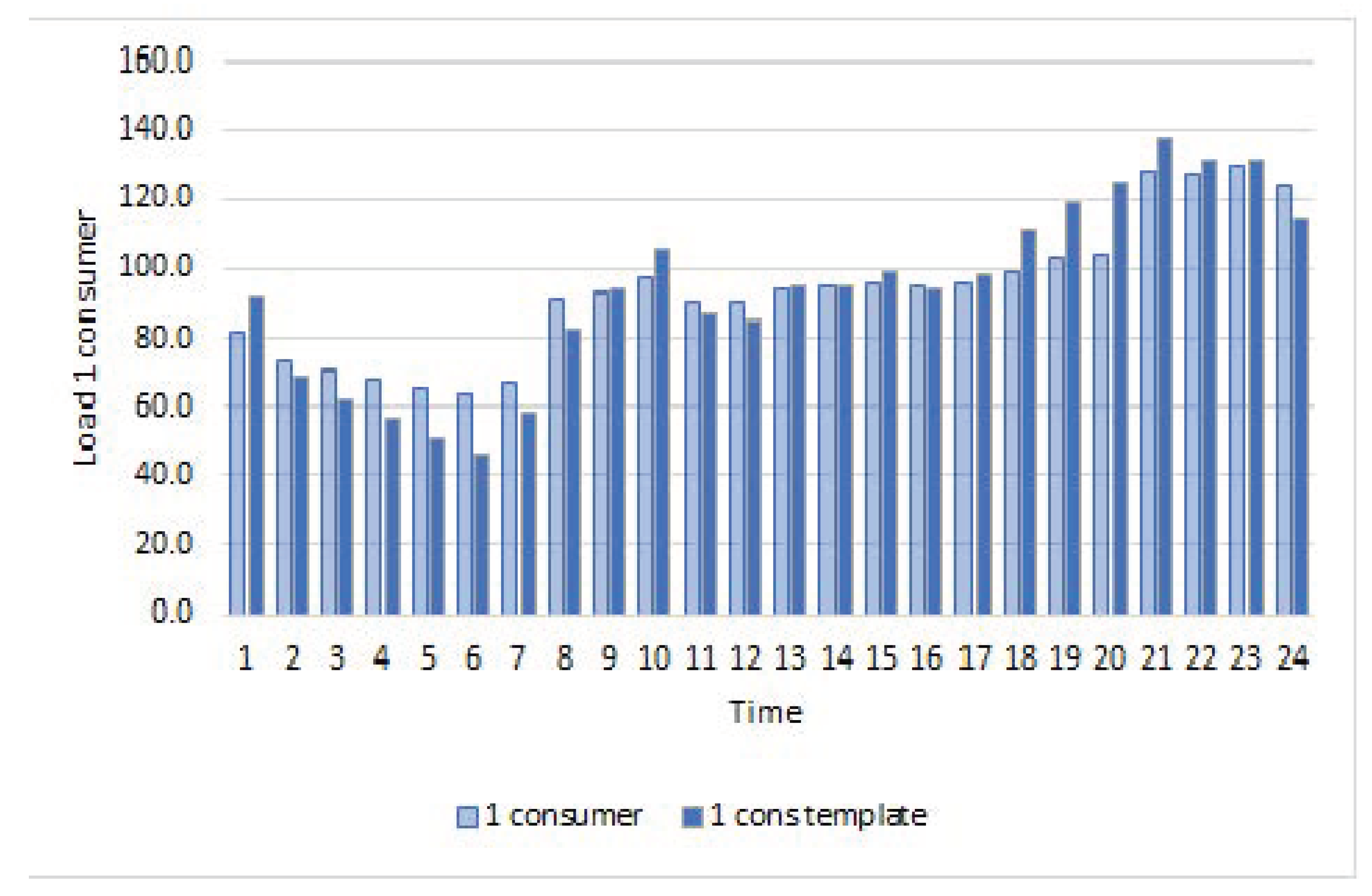
The total load changes insignificantly. The experiment will focus on redistributing the shares of different types of consumers, as well as on increasing the number of individual households within the same (approximate) total consumption. Figure 3 and Figure 4,

Table A1. Loads of two types of consumers that comprise the electric power system during the day.

t	1	3	5	7	9	11	13	15	17	19	21	23
1 Cons	51	34	28	32	52	48	53	55	54	66	76	73
2 Cons	27	25	28	36	62	62	62	59	58	60	50	32

in Appendix A show the initial average loads of Consumer 1 (${\theta }^1$) and Consumer 2 (${\theta }^2$).

The supplier’s costs are defined as quadratic $C\left(Q_t\right)\hspace{0.17em}=\hspace{0.17em}d\hspace{0.17em}·\hspace{0.17em}{Q}_t\hspace{0.17em}+\hspace{0.17em}\frac{c}{2}{Q}_t$. They have the same characteristics $d,c$ in all periods $t\hspace{0.17em}\in \hspace{0.17em}T$. If necessary, these coefficients can be varied depending on time. For the current example, $d\hspace{0.17em}=\hspace{0.17em}4,5$, $c\hspace{0.17em}=\hspace{0.17em}0.01$.

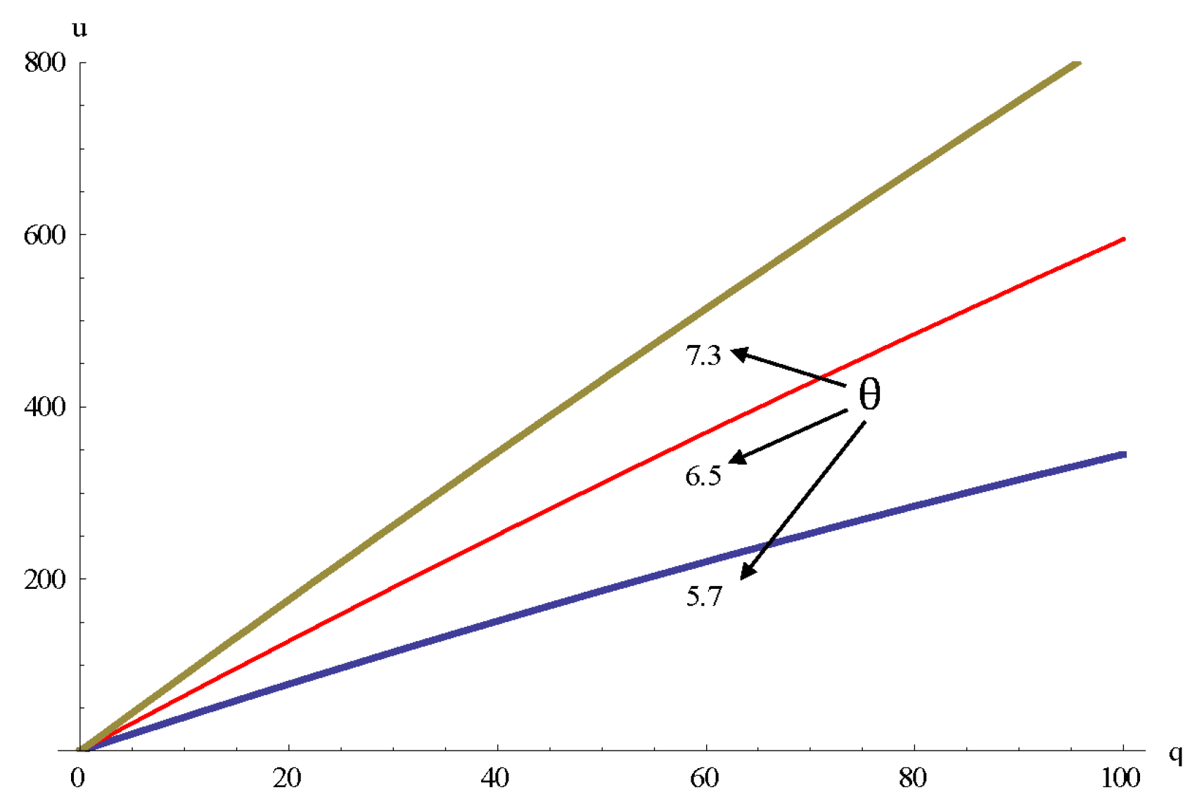
The first stage implies initialization of the consumer utility functions based on real consumption for a Flat tariff. Electricity demand is traditionally described as linear functions with low elasticity.

$$\tau \left(t,\theta \right)\hspace{0.17em}=\hspace{0.17em}{\theta }_t-\gamma \hspace{0.17em}·\hspace{0.17em}q(t,\theta ),\theta \hspace{0.17em}\in \hspace{0.17em}[\underline{\theta },\overline{\theta }],t\hspace{0.17em}\in \hspace{0.17em}T,$$

(43)

This function satisfies the properties (3)–(5): $r_u\left(z\right)\hspace{0.17em}=\hspace{0.17em}{r}_{u^{\prime }}\left(z\right)\hspace{0.17em}=\hspace{0.17em}0$. More precisely,

$$u\left(t,\hspace{0.17em}q\left(t,\hspace{0.17em}\theta \right),\hspace{0.17em}\theta \right)\hspace{0.17em}=\hspace{0.17em}\left\{\begin{array}{cc}{\theta }_t\hspace{0.17em}·\hspace{0.17em}q\left(t,\hspace{0.17em}\theta \right)\hspace{0.17em}-\hspace{0.17em}\frac{\gamma }{2}\hspace{0.17em}·\hspace{0.17em}{\left(q\left(t,\hspace{0.17em}\theta \right)\right)}^2\hfill & if0\hspace{0.17em}\le \hspace{0.17em}q\left(t,\hspace{0.17em}\theta \right)\hspace{0.17em}<\hspace{0.17em}{\theta }_t/\gamma ,\hfill \\ {\theta }_t^2/2\gamma \hfill & ifq\left(t,\hspace{0.17em}\theta \right)\hspace{0.17em}\ge \hspace{0.17em}{\theta }_t/\gamma ,\hfill \end{array}\right.t\hspace{0.17em}\in \hspace{0.17em}T.$$

(44)

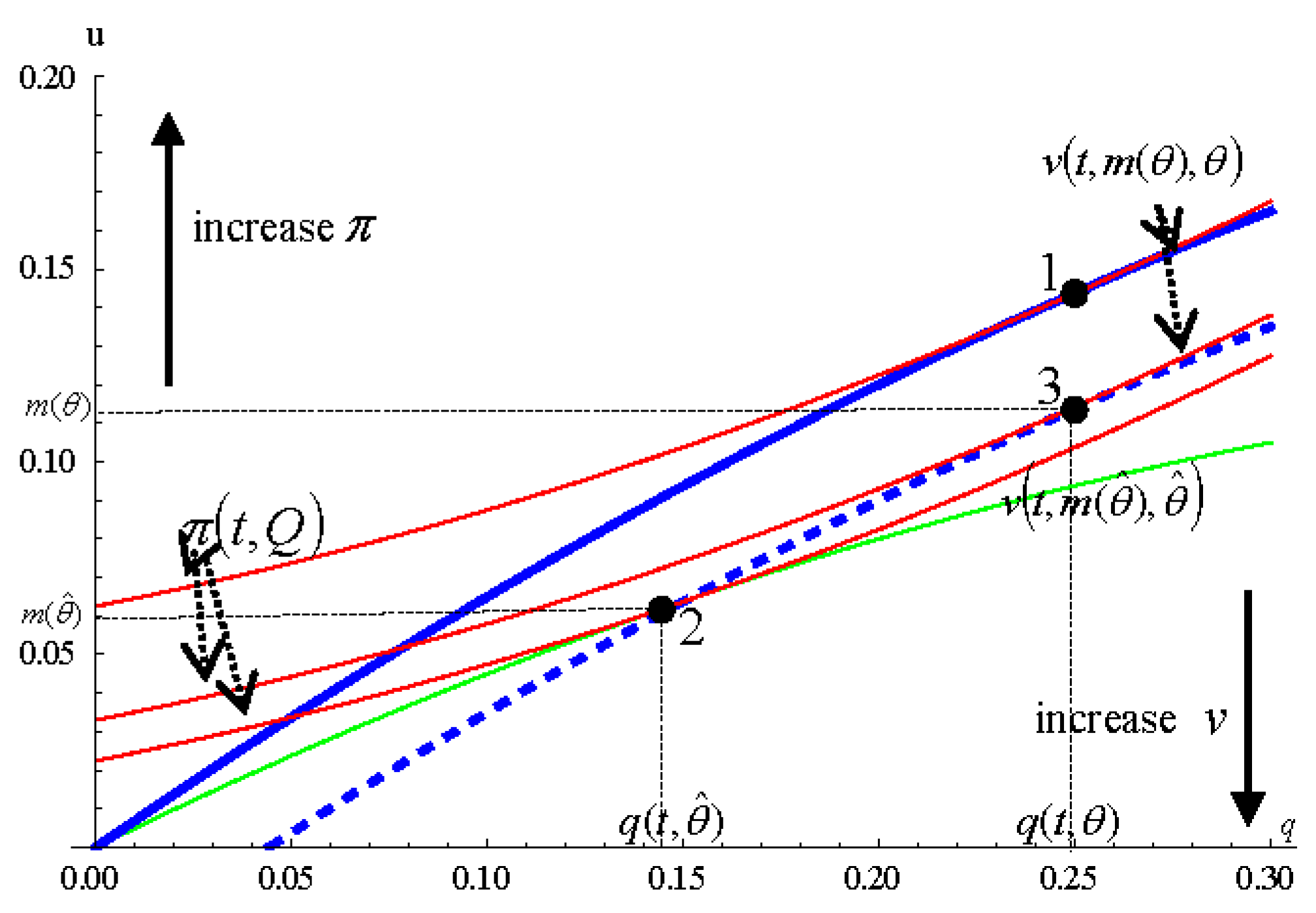
Figure 2 shows indifference curves of the utility functions for consumers of different types in a certain period of time. They satisfy the Spence–Mirrlees single crossing conditions (4) and (5). Having the initial hourly load and pricing data and assuming that the consumer $\theta$ maximizes their income $v\left(t,m\left(\theta \right),\theta \right)$ under these conditions (flat tariff, which, in this case, was $6.08$ rubles), we can restore the main characteristics of the utility function (44). For Consumers 1 and 2, $\gamma \hspace{0.17em}=\hspace{0.17em}0.011$, ${\theta }_t$, $t\hspace{0.17em}\in \hspace{0.17em}T$ vary. The results of evaluating the characteristics of utility for some periods are presented in

Table 1. The coefficient ${\theta }_t$ of the utility function (44) of Consumers 1 and 2.

t	1	3	5	7	9	11	13	15	17	19	21	23
${\theta }^1$	6.4	6.2	6.2	6.2	6.9	6.9	6.9	7.0	7.0	7.1	7.4	7.4
${\theta }^2$	6.1	6.1	6.1	6.2	7.0	7.0	7.0	6.9	6.9	6.9	6.7	6.6

. These characteristics are recalculated every time the composition of consumers changes, since the price depending on the total volume of consumption also changes.

5.2. Comparison of Different Pricing Schemes

Step 2. In this part, we will compare pricing schemes based on the Nash equilibrium principle and the maximization of social welfare (Incentive Rationality mechanism), taking into account imperfect information (optimal mechanism).

Let us solve two problems for the data presented in Section 3.1:

• finding the Nash equilibrium (38) and (39),
• social welfare maximization (41). Solving this problem corresponds to the application of the mechanism with Incentive Rationality and a solution to the problem (13)–(15).

Step 3. Based on the Incentive Rationality mechanism, we define the higher type of consumer and then form and solve (Step 4):

• problem (19)–(22) implementing the optical mechanism.

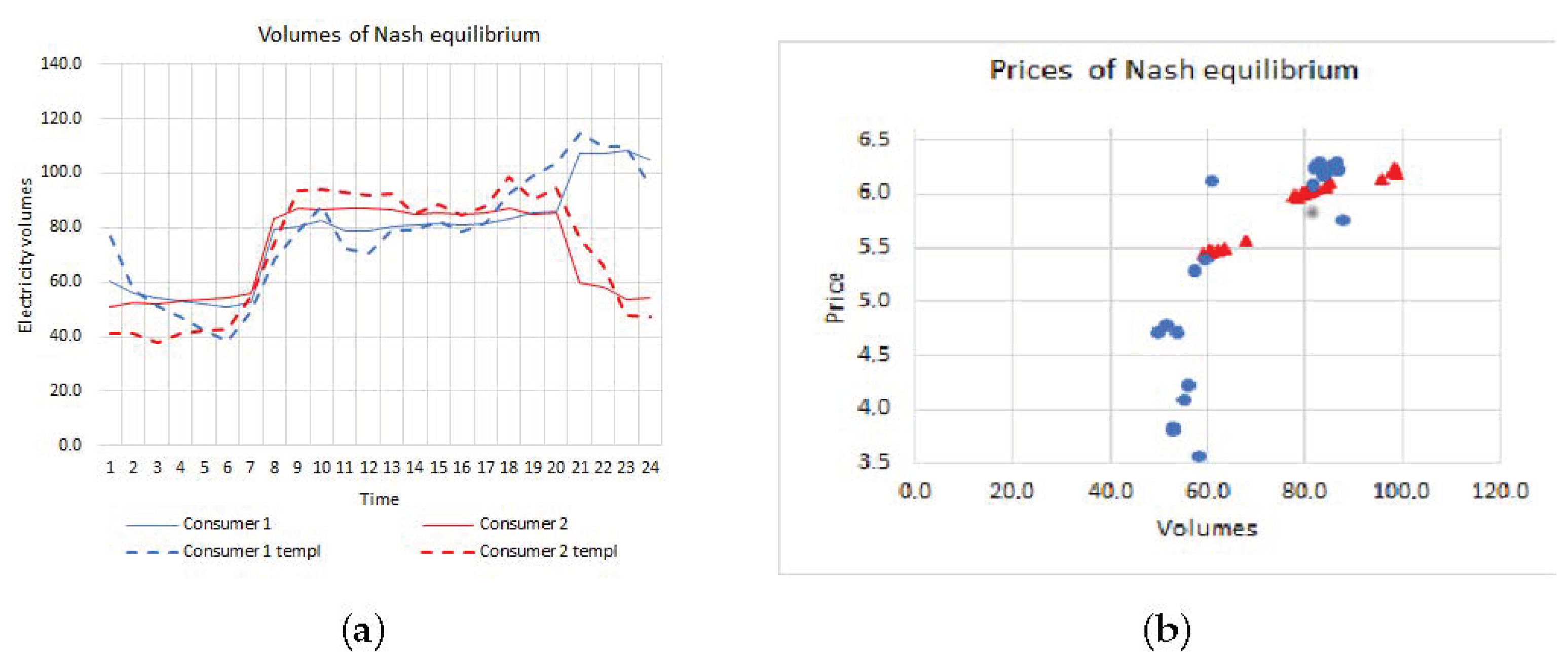
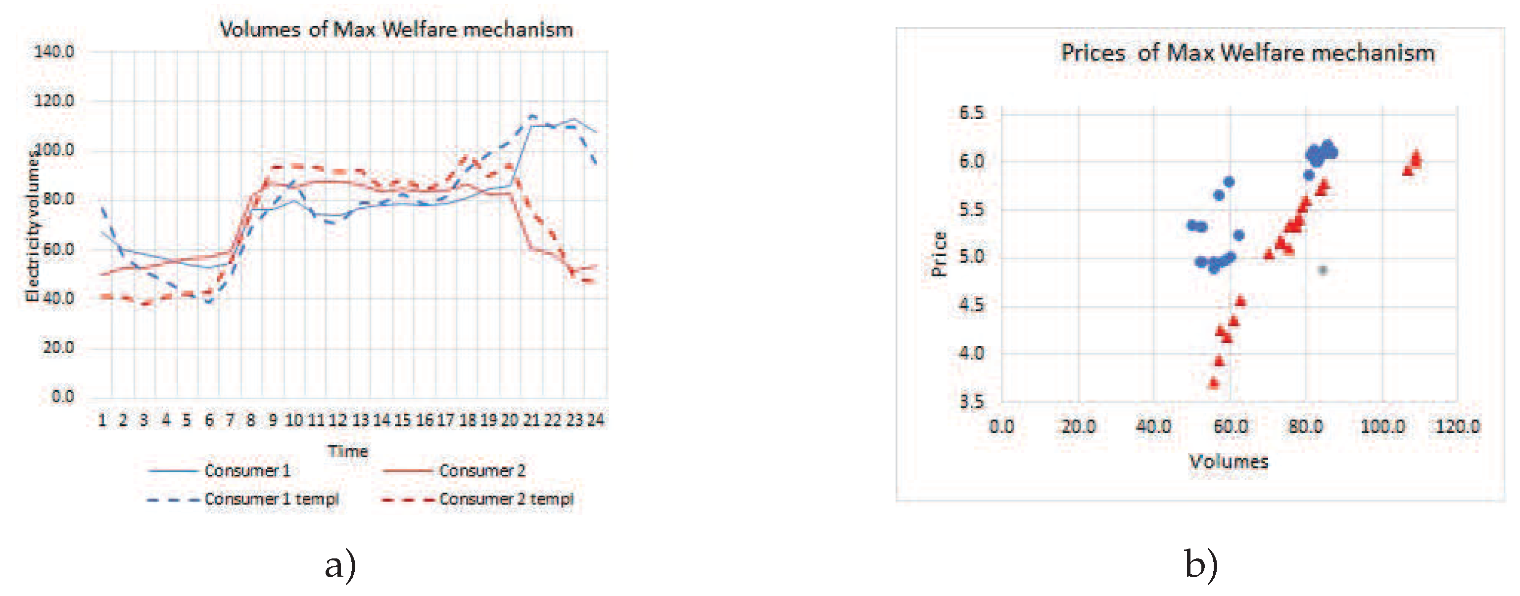
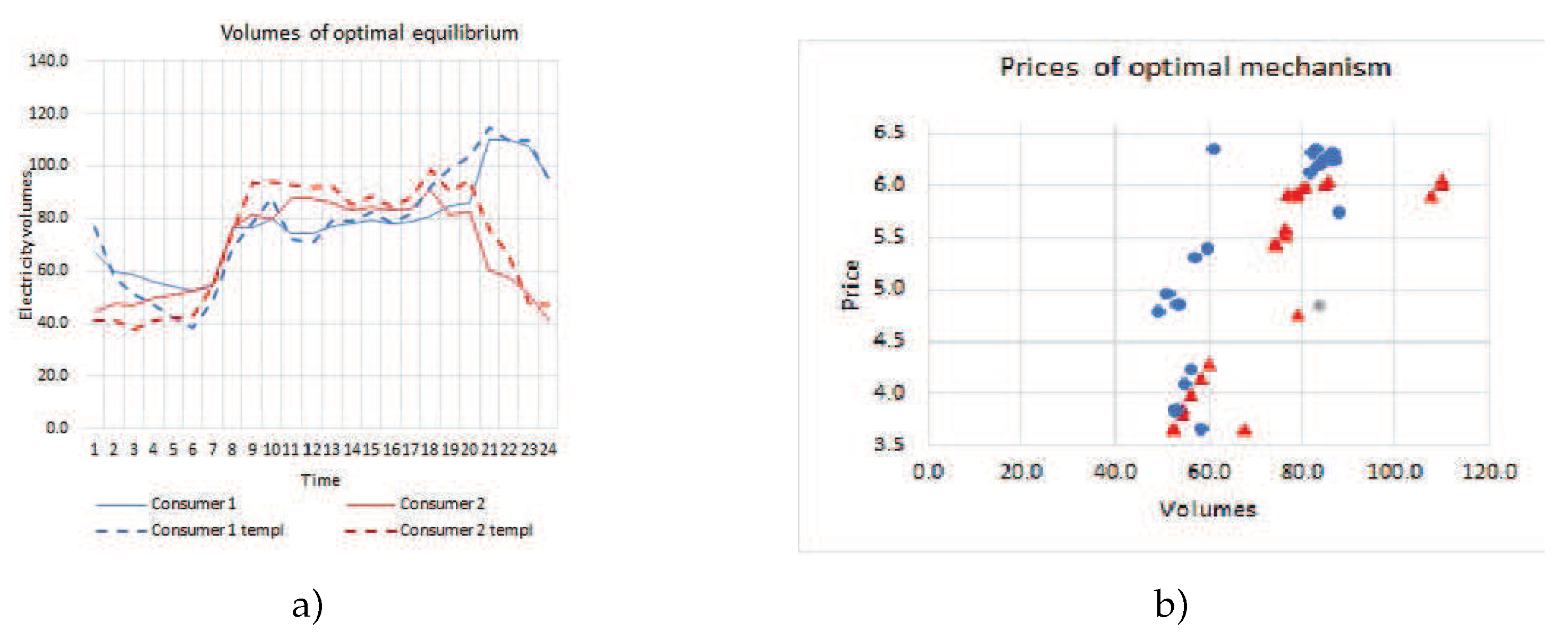
All pricing schemes that were formed as a result of solving these problems stimulate a reduction of the load during peak hours and align the schedule with respect to the average. The loads adjusted with respect to the initial state (Figure 3) are shown in Figure 5a, Figure 6a and Figure 7a, whereas the prices are given in Figure 5b, Figure 6b and Figure 7b. The general characteristics of the results obtained can be seen in

Table 2. Characteristics of equilibria with different pricing schemes, rub.

	Flat	Nash	Max Welfare	Opt Mechanism
$V\left(m\left(\theta \right),\hspace{0.17em}\theta \right)\hspace{0.17em}+\hspace{0.17em}\pi \left(m\left(\theta \right)\right)$	3732	3753	3884	3882
$\pi \left(m\left(\theta \right)\right)$	1889	2243	1981	1942
$V\left(m\left(\theta \right),\hspace{0.17em}\theta \right)$	1940	1510	1903	1942
$V^1\left(m\left({\theta }^1\right),\hspace{0.17em}{\theta }^1\right)$	1065	823	922	1067
$V^1\left(m\left({\theta }^2\right),\hspace{0.17em}{\theta }^1\right)$	-	820	1163	982
$V^2\left(m\left({\theta }^2\right),\hspace{0.17em}{\theta }^2\right)$	875	687	981	875
$V^2\left(m\left({\theta }^1\right),\hspace{0.17em}{\theta }^2\right)$	-	651	731	812
$MC\hspace{0.17em}-\hspace{0.17em}Mu\left({\theta }^1\right)$	-	2.72	0	0
$MC\hspace{0.17em}-\hspace{0.17em}Mu\left({\theta }^2\right)$	-	3.0	0	2.92

. All results are given in rubles. Profits and the consumer surplus are calculated by month. For comparison, the Table 2 in the first column shows the results for a Flat rate.

The pricing in all models is done in accordance with the incentive principle: the higher the consumption, the higher the price. This corresponds to the costs that grow with increasing consumption.

Here, $V\left(m\left(\theta \right),\hspace{0.17em}\theta \right)\hspace{0.17em}=\hspace{0.17em}{V}^1\left(m\left({\theta }^1\right),\hspace{0.17em}{\theta }^1\right)\hspace{0.17em}+\hspace{0.17em}{V}^2\left(m\left({\theta }^2\right),\hspace{0.17em}{\theta }^2\right)$, and each consumer ${\theta }^i$ chooses their contract $m\left({\theta }^i\right)$, $i\hspace{0.17em}\in \hspace{0.17em}\{1,2\}$. $V^1\left(m\left({\theta }^2\right),\hspace{0.17em}{\theta }^1\right)$ is the revenue of the consumer ${\theta }^1$ due to selecting the contract $m\left({\theta }^2\right)$ of the consumer ${\theta }^2$. The calculation results in the “Nash” and “Max Welfare” columns are carried out under the conditions of complete information, where the contract of the consumer ${\theta }^1$ is used to calculate the prices of the contract of the consumer ${\theta }^2$ only in terms of changes in the total marginal costs. After calculating the prices according to the “Nash” and “Max Welfare” rules (Table 2), the consumers are ranked in accordance with Step 2:

–

using the model of “Max Welfare”, compare the profit of the consumer ${\theta }^1$ ensured by their own contract $m\left({\theta }^1\right)$ (the profit is 922 rub.) with the profit delivered by choosing the contract of the consumer $m\left({\theta }^1\right)$ (the profit is 1163 rub.). Therefore, the strategy of the consumer ${\theta }^1$ is to choose someone else’s contract. The pricing in the “Nash” model does not give an incentive to switch to someone else’s contract, however, the consumer payoff in the “Nash” model is smaller than that in the model of “Max Welfare”;

–

similarly, consider actions of the consumer ${\theta }^2$ in the “Max Welfare” model. If ${\theta }^2$ chooses their own contract, it yields the profit of 981 rub.. However, if ${\theta }^2$ chooses the contract of ${\theta }^1$, the profit is 731 rub.. Therefore, the strategy of ${\theta }^2$ is to choose their own contract. The “Nash” model delivers the same result.

In the case considered above, the consumer ${\theta }^1$ is of higher type and has the Incentive Compatibility as an active constraint, while the consumer ${\theta }^2$ is constrained by the Incentive Rationality (20) (Step 3) (Here, we do not provide the details of ranking consumers for each of the periods $t\hspace{0.17em}\in \hspace{0.17em}T$. We carry this out when solving problems, but only give its aggregated version here.). Now, the optimization problem for creating the optimal mechanism is formulated and its solution is presented in the column “Opt mechanism”.

Analysis of the results.

1. The most effective pricing mechanism is the one that maximizes social welfare (line $V\left(m\left(\theta \right),\hspace{0.17em}\theta \right)\hspace{0.17em}+\hspace{0.17em}\pi \left(m\left(\theta \right)\right)$). Here, $V\left(m\left(\theta \right),\hspace{0.17em}\theta \right)\hspace{0.17em}=\hspace{0.17em}{V}^1\left(m\left({\theta }^1\right),\hspace{0.17em}{\theta }^1\right)\hspace{0.17em}+\hspace{0.17em}{V}^2\left(m\left({\theta }^2\right),\hspace{0.17em}{\theta }^2\right)$, and it is assumed that each consumer chooses their own contract.

2. The Nash equilibrium delivers the largest profit to the supplier. The maximum social welfare pricing reduces profits, partially redistributing the surplus of the supplier in favor of the consumers. This effect is further enhanced when prices are set according to the optimal mechanism (line $\pi \left(m\left(\theta \right)\right)$).

3. The “Nash” mechanism implements an equilibrium that is stable in terms of the incentive to choose one’s contract, since the basic principle of its formation is the Incentive Compatibility condition. On the other hand, the resulting equilibrium differs significantly from the social maximum, especially in the case of a low elasticity of demand. (As is well-known, the demand for electricity has a low elasticity, which is defined in our model through a high marginal utility. As a result, the Nash equilibrium prices appear to be higher than the marginal cost by a significant amount due to the parameter $r_u\left(t,\hspace{0.17em}\theta \right)$.) This is what makes the “Nash” pricing model faulty.

4. The “Max Welfare” pricing model is not feasible in practice. The contracts it designs do not satisfy all consumers. Only the low type will choose their contract. It will be beneficial for a higher type to adhere to the contract of another consumer.

5. The optimal mechanism “Opt Mechanism” forms stable contracts in the sense that the consumer chooses “their own” contract. Table 2 shows that the profit ensured by choosing their own contract (truthfully declaring their own type) is higher than when choosing someone else’s contract (for ${\theta }^1$ $V^1\left(m\left({\theta }^1\right),\hspace{0.17em}{\theta }^1\right)\hspace{0.17em}=\hspace{0.17em}1067\hspace{0.17em}\ge \hspace{0.17em}$ $V^1\left(m\left({\theta }^2\right),\hspace{0.17em}{\theta }^1\right)\hspace{0.17em}=\hspace{0.17em}982$ and similarly for ${\theta }^2$).

6. Due to the asymmetry of information in the optimal mechanism, social welfare is partially lost in comparison with the “Max Welfare”. Pricing is efficiently done for the higher type consumers, and the lower type loses some of their profit in their favor. This is clearly seen from the last two rows of Table 2. Here, we have the indicators of the mismatch between marginal costs and marginal utilities. For “Max Welfare”, the marginal utility $Mu\left({\theta }^i\right)\hspace{0.17em}=\hspace{0.17em}{\sum }_{t\in T}{u}^{\prime }\left(t,\hspace{0.17em}q\left(t,\hspace{0.17em}{\theta }^i\right),{\theta }^i\right)$ is equal to the marginal cost $MC\hspace{0.17em}=\hspace{0.17em}{\sum }_{t\in T}{C}^{\prime }\left(Q_t\right)$. This does not happen in the optimal mechanism.

7. The optimal mechanism is as close as possible to the solution that delivers the maximum social welfare.

5.3. Features of Optimal Contracts for Various Configurations of the Electric Power Systems

This part discusses several examples of different consumer compositions. In the first paragraph, there are two consumers, but of different sizes. This is different from the previous example, where the total load was approximately equal throughout the day. The second case considers three consumers, each assigned to their contract. The third case focuses on the situation with many small consumers.

5.3.1. Two Consumers of Different Sizes

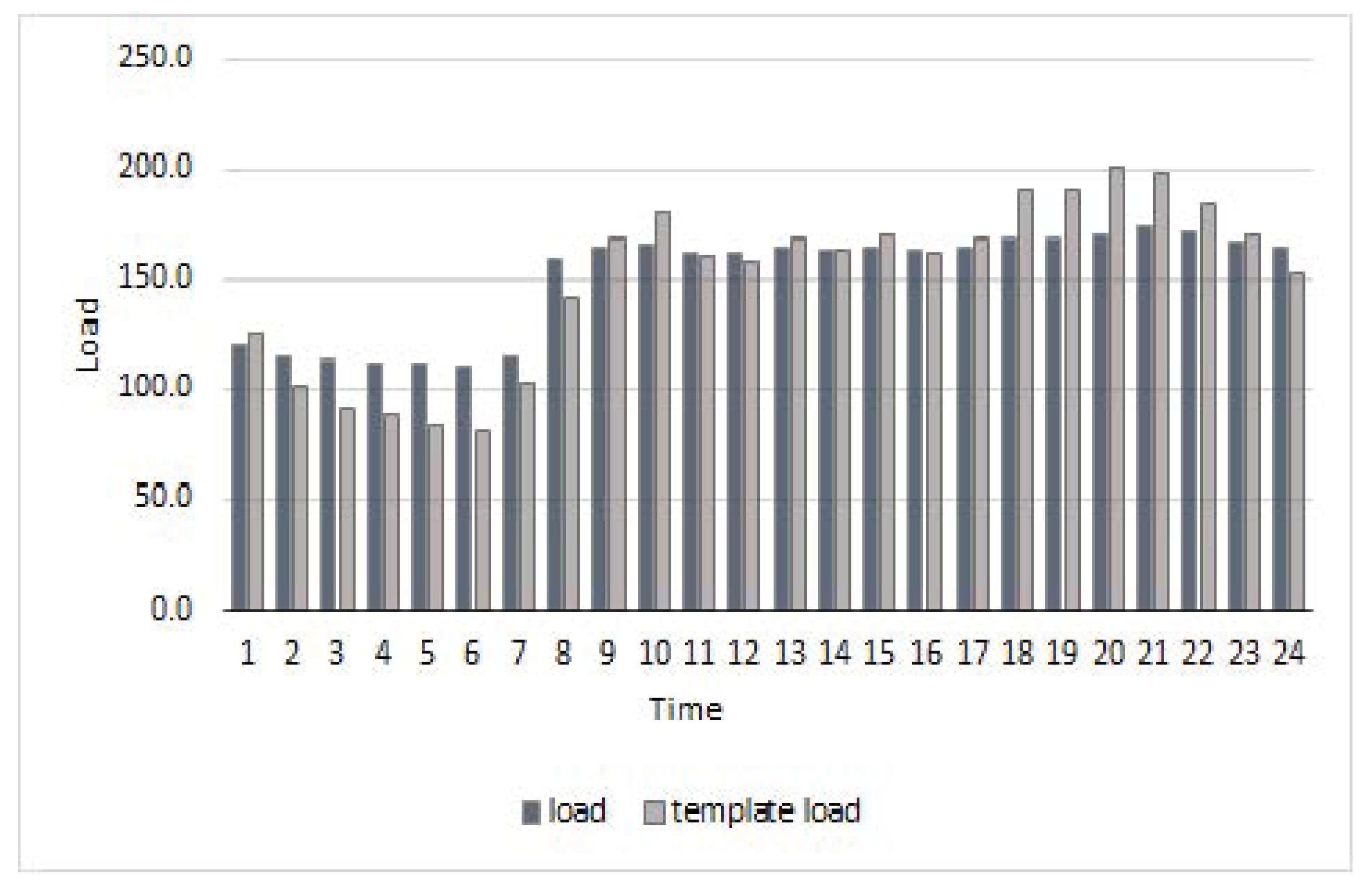
We consider consumers with the same load configurations as before. The difference is that Consumer 1 is now larger and accounts for about 60% of the aggregated load, and Consumer 2 is, respectively, smaller. Figure 8 shows the load graphs optimized by the optimal mechanism. Figure 9 demonstrates the effect that such pricing has on the system as a whole. It also shows the aggregated load before and after applying incentive pricing. For the given example, the scatter was calculated with respect to the day average. The use of incentive prices for several consumers at the same time can reduce the the scatter around the average up to 32% for the given conditions.

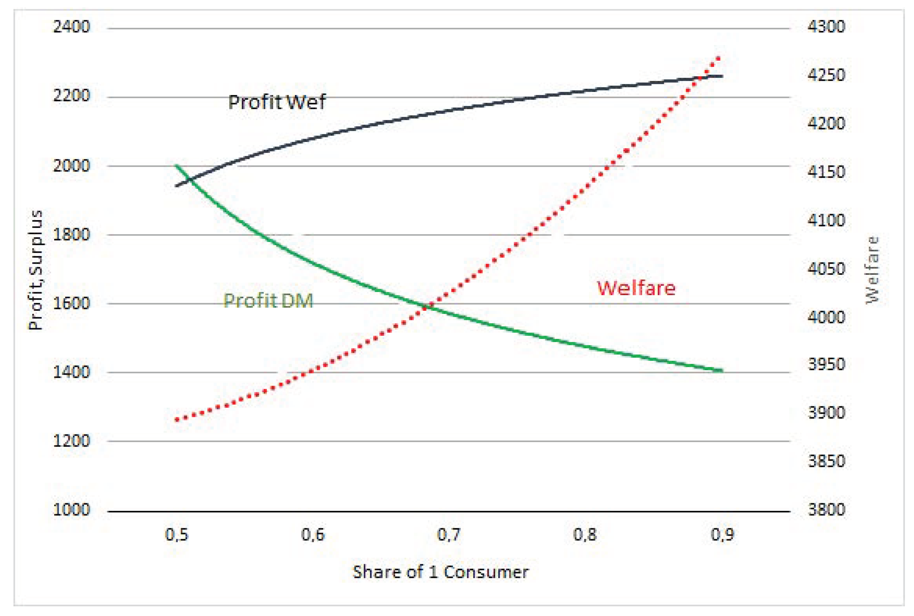
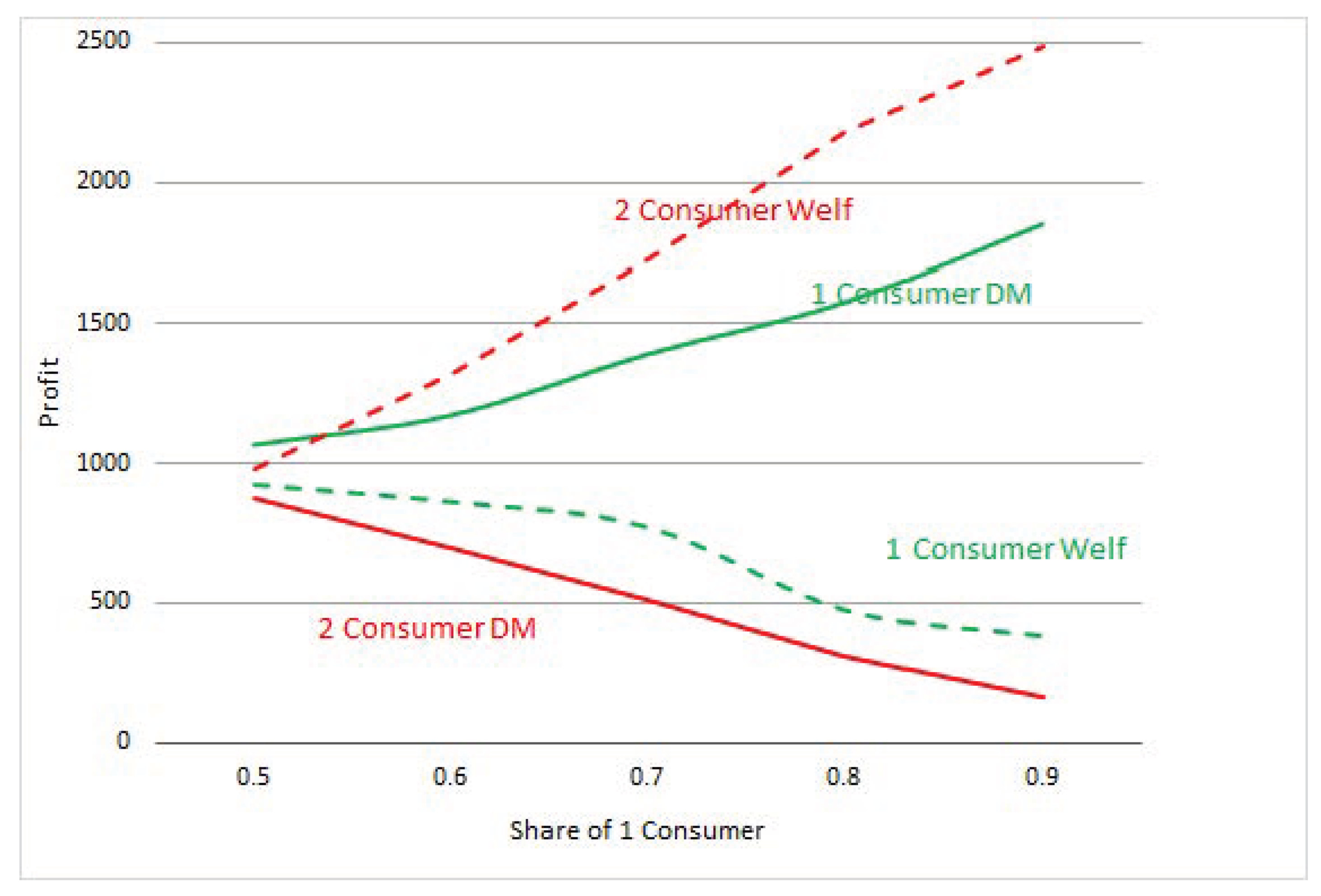
Next, we present the results of numerical modeling of the equilibrium parameters when Consumer 1 (higher type) shifts from 0.5 to 0.9. Figure 10 and Figure 11 show the changes in the supplier’s profit, social welfare, consumer surplus for Consumers 1 and 2. A complete table of values is given in Appendix A 

Table A2. Loads of three types of consumers that comprise the electric power system during the day.

Time	Consumer	1	3	5	7	9	11	13	15	17	19	21	23
Load	1	50.8	44.3	41.5	42.1	63.0	62.6	65.3	66.7	64.4	76.7	82.2	84.3
	2	28.1	31.8	34.6	36.9	58.6	60.8	60.3	58.7	56.4	51.9	45.2	39.4
	3	31.5	29.0	27.6	27.2	42.4	38.1	36.1	36.5	43.3	52.5	55.1	54.2
Prices	1	5.25	5.10	5.49	5.52	5.87	6.08	6.10	5.98	6.02	5.39	6.24	6.41
	2	4.89	4.92	5.49	5.52	5.85	6.08	6.10	5.97	6.01	4.91	6.39	6.37
	3	4.97	4.85	5.46	5.49	6.12	6.04	6.03	6.03	6.13	4.92	6.37	6.32

.

The optimal mechanism creates a separating equilibrium with incentives to reduce the load. With an increase in the share of higher-type consumers in the power system, the following occurs:

1. Redistribution of social wealth (Figure 10 and Figure 11);

2. The supplier’s profit falls (Figure 10, green line);

3. Growth of the overall welfare (Figure 10, red line);

4. Consumer surplus among higher-type consumers grows (Figure 11, green solid line) partly due to a decrease in consumer surplus of lower-type consumers (Figure 11, red solid line) and partly due to the supplier’s profits.

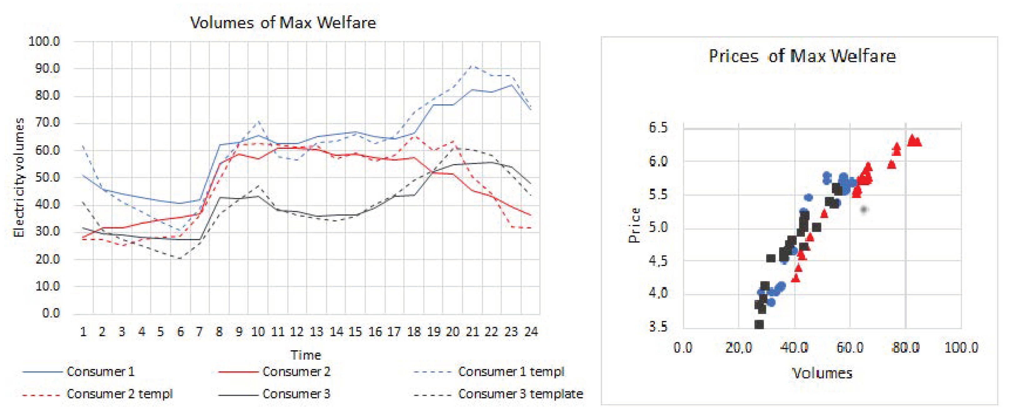
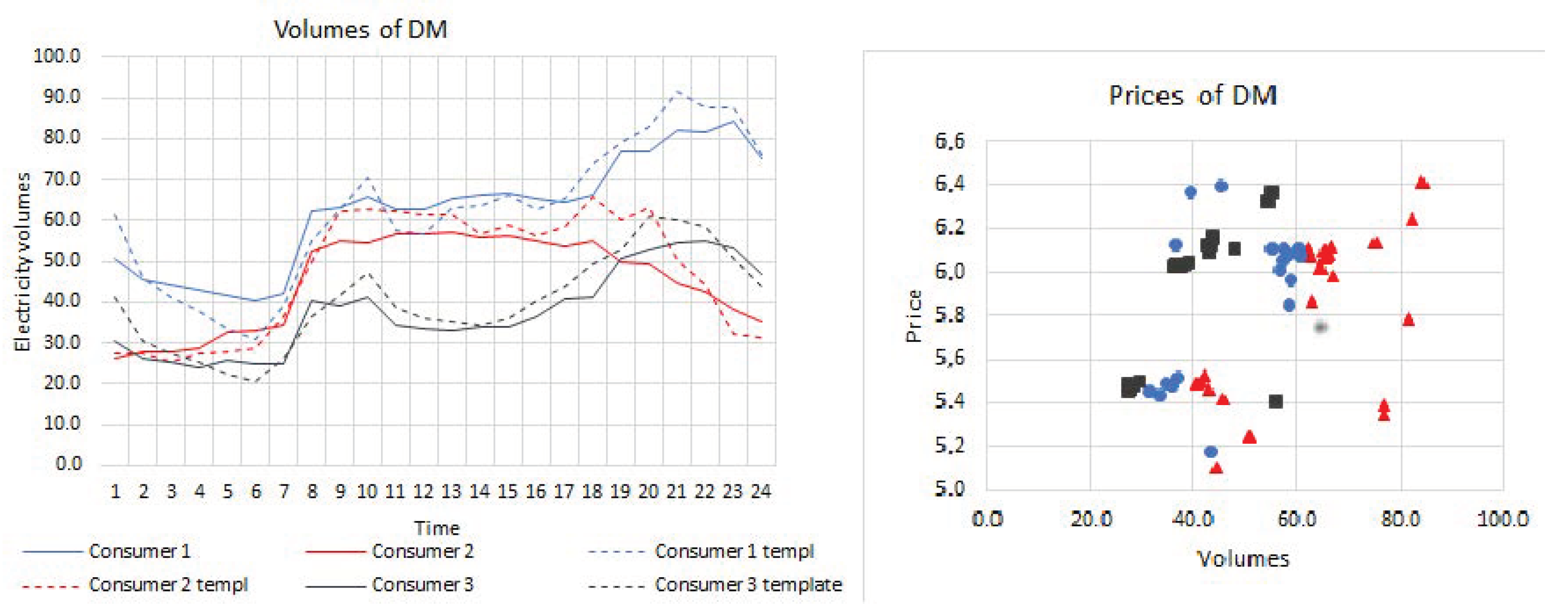
5.3.2. Assigning Contracts to Three Different Consumers of the Power System

We considered a system that has three consumers of different supply. The graph of Consumer 3 represents a typical household load. Using the algorithm given in Section 2.2, we determined the optimal loads and prices for each of the consumers. Figure 12 and Figure 13 show the main characteristics of the equilibrium obtained by the two models in comparison with the initial Flat tariff.

Table 3. Equilibrium characteristics for three consumers as calculated with the optimal mechanism.

Opt Mechanism		Surplus	1 Consumer	2 Consumer	3 Consumer
Wefrare	3561	Price 1	755.2	552.3	213.5
Profit	1941	Price 2	730.2	612.0	73.9
Surplus Cons	1620	Price 3	688.3	554.5	252.8

summarizes the general equilibrium characteristics for the optimal mechanism. Price 1 denotes the prices offered to Consumer 1. It can be seen that consumers choose their own prices as the consumer surplus is maximal. For comparison,

Table 4. Characteristics of the maximum welfare solution for three consumers.

Opt Mechanism		Surplus	1 Consumer	2 Consumer	3 Consumer
Wefrare	3562	Price 1	1045.0	842.1	824.3
Profit	141	Price 2	1341.1	1222.8	363.7
Surplus Cons	3420	Price 3	1588.1	1454.3	1152.6

shows the results of calculations according to the welfare maximum model, where we have a mixing equilibrium, since it is profitable for Consumers 1 and 2 to switch to the contract of Consumer 3. In addition, if the prices of Consumer 3 are unavailable, Consumer 1 chooses the contract of Consumer 2.

By reacting to prices, electricity users regulate their load. For the given conditions, price-dependent optimization of the load by consumers decreases the variation in the electricity consumption with respect to the daily average by 16%. This is less than for two consumers, and is associated with the characteristics of the load of individual users.

The examples given above demonstrated the effectiveness of the proposed mechanism with two or three types of consumers. If we introduce more prices in the market, this will cause confusion for consumers and, therefore, such a situation is not considered here. At the same time, if the promising pricing schemes embedded in smart grid systems target individual consumers, then the proposed approach may also be relevant.

In our study, testing was carried out with a large number of users and two pricing schemes. We considered from 10 to 60 consumers that were divided into two types. We obtained regularities similar to Section 5.3.1. The higher the type of consumers, the larger the supplier’s profit and the consumer surplus. The proposed optimal mechanism also proved to be effective, confirming possible scaling to any number of participants.

6. Conclusions

Electricity markets are actively regulated by the state as power supply systems are critical infrastructures for the economy and life. Therefore, price regulation methods are aimed at maximizing social welfare. This paper discusses the pricing method driven by welfare maximization models and reveals its inconsistency. We demonstrated that, in this case, there was a mixed equilibrium where all consumers tended to choose the same prices. As a result, the maximum social welfare was not achieved and the incentives to optimize the consumer’s load were reduced.

We propose an optimal mechanism based on the fulfillment of the Incentive Rationality and Incentive Compatibility conditions. We used this mechanism to set prices, and, as a result, we obtained a separating equilibrium, when each consumer was inclined to choose their own prices. The solution obtained was close to the maximum welfare. This also enabled optimization of the load schedule of the electric power system, which leads to more effective functioning (the scatter is reduced with respect to the daily average, and pronounced peaks are smoothed out). This is what constitutes the novelty and relevance of our study, which is in contrast to the available publications that propose to determine tariffs in accordance with the Nash equilibrium, as a result of which, a significant part of the social welfare is lost.

To formalize the model, a number of statements were proven. One of the key statements is the proposition that it is possible to use the Incentive Compatibility condition in certain periods to build a pricing mechanism for several periods. This will ensure the fulfillment of the Incentive Compatibility condition, which is crucial for the optimal mechanism during the entire time interval considered. The proposed mechanism will also work in a situation where, in one period of time, the first consumer receives a utility from a unit of electricity that is higher than the second consumer, and, in another period, they change roles. Then, the consumer types are not transitive with respect to each other over time.

The mechanism was demonstrated on various configurations of a multi-consumer power system. We compared pricing schemes according to the Nash, the maximum social welfare, and our mechanism. We demonstrated the effectiveness of the “Opt Mechanism” when compared to other schemes.

The use of smart meters enables the regulation of prices and consumption on the go. Electricity supply companies can use the proposed pricing mechanism in real-life problems. The mechanism is quite straightforward for implementation. and it will work successfully when planning for a day that is a week in advance, through providing incentives for the consumer to correctly disclose their types and optimize the load, which will ensure the effectiveness of the pricing scheme for the entire power system.

To develop the current task, we propose to study the issues of dividing a large number of consumers into several consistent groups for the optimal formation of the load schedule. In this study, this issue was resolved for individual consumers; the transition to a group is associated with additional difficulties in the formation of an aggregated utility function that will not violate the incentives for individual players to be in it.

References

1. Kirschen, D.S. Demand-side view of electricity markets. IEEE Trans. Power Syst. 2003, 18, 520–527. [Google Scholar] [CrossRef] [Green Version]
2. Tirole, J.; Jean, T. The Theory of Industrial Organization; MIT Press: Cambridge, MA, USA, 1993. [Google Scholar]
3. Vogelsang, I.; Finsinger, J. A regulatory adjustment process for optimal pricing by multiproduct monopoly firms. Bell J. Econ. 1979, 10, 157–171. [Google Scholar] [CrossRef]
4. Borenstein, S.; Jaske, M.; Rosenfeld, A. Dynamic Pricing, Advanced Metering, and Demand Response in Electricity Markets; Center for the Study of Energy Markets; University of California: Oakland, CA, USA, 2002. [Google Scholar]
5. Meyabadi, A.F.; Deihimi, M.H. A review of demand-side management: Reconsidering theoretical framework. Renew. Sustain. Energy Rev. 2017, 80, 367–379. [Google Scholar] [CrossRef]
6. Alasseri, R.; Tripathi, A.; Rao, T.J.; Sreekanth, K.J. A review on implementation strategies for demand side management (DSM) in Kuwait through incentive-based demand response programs. Renew. Sustain. Energy Rev. 2017, 77, 617–635. [Google Scholar] [CrossRef]
7. Breukers, S.C.; Heiskanen, E.; Brohmann, B.; Mourik, R.M.; Feenstra, C.F. Connecting research to practice to improve energy demand-side management (DSM). Energy 2011, 36, 2176–2185. [Google Scholar] [CrossRef] [Green Version]
8. Niromandfam, A.; Yazdankhah, A.S.; Kazemzadeh, R. Designing risk hedging mechanism based on the utility function to help customers manage electricity price risks. Electr. Power Syst. Res. 2020, 185, 106365. [Google Scholar] [CrossRef]
9. Abapour, S.; Nazari-Heris, M.; Mohammadi-Ivatloo, B.; Hagh, M.T. Game theory approaches for the solution of power system problems: A comprehensive review. Arch. Comput. Methods Eng. 2020, 27, 81–103. [Google Scholar] [CrossRef]
10. Mohsenian-Rad, A.H.; Wong, V.W.; Jatskevich, J.; Schober, R.; Leon-Garcia, A. Autonomous demand-side management based on game-theoretic energy consumption scheduling for the future smart grid. IEEE Trans. Smart Grid 2010, 1, 320–331. [Google Scholar] [CrossRef] [Green Version]
11. Samadi, P.; Mohsenian-Rad, H.; Schober, R.; Wong, V.W. Advanced demand side management for the future smart grid using mechanism design. IEEE Trans. Smart Grid 2012, 3, 1170–1180. [Google Scholar] [CrossRef]
12. Fadlullah, Z.M.; Quan, D.M.; Kato, N.; Stojmenovic, I. GTES: An optimized game-theoretic demand-side management scheme for Smart Grid. IEEE Syst. J. 2014, 8, 588–597. [Google Scholar] [CrossRef]
13. Aizenberg, N.; Voropai, N. The Interaction of Consumers and Load Serving Entity to Manage Electricity Consumption. In Communications in Computer and Information Science; Springer: Cham, Switzerland, 2019; Volume 1090, pp. 147–162. [Google Scholar]
14. Aizenberg, N.; Stashkevich, E.; Voropai, N. Forming rate options for various types of consumers in the retail electricity market by solving the adverse selection problem. Int. Public Adm. 2019, 42, 1349–1362. [Google Scholar] [CrossRef]
15. Muthirayan, D.; Kalathil, D.; Poolla, K.; Varaiya, P. Mechanism design for demand response programs. IEEE Trans. Smart Grid 2019, 11, 61–73. [Google Scholar] [CrossRef] [Green Version]
16. Tsaousoglou, G.; Steriotis, K.; Efthymiopoulos, N.; Smpoukis, K.; Varvarigos, E. Near-optimal demand side management for retail electricity markets with strategic users and coupling constraints. Sustain. Energy Grids Netw. 2019, 19, 100236. [Google Scholar] [CrossRef]
17. Hartway, R.; Price, S.; Woo, C.K. Smart meter, customer choice and profitable time-of-use rate option. Energy 2014, 24, 895–903. [Google Scholar] [CrossRef]
18. Aizenberg, N.; Stashkevich, E. Game-theoretic Approach to Electricity Retail Pricing Design for Demand Response Management in Russian Regions. In E3S Web of Conferences; EDP Sciences: Les Ulis, France, 2020; Volume 209, p. 03001. [Google Scholar]
19. Qiu, Y.; Colson, G.; Wetzstein, M.E. Risk preference and adverse selection for participation in time-of-use electricity pricing programs. Resour. Energy Econ. 2017, 47, 126–142. [Google Scholar] [CrossRef] [Green Version]
20. Alasseur, C.; Ekeland, I.; Elie, R.; Hernandez Santibanez, N.; Possamai, D. An adverse selection approach to power pricing. SIAM J. Control Optim. 2020, 58, 686–713. [Google Scholar] [CrossRef]
21. Chen, Y.; Wei, W.; Liu, F.; Shafie-khah, M.; Mei, S.; Catalao, J.P. Optimal contracts of energy mix in a retail market under asymmetric information. Energy 2018, 165, 634–650. [Google Scholar] [CrossRef]
22. Yang, P.; Tang, G.; Nehorai, A. A game-theoretic approach for optimal time-of-use electricity pricing. IEEE Trans. Power Syst. 2012, 28, 884–892. [Google Scholar] [CrossRef]
23. Mas-Colell, A.; Whinston, M.D.; Green, J.R. Microeconomic Theory; Oxford University Press: New York, NY, USA, 1995; Volume 2, pp. 857–917. [Google Scholar]
24. Maskin, E.; Riley, J. Monopoly with incomplete information. RAND J. Econ. 1984, 15, 171–196. [Google Scholar] [CrossRef]
25. Cremer, J.; McLean, R.P. Full extraction of the surplus in Bayesian and dominant strategy auctions. Econom. J. Econom. Soc. 1988, 56, 1247–1257. [Google Scholar] [CrossRef]
26. Albert, M.; Conitzer, V.; Stone, P. Automated design of robust mechanisCrémer. In Proceedings of the AAAI Conference on Artificial Intelligence, San Francisco, CA, USA, 4–9 February 2017; Volume 31, pp. 298–304. [Google Scholar]
27. Weber, T.A. Optimal Control Theory with Applications in Economics; MIT Press: Cambridge, MA, USA, 2011; pp. 183–202. [Google Scholar]
28. Spulber, D.F. Monopoly Pricing of Capacity Usage Under Asymmetric Information. J. Ind. Econ. 1993, 41, 241–257. [Google Scholar] [CrossRef]
29. Rosen, J.B. Existence and uniqueness of equilibrium points for concave n-person games. Econometrica 1965, 33, 347–351. [Google Scholar] [CrossRef] [Green Version]
30. Myerson, R. Bayesian Equilibrium and Incentive-Compatibility: An Introduction. In Social Goals and Social Organization; Hurwicz, L., Schmeidler, D., Sonnenschein, H., Eds.; Cambridge University Press: New York, NY, USA, 1985. [Google Scholar]
31. Jackson, M.O. Mechanism theory. In The Encyclopedia of Life Support Systems; Derigs, U., Ed.; EOLSS Publishers: Oxford UK, 2003. [Google Scholar]
Figure 1. The formation of mixing and separating equilibria. Indifference curves of utility functions for a higher type consumer θ are shown in blue, and for a lower type consumer θ ^ in green. Indifference curves of the supplier’s profit are shown in red.
Mathematics 09 01147 g001
Figure 2. Utility function with θ .
Mathematics 09 01147 g002
Figure 3. The loads of Consumers 1 and 2.
Mathematics 09 01147 g003
Figure 4. the load of Consumer 1 in a few days.
Mathematics 09 01147 g004
Figure 5. The Nash equilibrium pricing. The (a) optimal load and (b) prices.
Mathematics 09 01147 g005
Figure 6. The maximum welfare pricing. The optimal load (a) and prices (b).
Mathematics 09 01147 g006
Figure 7. The optimal mechanism pricing. The optimal load (a) and prices (b).
Mathematics 09 01147 g007
Figure 8. Load of Consumer 1 when its share when the share is 0.6 of the aggregated load.
Mathematics 09 01147 g008
Figure 9. The aggregated load of the system load of the system before applying the optimal mechanism and after.
Mathematics 09 01147 g009
Figure 10. Load of Consumer 1 when its share when its share is 0.6 of the aggregated load.
Mathematics 09 01147 g010
Figure 11. Load of Consumer 1 when its share when its share is 0.6 of the aggregated load.
Mathematics 09 01147 g011
Figure 12. Chart of the load and prices before and after applying maximizing welfare pricing (“Max Welfare”).
Mathematics 09 01147 g012
Figure 13. Chart of the load and prices before and after applying the optimal mechanism (“Opt mechanism”).
Mathematics 09 01147 g013