On the Existence and Uniqueness of the ODE Solution and Its Approximation Using the Means Averaging Approach for the Class of Power Electronic Converters

Abstract

Power electronic converters are mathematically represented by a system of ordinary differential equations discontinuous right-hand side that does not verify the conditions of the Cauchy-Lipschitz Theorem. More generally, for the properties that characterize their discontinuous behavior, they represent a particular class of systems on which little has been investigated over the years. The purpose of the paper is to prove the existence of at least one global solution in Filippov’s sense to the Cauchy problem related to the mathematical model of a power converter and also to calculate the error in norm between this solution and the integral of its averaged approximation. The main results are the proof of this theorem and the analytical formulation that provides to calculate the cited error. The demonstration starts by a proof of local existence provided by Filippov himself and already present in the literature for a particular class of systems and this demonstration is generalized to the class of electronic power converters, exploiting the non-chattering property of this class of systems. The obtained results are extremely useful for estimating the accuracy of the averaged model used for analysis or control of the effective system. In the paper, the goodness of the analytical proof is supported by experimental tests carried out on a converter prototype representing the class of power electronics converter.

1. Introduction

The Ordinary Differential Equations (ODEs) with discontinuous right-hand side are one of the common frontiers between Mathematics and Engineering. Several phenomena in mechanical, control systems and particularly in power electronics are the main sources of motivation of this study. Power electronics is an area of electrical engineering in enormous expansions; it studies and develops many circuit configurations used for the conversion of energy from electrical to electrical [1]. The aim is to modify the energy parameters, for example, converting a constant voltage of 4000 V available on a catenary of a railway into a sinusoidal voltage on a train or converting the sinusoidal voltage available in our houses in constant voltage to charge the batteries of our smartphones or to supply domestic devices. The apparatuses that realize this conversion (called “power electronic Converters”) can convert in general all the forms of electrical energy (alternating, continuous, periodic) into a form of electrical energy with desired and adjustable voltage and frequency values. These converters are widely used in every industrial field, in transport, in home automation and in electricity distribution systems. The converters are made by serial and/or parallel connection of various power semiconductor components, called “switches”, because they are used exactly as switches, i.e., only in “ON” or “OFF” state. Caused by this periodic switching action, the differential equations representing the power electronic converters are characterized by a sudden change. In other words, they are generally described by nonlinear ODE’s system (switched model) discontinuous right-hand side, (i.e., depending on a T-periodic function with “time discontinuity” and “state discontinuity”) under periodic forcing, and then the existence and the uniqueness of the solution cannot be found with usual methods. It is known that the averaging method is a powerful technique used for the analysis of the nonlinear differential systems. They have a long history starting by the works of Lagrange and successively by the works of Jacobi and Poincaré regarding the perturbation theory. The first results regarding the feasibility of the averaging approach were fixed by Fatou [2] in 1928. In years 1930–1960, other proofs were provided by Mandelstam and Papalexi [3].

Later, other authors have used the averaging method for different applications sometimes justifying the goodness of the method and introducing further theoretical developments of the same. A relevant role has been represented by some monographies regarding nonlinearity in oscillations by Krylov, Bogoliubov and Mitropolsky [4,5].

Further developments related to averaging approximation have framed the approach among asymptotic methods for nonlinear differential equations [6,7]. Perko [8] has extended the validity of the method introducing higher order averaging for perturbed periodic and quasi-periodic systems. Banfi [9], Graffi [10] and Eckhaus [11] have deduced improved results for periodic systems and have shown higher approximations, using the concept of local averaging. Further developments of this method are presented in [12,13,14,15,16,17,18,19] and they are related to the extension of the method to partial differential equations, slow dynamic systems, nonlinear resonance and optimal control problems. The averaging theory has been used also in discontinuous and in piecewise-smooth dynamical systems: in [20], some existence sufficient conditions for some m–piecewise discontinuous polynomial differential equations are provided; in [21,22], some bifurcation problems for a class of discontinuities of piecewise-linear differential systems have been analyzed; Ref [23] has developed a detailed analysis of the problem of non-smooth dynamical systems; Ref [24] has treated a deep analysis of nonlinear dynamics and chaos. Recently the method has been used also for Meta-Analysis of binary data [25], in comparison with Expansion Perturbation Method in the problem of Weakly Nonlinear Vibrations [26] and for Glacial Cycles with Diffusive Heat Transport [27]. Prevalently, these references contain cases drawn from mechanics and control.

In the field of power electronics, Krein, Lehman et al. developed two milestone works analyzing discontinuities regarding the state and introducing the Averaging Theory as a rigorous structure for evaluating, refining and extending the empirical averaged approaches earlier formulated and adopted in power electronics [28,29].

Unfortunately, no considerations have been developed yet regarding the existence and the uniqueness of a global solution for the class of the nonlinear systems such as the power electronic converters. Moreover, some important questions are still open: what is the difference in norm presented by the approximation given by integral of the averaged model respect to the effective solution? What is the right neighborhood of zero to which the period T has to be long to be sure that the error presented by the solution of the averaging model is minor compared to an assigned value? These questions are fundamental for improving control and dynamic response of power electronic converters. In this paper, the authors try to answer these questions.

2. Problem Formulation and Existence and Uniqueness of ODE-Solution

Let us set

$$\forall x=\left(x_1,\dots ,x_m\right)\in {ℝ}^m\left(m\ge 1\right)\hspace{0.17em}\hspace{0.17em}\Vert x\Vert ={\left({\displaystyle \sum _{h=1}^m{x}_h^2}\right)}^{\frac{1}{2}},\forall a\in ℝ\hspace{0.17em}\hspace{0.17em}\mathrm{int}\left(a\right)=\mathrm{the}\hspace{0.17em}\mathrm{integer} \mathrm{part} \mathrm{of} a$$

$$\begin{array}{l}H=\mathrm{the}\hspace{0.17em}\hspace{0.17em}\mathrm{Heaviside}\hspace{0.17em}\hspace{0.17em}\mathrm{function}\hspace{0.17em}\left(H\left(s\right)=1\hspace{0.17em} \mathrm{as}\hspace{0.17em}\hspace{0.17em}s\ge 0\hspace{0.17em}\hspace{0.17em}\mathrm{and}\hspace{0.17em}\hspace{0.17em}H\left(s\right)=0\hspace{0.17em} \mathrm{for}\hspace{0.17em}\hspace{0.17em}s<0\right),\hspace{0.17em}\\ tri\left(t,T\right)=\frac{t}{T}-\mathrm{int}\left(\frac{t}{T}\right)\hspace{0.17em}\forall t\in ℝ\left(T=\mathrm{const}.>0\right).\end{array}$$

Let $f_i\in C^{0,1}\left({ℝ}^n,{ℝ}^n\right)\left(n\ge 1,i=0,1,\dots ,N\right)\hspace{0.17em}\hspace{0.17em}\mathrm{and}\hspace{0.17em}{d}_i\in C^{0,1}\left({ℝ}^n,\left[0,1\right]\right)\left(i=0,1,\dots ,N\right)$. Let K be a positive constant such that, for each $x^{\prime },x^{″}\in {ℝ}^n$, $\Vert f_i\left(x^{\prime }\right)-f_i\left(x^{″}\right)\Vert \le K\Vert x^{\prime }-x^{″}\Vert \hspace{0.17em}\hspace{0.17em}\hspace{0.17em}\mathrm{as}\hspace{0.17em}\hspace{0.17em}i=0,1,\dots ,N,\hspace{0.17em}\hspace{0.17em}\Vert d_i\left(x^{\prime }\right)-d_i\left(x^{″}\right)\Vert \le K\Vert x^{\prime }-x^{″}\Vert \hspace{0.17em}\hspace{0.17em}\hspace{0.17em}\mathrm{for}\hspace{0.17em}\hspace{0.17em}i=1,\dots ,N$. Given $t_0\ge 0\hspace{0.17em}\hspace{0.17em}\mathrm{and}\hspace{0.17em}\hspace{0.17em}{x}_0\in {ℝ}^n$, we consider the following initial value problem:

$$\dot{x}=f_0\left(x\right)+{\displaystyle \sum _{i=1}^N{f}_{i}H\left(d_i\left(x\right)-tri\left(t,T\right)\right)},$$

(1)

$$x\left(t_0\right)=x_0.$$

(2)

Setting $F\left(t,x,T\right)=f_0\left(x\right)+{\displaystyle \sum _{i=1}^N{f}_i\left(x\right)H\left(d_i\left(x\right)-tri\left(t,T\right)\right)}\hspace{0.17em}\forall t\ge t_0\hspace{0.17em}\mathrm{and}\hspace{0.17em}\forall x\in {ℝ}^n$, the discontinuity of F(x,t,T) does not allow us to apply the global existence theorems present in ODE’s theory (see, for example, [30]) to the problem (1) and (2). Since F(x,t,T) is measurable in $\left[t_0,+\infty \right[\times {ℝ}^n$ and locally bounded, there exist, as we will see, global solutions in the Filippov sense [31]. We recall that a function $x:J\to {ℝ}^n$, where J is an interval included in $\left[t_0,+\infty \right[$, is a solution of (1) and (2) in the Filippov sense if it is absolutely continuous in every bounded interval included in J and, for any $\mathsf{\delta }>0$, there exists a set $N_{\mathsf{\delta }}\subseteq {ℝ}^n$ having zero measure according to Lebesgue such that:

$$\dot{x}\left(t\right)\in {\displaystyle \underset{\mathsf{\delta }>0}{\cap }konvX\left(x\left(t\right),\mathsf{\delta }\right)}\hspace{0.17em}\hspace{0.17em}\hspace{0.17em}\hspace{0.17em}\mathrm{a}.\mathrm{e}.\hspace{0.17em}\mathrm{in}\hspace{0.17em}J$$

(3)

where $konvX\left(x\left(t\right),\mathsf{\delta }\right)$ is the intersection of all the closed and convex sets containing

$$X\left(x\left(t\right),\mathsf{\delta }\right)=\left\{F\left(t,x^{\prime },T\right):\Vert x^{\prime }-x\left(t\right)\Vert <\mathsf{\delta },\hspace{0.17em}{x}^{\prime }\notin N_{\mathsf{\delta }}\right\}.$$

We remark that:

$$\left(\dot{x}\left(t\right)\in {\displaystyle \underset{\mathsf{\delta }>0}{\cap }konvX\left(x\left(t\right),\mathsf{\delta }\right)}\hspace{0.17em}\hspace{0.17em}\mathrm{and}\hspace{0.17em}\hspace{0.17em}F\left(t,\hspace{0.17em}\cdot \hspace{0.17em},T\right) \mathrm{continuous} \mathrm{in} x\left(t\right)\right)\Rightarrow$$

(4)

Let $y\in {ℝ}^n \mathrm{with}\hspace{0.17em}\hspace{0.17em}y\ne F\left(t,\hspace{0.17em}x\left(t\right)\hspace{0.17em},T\right)\hspace{0.17em}\mathrm{and}\hspace{0.17em}\sigma =\Vert y-F\left(t,\hspace{0.17em}x\left(t\right)\hspace{0.17em},T\right)\Vert$. The continuity of $F\left(t,\hspace{0.17em}\cdot \hspace{0.17em},T\right)$ in the point x(t) assures that there exists ${\mathsf{\delta }}_0>0\hspace{0.17em}\hspace{0.17em}\mathrm{such}\hspace{0.17em}\hspace{0.17em}\mathrm{that}\hspace{0.17em}\hspace{0.17em}\Vert F\left(t,\hspace{0.17em}x\hspace{0.17em},T\right)-F\left(t,\hspace{0.17em}x\left(t\right)\hspace{0.17em},T\right)\Vert >\frac{\sigma }{2}\hspace{0.17em}\hspace{0.17em}\hspace{0.17em}\hspace{0.17em}\forall x\in {ℝ}^n\hspace{0.17em}\mathrm{with}\hspace{0.17em}\hspace{0.17em}\Vert x-x\left(t\right)\Vert <{\mathsf{\delta }}_0$. This implies that $y\notin konvX\left(x\left(t\right),{\mathsf{\delta }}_0\right)$. Consequently ${\displaystyle \underset{\mathsf{\delta }>0}{\cap }konvX\left(x\left(t\right),\mathsf{\delta }\right)}=\left\{F\left(t,\hspace{0.17em}x\left(t\right)\hspace{0.17em},T\right)\right\}$.

Theorem 1.

The problem (1) and (2) has at least one global solution$x_T$according to Filippov.

Proof. 

From a local existence Theorem ([31], Theorem 4, page 212) there exist $t_{\ast }>t_0$ and a solution $x_T$ of (1), (2) in the Filippov sense defined in $\left[t_0,t_{\ast }\right]$. Let $\left[t_0,t_1\right[$ be the maximal interval of $x_T$, then $x_T$ is absolutely continuous in every bounded interval included in $\left[t_0,t_1\right[$ and it results in:

$${\dot{x}}_T\left(t\right)\in {\displaystyle \underset{\mathsf{\delta }>0}{\cap }konvX\left(x_T\left(t\right),\mathsf{\delta }\right)}\hspace{0.17em}\hspace{0.17em}\hspace{0.17em}\hspace{0.17em}\hspace{0.17em}\mathrm{a}.\mathrm{e}.\hspace{0.17em}\hspace{0.17em}\mathrm{in}\hspace{0.17em}\hspace{0.17em}\left[t_0,t_1\right[.$$

(5)

Let us verify that $t_1=+\infty$. Reasoning by contradiction, let us suppose that $t_1<+\infty$ and let us note that:

$$\begin{array}{l}\Vert F\left(t,x^{\prime },T\right)\Vert \le {\displaystyle \sum _{i=0}^N\Vert f_i\left(x^{\prime }\right)\Vert }\le {\displaystyle \sum _{i=0}^N\Vert f_i\left(x^{\prime }\right)-f_i\left(x_T\left(t\right)\right)\Vert }\hspace{0.17em}+{\displaystyle \sum _{i=0}^N\Vert f_i\left(x_T\left(t\right)\right)-f_i\left(0\right)\Vert }+{\displaystyle \sum _{i=0}^N\Vert f_i\left(0\right)\Vert }\le \\ K\left(N+1\right)\Vert x^{\prime }-x_T\left(t\right)\Vert +{\displaystyle \sum _{i=0}^N\Vert f_i\left(0\right)\Vert }+K\left(N+1\right)\Vert x_T\left(t\right)\Vert <K\left(N+1\right)+{\displaystyle \sum _{i=0}^N\Vert f_i\left(0\right)\Vert }+\\ K\left(N+1\right)\Vert x_T\left(t\right)\Vert \hspace{0.17em}\hspace{0.17em}\hspace{0.17em}\hspace{0.17em}\hspace{0.17em}\hspace{0.17em}\hspace{0.17em}\hspace{0.17em}\hspace{0.17em}\hspace{0.17em}\hspace{0.17em}\forall t\in \left[t_0,t_1\right[\hspace{0.17em}\hspace{0.17em}\mathrm{and}\hspace{0.17em}\hspace{0.17em}\forall x^{\prime }\in R^n\hspace{0.17em}\hspace{0.17em}\mathrm{with}\hspace{0.17em}\hspace{0.17em}\hspace{0.17em}\Vert x^{\prime }-x_T\left(t\right)\Vert <1.\end{array}$$

(6)

Since from (5) $\dot{x}\left(t\right)\in konvX\left(x\left(t\right),1\right)\hspace{0.17em}\mathrm{a}.\mathrm{e}.\hspace{0.17em}\mathrm{in}\hspace{0.17em}\hspace{0.17em}\left[t_0,t_1\right[$, (6) implies that:

$$\Vert {\dot{x}}_T\left(t\right)\Vert \le K\left(N+1\right)+{\displaystyle \sum _{i=0}^N\Vert f_i\left(0\right)\Vert }+K\left(N+1\right)\Vert x_T\left(t\right)\Vert \hspace{0.17em}\hspace{0.17em}\hspace{0.17em}\mathrm{a}.\mathrm{e}.\hspace{0.17em}\hspace{0.17em}\mathrm{in}\hspace{0.17em}\left[t_0,t_1\right[$$

(7)

and consequently, since $\Vert x_T\left(t\right)\Vert \le {\displaystyle \underset{t_0}{\overset{t}{\int }}\Vert {\dot{x}}_T\left(s\right)\Vert ds}+\Vert x_0\Vert K\left(N+1\right)\hspace{0.17em}\hspace{0.17em}\forall \hspace{0.17em}t\in \hspace{0.17em}\left[t_0,t_1\right[$, by using Gronwall’s Lemma we have:

$$\Vert x_T\left(t\right)\Vert \le \left(\Vert x_0\Vert +\left(K\left(N+1\right)+{\displaystyle \sum _{i=0}^N\Vert f_i\left(0\right)\Vert }\right)\left(t_1-t_0\right)\right){\mathrm{e}}^{K\left(N+1\right)\left(t_1-t_0\right)}\hspace{0.17em}\hspace{0.17em}\hspace{0.17em}\forall t\in \hspace{0.17em}\left[t_0,t_1\right[.$$

(8)

From (7) and (8) we get that $\Vert {\dot{x}}_T\left(t\right)\Vert \in L^{\infty }\hspace{0.17em}\left(\left[t_0,t_1\right[\right)$ and then $\underset{t\to t_1^{-}}{\lim }{x}_T\left(t\right)=x_0+{\displaystyle \underset{t_0}{\overset{t}{\int }}\Vert {\dot{x}}_T\left(s\right)\Vert ds}$.

Then, $x_T$ is absolutely continuous in $\left[t_0,t_1\right]$ and it can be extended to the right of $t_1$ by virtue of the local existence theorem of Filippov. The conclusion contradicts the maximality of $\left[t_0,t_1\right[$, therefore, it has to be $t_1=+\infty$. □

Remark 1.

Let us ignore the uniqueness of the solution$x_T$. The Filippov uniqueness theorem ([31], theor.10, page 218) cannot be used in the case of the problem (1) and (2).

The purpose of this article is to approximate uniformly on each bounded interval included in $\left[t_0,+\infty \right[$$x_T$ through the global solution of a Cauchy problem connected to a suitable autonomous system. To this purpose, it is necessary to bypass the barrier represented by the differential inclusion (3). To this aim, we will make an assumption on $x_T$, which is justified by the physical meaning that $x_T$ assumes in Power electronic field. Actually, under a suitable choice of $f_i\hspace{0.17em}\mathrm{and}\hspace{0.17em}{d}_i$, physical considerations and experimental proofs imply the uniqueness of $x_T$ and that the set

$$I_0=\left\{t\in \left[t_0,+\infty \right[:d_i\left(x_T\left(t\right)\right)\hspace{0.17em}=\hspace{0.17em}tri\left(t,T\right)\hspace{0.17em}\mathrm{for}\hspace{0.17em}\hspace{0.17em}\mathrm{some}\hspace{0.17em}i\in \left\{1,\dots ,N\right\}\right\}$$

has not finite accumulation point (this is the no-chattering property).

Since for any $t\in \left[t_0,+\infty \right[\backslash I_0\hspace{0.17em}\hspace{0.17em}F\left(t,\hspace{0.17em}\cdot \hspace{0.17em},\hspace{0.17em}T\right)$ is continuous in the point $x_T$, from (4) the differential inclusion (3) becomes

$${\dot{x}}_T\left(t\right)\hspace{0.17em}\hspace{0.17em}=F\left(t,x_T\left(t\right),\hspace{0.17em}T\right)\hspace{0.17em}\hspace{0.17em}\hspace{0.17em}\forall \hspace{0.17em}t\in \left[t_0,+\infty \right[\backslash I_0$$

(9)

from which $x_T\left(t\right)\hspace{0.17em}\hspace{0.17em}=x_0+{\displaystyle \underset{t_0}{\overset{t}{\int }}F\left(s,x_T\left(s\right),\hspace{0.17em}T\right)ds}\hspace{0.17em}\hspace{0.17em}\hspace{0.17em}\forall \hspace{0.17em}t\in \left[t_0,+\infty \right[$, because $x_T$ is absolutely continuous in each bounded interval included in $\left[t_0,+\infty \right[$.

Therefore, by the physical point of view, the following assumption is reasonable:

Assumption 1.

There exists only a function${\mathrm{x}}_T:\left[t_0,+\infty \right[\to {ℝ}^n$absolutely continuous in$\left[t_0,t\right]\hspace{0.17em}\forall t>t_0$such that:

$$x_T\left(t\right)={\displaystyle \underset{t_0}{\overset{t}{\int }}\left[f_0\left(x_T\left(s\right)\right)+{\displaystyle \sum _{i=1}^N{f}_i\left(x_T\left(s\right)\right)H\left(d_i\left(x_T\left(s\right)\right)-tri\left(s,T\right)\right)}\right]ds+x_0}\hspace{0.17em} \forall t\in \left[t_0,+\infty \right[.$$

(10)

Remark 2.

Independently from the physical analysis, the Assumption 1 is fulfilled when the functions$d_i$are constants. Let us investigate, for simplicity, the case$t_0=0\hspace{0.17em}\hspace{0.17em}\mathrm{and}\hspace{0.17em}{d}_1=\dots =d_N=c\in \left]0,1\right[$. For m = 0, 1, … let$t_m\in \left]mT,\left(m+1\right)T\right[$such that$tri(t_m,T)=c$. Let$I_0=\left\{t_0,t_1,\dots \right\}$. Let us note that for$t\in \left[mT,t_m\right[$,$F\left(t,x,\hspace{0.17em}T\right)={\displaystyle \sum _{i=0}^N{f}_i\left(x\right)\hspace{0.17em}}\hspace{0.17em},\hspace{0.17em}\mathrm{as}\hspace{0.17em}\hspace{0.17em}t\in \left]t_m,\left(m+1\right)T\right]\hspace{0.17em}\hspace{0.17em}F\left(t,x,\hspace{0.17em}T\right)=f_0\left(x\right)\hspace{0.17em}$, (9) holds even if we replace$x_T$ by some global solution. Moreover:

$$\forall t\in \left[mT,\left(m+1\right)T\right]\backslash \left\{t_m\right\}\hspace{0.17em}\hspace{0.17em}\mathrm{and}\hspace{0.17em}\forall x^{\prime },x^{″}\in R^n\Vert F\left(t,x^{\prime },\hspace{0.17em}T\right)-F\left(t,x^{″},\hspace{0.17em}T\right)\Vert \le \left(N+1\right)K\Vert x^{\prime }-x^{″}\Vert .$$

Then, if ${\overline{x}}_T$ is an arbitrary global solution, it results in $\forall t\in \left[0,T\right]\hspace{0.17em}\Vert x_T\left(t\right)-{\overline{x}}_T\left(t\right)\Vert \le K\left(N+1\right){\displaystyle \underset{0}{\overset{t}{\int }}\Vert x_T\left(s\right)-{\overline{x}}_T\left(s\right)\Vert ds}$, from which $x_T\left(t\right)={\overline{x}}_T\left(t\right)\hspace{0.17em}\hspace{0.17em}\forall t\in \left[0,T\right]$. Similarly, $x_T\left(t\right)={\overline{x}}_T\left(t\right)\hspace{0.17em}\hspace{0.17em}\forall t\in \left[T,2T\right]$, etc.

3. Approximation via Averaging-Theory

In this section, we suppose that the Assumption 1 is true. In addition to the system (1), we consider the “average” system $\dot{y}=G\left(y\right)$ where $G:{ℝ}^n\to {ℝ}^n$ is defined by

$$G\left(x\right)=\underset{T\to +\infty }{\lim }\frac{1}{T}{\displaystyle \underset{0}{\overset{T}{\int }}F\left(t,x,T\right)dt}\hspace{0.17em}\hspace{0.17em}=f_0\left(x\right)+{\displaystyle \sum _{i=1}^N{f}_i\left(x\right)d_i\left(x\right)\hspace{0.17em}\hspace{0.17em}\hspace{0.17em}\hspace{0.17em}}\forall x\in {ℝ}^n.$$

Proposition 1.

Given$y_0\in {ℝ}^n$, there exists only one function$y\in C^1\left(\left[t_0,+\infty \right[,{ℝ}^n\right)$such that

$$\dot{y}\left(t\right)=G\left(y\left(t\right)\right)\hspace{0.17em}\hspace{0.17em}\forall \hspace{0.17em}t\in \left[t_0,+\infty \right[\hspace{0.17em}\hspace{0.17em}\mathrm{and}\hspace{0.17em}\hspace{0.17em}y\left(t_0\right)=y_0$$

(11)

Proof. 

Since

$$\Vert G\left(x^{\prime }\right)-G\left(x^{″}\right)\Vert \le K\left(1+N+{\displaystyle \sum _{i=1}^N\Vert f_i\left(x^{″}\right)\Vert }\right)\Vert x^{\prime }-x^{″}\Vert \hspace{0.17em}\hspace{0.17em}\hspace{0.17em}\forall x^{\prime },x^{″}\in {ℝ}^n,$$

(12)

G is locally Lipschitz in ${ℝ}^n$ and then, from a well-known theorem, there exist $t_{\ast }>t_0$ and an unique function $y\in C^1\left(\left[t_0,t_{\ast }\right],{ℝ}^n\right)$ that fulfils (11). Let $\left[t_0,t_1\right[$ be the maximal interval of y. By using (12), we get:

$$\begin{array}{l}\Vert y\left(t\right)\Vert \le \Vert y_0\Vert +{\displaystyle \underset{t_0}{\overset{t}{\int }}\Vert G\left(y\left(s\right)\right)\Vert ds}\hspace{0.17em}\hspace{0.17em}\le \Vert y_0\Vert +\Vert G\left(0\right)\Vert \left(t-t_0\right)+\\ K\left(1+N+{\displaystyle \sum _{i=1}^N\Vert f_i\left(0\right)\Vert }\right){\displaystyle \underset{t_0}{\overset{t}{\int }}\Vert y\left(s\right)\Vert ds}\hspace{0.17em}\hspace{0.17em}\forall t\in \left[t_0,t_1\right[\end{array}$$

and consequently by virtue of Gronwall’s lemma:

$$t_1<+\infty \hspace{0.17em}\Rightarrow \Vert y\Vert \in L^{\infty }\left(\left[t_0,t_1\right[\right)\Rightarrow \Vert \dot{y}\Vert \in L^{\infty }\left(\left[t_0,t_1\right[\right).$$

However, this result is excluded by the maximality of $\left[t_0,t_1\right[$ then $t_1=+\infty$. □

Setting $L>t_0$, we make some useful prefaces in order to give a suitable estimate of the upper boundary of $\underset{t\in \left[t_0,L\right]}{\max }\Vert x_T\left(t\right)-y\left(t\right)\Vert$.

From (10) and (11) we get:

$$\Vert x_T\left(t\right)\Vert \le \left(\left(L-t_0\right){\displaystyle \sum _{i=0}^N\Vert f_i\left(0\right)\Vert }+\Vert x_0\Vert \right)\hspace{0.17em}\hspace{0.17em}{\mathrm{e}}^{K\left(N+1\right)\left(L-t_0\right)}\hspace{0.17em}\hspace{0.17em}\forall t\in \left[t_{0,}L\right],$$

and similarly for y(t), with y₀ instead of x₀.

We suppose that

$$\Vert x_0\Vert +\left(L-t_0\right){\displaystyle \sum _{i=0}^N\Vert f_i\left(0\right)\Vert }\hspace{0.17em}>0\hspace{0.17em}\hspace{0.17em}\hspace{0.17em}\left(\mathrm{else}\hspace{0.17em}\hspace{0.17em}{x}_T\left(t\right)\equiv 0\hspace{0.17em}\hspace{0.17em}\right).$$

(13)

and we denote by S the closed ball of ${ℝ}^n$ with center in the origin and radius

$$r=\left(\max \left\{\Vert x_0\Vert ,\Vert y_0\Vert \right\}+\left(L-t_0\right){\displaystyle \sum _{i=0}^N\Vert f_i\left(0\right)\Vert }\right){\mathrm{e}}^{K\left(N+1\right)\left(L-t_0\right)}.$$

Then, $x_T\left(t\right),y\left(t\right)\hspace{0.17em}\hspace{0.17em}\in S\hspace{0.17em}\hspace{0.17em}\hspace{0.17em}\forall t\in \left[t_{0,}L\right]\hspace{0.17em}\hspace{0.17em}\mathrm{and}\hspace{0.17em}\hspace{0.17em}\forall T>0$; furthermore, setting M > 0 such that $\Vert f_i\left(0\right)\Vert \le M\hspace{0.17em}\hspace{0.17em}\forall x\in S\hspace{0.17em}\hspace{0.17em}\mathrm{and}\hspace{0.17em}\forall i\in \left\{0,\dots ,N\right\}$, it results in

$$\Vert x_T\left(t^{\prime }\right)-x_T\left(t^{″}\right)\Vert \le {\displaystyle \sum _{i=0}^N\Vert {\displaystyle \underset{t^{\prime }}{\overset{t^{″}}{\int }}\Vert f_i\left(x_T\left(s\right)\right)\Vert }\Vert }\le M\left(N+1\right)\Vert t^{\prime }-t^{″}\Vert \hspace{0.17em}\hspace{0.17em}\hspace{0.17em}\forall t^{\prime },t^{″}\in \left[t_{0,}L\right]\hspace{0.17em}\hspace{0.17em}\mathrm{and}\hspace{0.17em}\forall T>0,$$

(14)

$$\Vert f_i\left(x_1\right)d_i\left(x_1\right)-f_i\left(x_2\right)d_i\left(x_2\right)\Vert \le K\left(M+1\right)\Vert x_1-x_2\Vert \hspace{0.17em}\hspace{0.17em}\hspace{0.17em}\forall x_1,x_2\in S\hspace{0.17em}\hspace{0.17em}\mathrm{and}\hspace{0.17em}\forall i\in \left\{1,\dots ,N\right\}.$$

(15)

The following proposition is very useful and easy to verify.

Proposition 2.

If c is a constant with$0\le c\le 1$, then

$$\hspace{0.17em}\hspace{0.17em}\hspace{0.17em}\Vert {\displaystyle \underset{\overline{t}}{\overset{t}{\int }}\left[H\left(c-tri\left(s,T\right)\right)-c\right]ds}\Vert \le 2T\hspace{0.17em}\hspace{0.17em}\forall \overline{t}\ge t_0\hspace{0.17em} \mathrm{and}\hspace{0.17em}\hspace{0.17em}\forall t\ge \overline{t}.$$

Theorem 2.

Under the assumption (13), we get: ([32], Theorem # 1, relationship (50) page 9371)

$$\begin{array}{l}\underset{t\in \left[t_{0,}L\right]}{\max }\Vert y\left(t\right)-x_T\left(t\right)\Vert \le \left(\Vert y_0-x_0\Vert +\mathsf{\epsilon }\left(L-t_0\right)\left(2+2N+MN\right)+6MN{m}_{\mathsf{\epsilon }}T\right){\mathrm{e}}^{K\left(1+MN+N\right)\left(L-t_0\right)}\\ \hspace{0.17em}\hspace{0.17em}\hspace{0.17em}\hspace{0.17em}\hspace{0.17em}\hspace{0.17em}\hspace{0.17em}\hspace{0.17em}\hspace{0.17em}\hspace{0.17em}\hspace{0.17em}\hspace{0.17em}\hspace{0.17em}\hspace{0.17em}\hspace{0.17em}\hspace{0.17em}\hspace{0.17em}\hspace{0.17em}\hspace{0.17em}\hspace{0.17em}\hspace{0.17em}\hspace{0.17em}\hspace{0.17em}\hspace{0.17em}\hspace{0.17em}\hspace{0.17em}\hspace{0.17em}\hspace{0.17em}\hspace{0.17em}\hspace{0.17em}\hspace{0.17em}\hspace{0.17em}\hspace{0.17em}\hspace{0.17em}\hspace{0.17em}\hspace{0.17em}\hspace{0.17em}\hspace{0.17em}\hspace{0.17em}\hspace{0.17em}\hspace{0.17em}\hspace{0.17em}\hspace{0.17em}\hspace{0.17em}\hspace{0.17em}\forall \mathsf{\epsilon }>0\hspace{0.17em}\hspace{0.17em}\mathrm{and}\hspace{0.17em}\forall T>0\end{array}$$

(16)

where $m_{\mathsf{\epsilon }}=\mathrm{int}\left(\frac{MK\left(N+1\right)\left(M+1\right)\left(L-t_0\right)}{\mathsf{\epsilon }}\right)+1$.

From the Theorem 2, when $x_0=y_0$ we deduce the following remarks:

• Setting $\mathsf{\eta }>0$, assuming in (16)

  $$\mathsf{\epsilon }=\mathsf{\epsilon }\left(\mathsf{\eta }\right)=\frac{\mathsf{\eta }{\mathrm{e}}^{-K(1+MN+N)}}{2\left(L-t_0\right)\left(2N+2+MN\right)}$$

  (17)

  and setting

  $$\begin{array}{l}{T}_{\mathsf{\eta }}=\frac{\mathsf{\eta }{\mathrm{e}}^{-K(1+MN+N)(L-t_0)}}{12MN{m}_{\mathsf{\epsilon }\left(\mathsf{\eta }\right)}}\hspace{0.17em},\end{array}$$

  (18)

  where $m_{\mathsf{\epsilon }\left(\mathsf{\eta }\right)}=\mathrm{int}\left(\frac{K(N+1)(M+1)M(L-t_0)}{\mathsf{\epsilon }\left(\mathsf{\eta }\right)}\right)+1$, we get:

  $$\underset{t\in \left[t_0,L\right]}{\max }\Vert x_T\left(t\right)-y\left(t\right)\Vert <\mathsf{\eta }\hspace{0.17em}\hspace{0.17em}\hspace{0.17em}\forall T\in \left]0,T_{\mathsf{\eta }}\right[$$

  (19)

  then

  $$x_T\hspace{0.17em}\hspace{0.17em}\mathrm{converges} \mathrm{uniformely} \mathrm{to}\hspace{0.17em} y\hspace{0.17em} \mathrm{in}\hspace{0.17em}\hspace{0.17em}\left[t_0,L\right]\hspace{0.17em}\hspace{0.17em}\mathrm{for}\hspace{0.17em}\hspace{0.17em}T\to 0^{+}\hspace{0.17em}\forall L>t_0.$$

  (20)

  The result (20) can be also obtained from a theorem of Lehman and Bass ([29], Theorem 2). The most relevant fact is that, differently from [29], the relations (18) and (19) allow us to give a numerical estimate of $T_{\mathsf{\eta }}$ and then to know the values of T for which the inequality present in (19) holds.
• For each T > 0, it is easy to verify that the equation with the unknown variable

  $$\mathsf{\eta }{\mathrm{e}}^{-K(1+MN+N)(L-t_0)}=12MNT\left(\frac{K(N+1)(M+1)M(L-t_0)}{\mathsf{\epsilon }\left(\mathsf{\eta }\right)}+1\right)\hspace{0.17em}\hspace{0.17em}\mathrm{with}\hspace{0.17em}\mathsf{\epsilon }\left(\mathsf{\eta }\right)\hspace{0.17em}\hspace{0.17em}\mathrm{as}\hspace{0.17em}\mathrm{in}\hspace{0.17em}(17)$$

  (21)

  has the unique solution

  $$\mathsf{\eta }=aT\left(1+\sqrt{1+\frac{b}{T}}\right)$$

  (22)

  where $a=6MN{\mathrm{e}}^{K(1+MN+N)(L-t_0)}\mathrm{and}\hspace{0.17em}\hspace{0.17em}b=\frac{2}{3}\left(K(N+1)(M+1)\left(2N+MN+2\right){(L-t_0)}^2\right)$.

If we choose $\mathsf{\eta }$ as in (22), relations (18) and (21) imply that $T\le T_{\mathsf{\eta }}$ and consequently from (19)

$$\underset{t\in \left[t_0,L\right]}{\max }\Vert x_T\left(t\right)-y\left(t\right)\Vert <aT\left(1+\sqrt{1+\frac{b}{T}}\right)\hspace{0.17em}\hspace{0.17em}\hspace{0.17em}\forall L>t_0.$$

(23)

We remark that the function $aT\left(1+\sqrt{1+\frac{b}{T}}\right)$ is strictly increasing in $\left[0,+\infty \right[$ and we have

$$\underset{T\to 0^{+}}{\lim }aT\left(1+\sqrt{1+\frac{b}{T}}\right)=0.$$

It is very important that, with $T>0$, from (23), it is possible to give a numerical estimation of the error that can be made by replacing $x_{T\hspace{0.17em}}\hspace{0.17em}\mathrm{by}\hspace{0.17em}\hspace{0.17em}y\hspace{0.17em}\hspace{0.17em}\mathrm{in}\hspace{0.17em}\left[t_0,L\right]$ and that this error approaches zero when the period T is decreasing according to a well specific law.

The principal outcomes of Theorem 1 are the relations (18) and (22).

These results are very relevant for the analysis and the control design of a power electronic converter (PEC) by means of the State Space Averaged and represent an answer to the two questions formulated at the end of the Introduction of this paper.

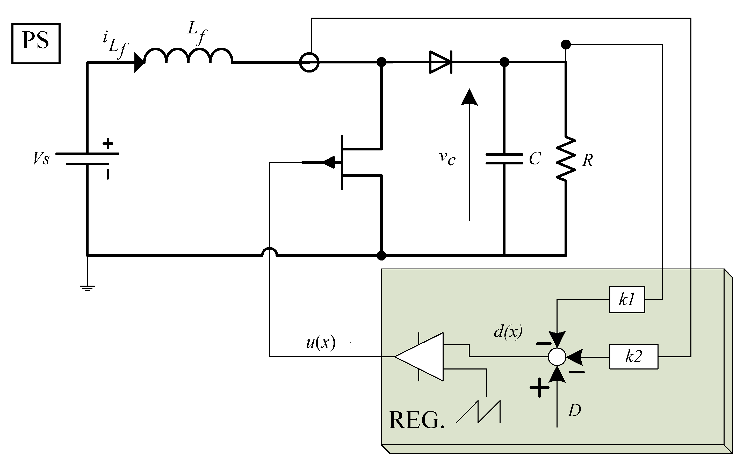
4. Numerical and Experimental Results for a Largely Used Power Electronic Converter Topology and Discussion

The theoretical results obtained in the previous sections find wide and relevant applications in the field of power electronics. In order to show their relevance for this branch of engineering, in the following, they are applied to a converter topology widely used in various engineering sectors, by electric vehicles and in general of sustainable mobility field to the renewable energy field: the boost converter. It is a PEC characterized by a system of ODE of the second order discontinuous right-hand side which, powered by a constant voltage vs. at the input, provides at the output a constant voltage v_c, whose value is theoretically adjustable within the set [V_s, +$\infty$[. The electrical circuit of a boost converter with the associated system control is shown in Figure 1.

It consists of two blocks: the Power Stage (PS) block and the Regulator (Reg) block. The PS block is made up of a battery V_s, an inductor L_f, a capacitor C, a controlled component M and a diode D. It is a part dedicated to converting electrical energy at voltage vs. into electrical energy at voltage v_c.

The “Reg” block of the controller measures the state variables (the current in the inductor L_f and the voltage across the capacitor C) and calculates the duty ratio d(x) necessary so that the output voltage v_c goes from the actual value to the desired one within the range [V_s, +$\infty$[.

It implements the following relation:

$$d\left(x\right)=D-k_1{x}_{1,n}-k_2{x}_{2,n}.$$

The duty ratio represents the average value, calculated on each period T_s, of the u(x) signal to be applied to the controlled component at each switching period T_s. The signal u can take values only in the discrete set $\left\{0,1\right\}$. It is 1 when the component is switched to conduction, and zero when the component is opened. The “PWM” block of the controller is deputed to transform the duty ratio d(x) in the signal u(x). It implements the following relation:

$$u=H\left(d\left(x\right)-tri\left(t_n,1\right)\right)$$

where H represents the Heaviside function.

The differential system of equations representing a boost converter is the following:

$$\frac{d}{d{t}_n}x={\mathsf{\epsilon }}_0\left[f_0\left(x\right)+f_1\left(x\right)u\right]$$

with:

$$\begin{array}{l}{\mathsf{\tau }}_1=\frac{L_f}{R}; {\mathsf{\tau }}_2=RC; {\mathsf{\epsilon }}_1=\frac{T}{{\mathsf{\tau }}_1};{\mathsf{\epsilon }}_2=\frac{T}{{\mathsf{\tau }}_2}; t_n=\frac{t}{T}\\ {\mathsf{\epsilon }}_0=\frac{T}{\min \left\{{\mathsf{\tau }}_1,{\mathsf{\tau }}_2\right\}}=\max \left\{{\mathsf{\epsilon }}_1,{\mathsf{\epsilon }}_2\right\}; x_{1,n}=\frac{R{i}_{L_f}}{V_s}; x_{2,n}=\frac{v_C}{V_s};\\ f_0\left(x\right)=\frac{1}{{\mathsf{\epsilon }}_0}\left(\begin{array}{l}{\mathsf{\epsilon }}_1\left(1-x_{2,n}\right)\\ {\mathsf{\epsilon }}_2\left(x_{1,n}-x_{2,n}\right)\end{array}\right);f_1\left(x\right)=\frac{1}{\mathsf{\epsilon }}\left(\begin{array}{l}{x}_{2,n}{\mathsf{\epsilon }}_1\\ -x_{1,n}{\mathsf{\epsilon }}_2\end{array}\right);\\ x={\left[x_{1,n},x_{2,n}\right]}^t\end{array}$$

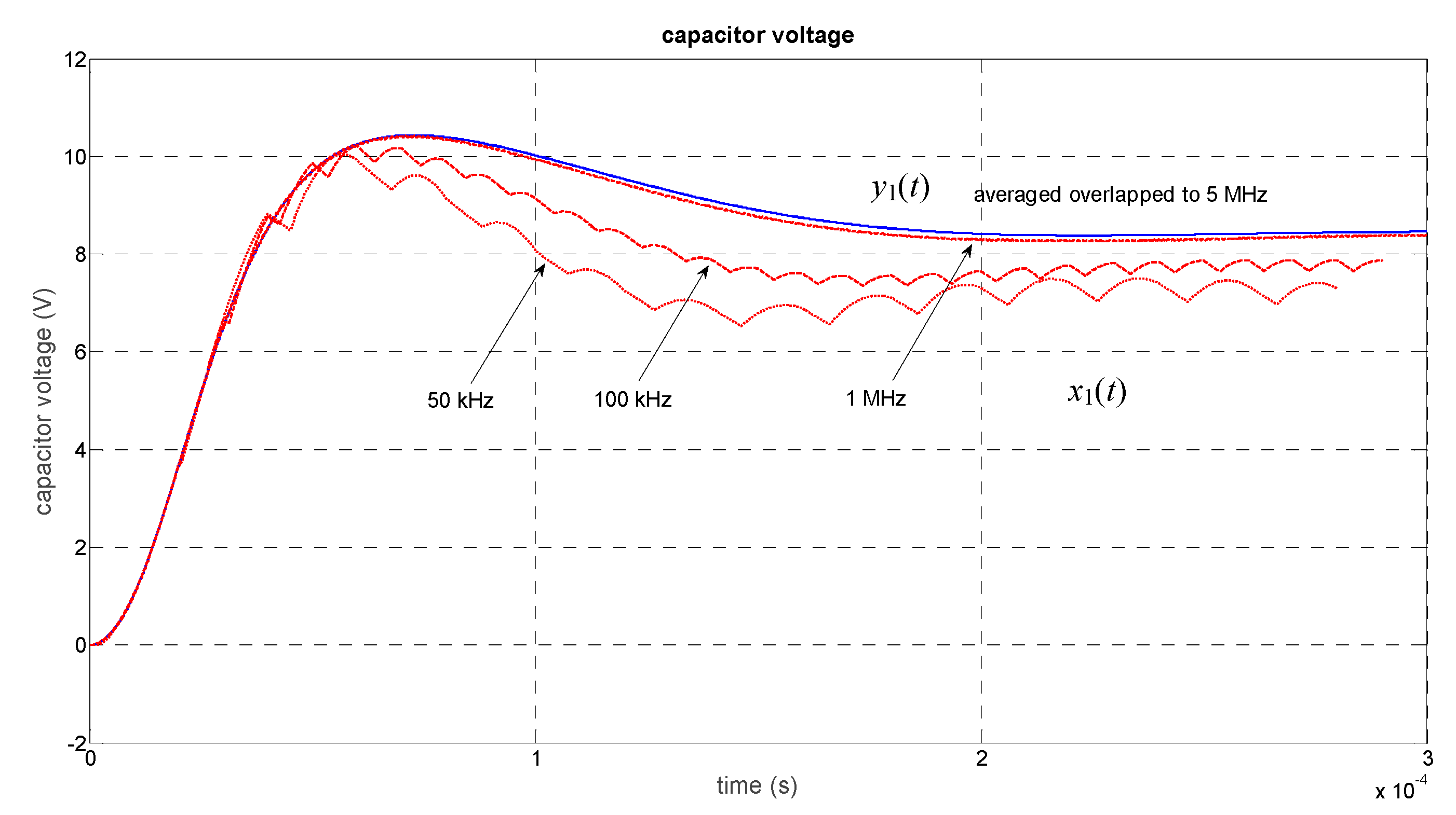
In order to provide an application of relation (18), the operation of the boost converter having the parameters reported in

Table 1. Electrical Parameters of the Boost Converter.

Parameter	Converter
Lf	50 μH
C	4.39 μF
R	27.9 Ω
K1	0.1739
K2	−0.0435
Vs	5 V
Vref	8.5 V

with different switching periods was simulated.

The error in the desired norm was set at 0.3. The application of the relation (18) has given a period $T_{\mathsf{\eta }}=1.00 \mu s$ as the maximum period that verifies the desired error. The circuit of Figure 1 was simulated with the switching periods shown in

Table 2. Desired Error η = 0.3.

ηe,max	T (μs)
0.0785	0.20
0.2840	1.00
2.630	10.00
4.940	20.00

. In this table, it is noted that, for switching periods belonging to the interval set by (18), i.e., ]0, T_η[, the error is lower than the desired one, as envisaged by the relation (18), while for periods not belonging to this range, the error is greater. In Figure 2, a numerical validation of (22) is shown. The different curves show the trend of the output voltage for different switching periods. As can be seen from Figure 2, as the switching period decreases (or if it is equivalent to the increase in the switching frequency) the trend of the integral curve of x_T tends to approach the trend of the integral curve of y (the top waveform in Figure 2), showing the uniform convergence of the x_T versus y.

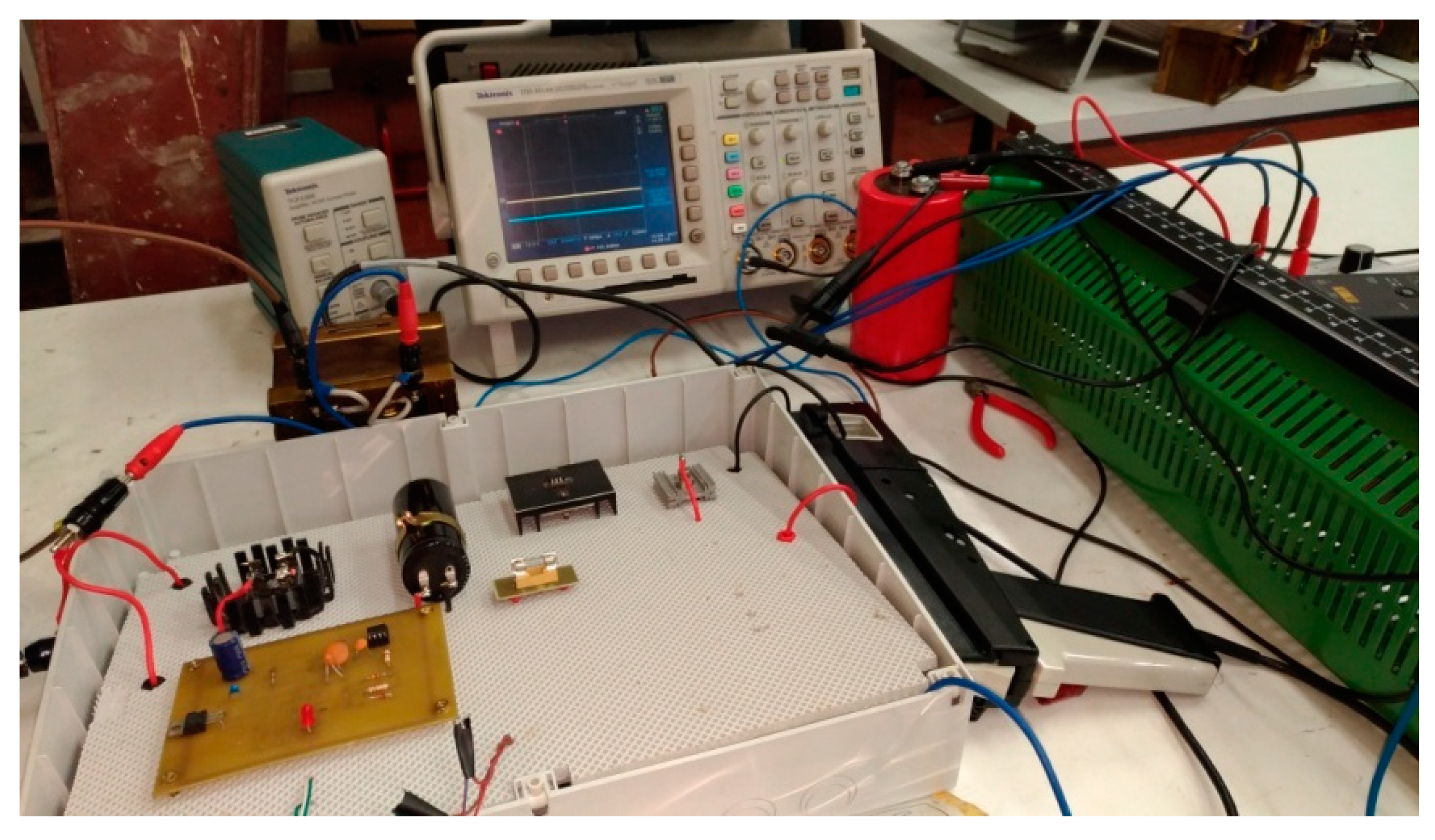
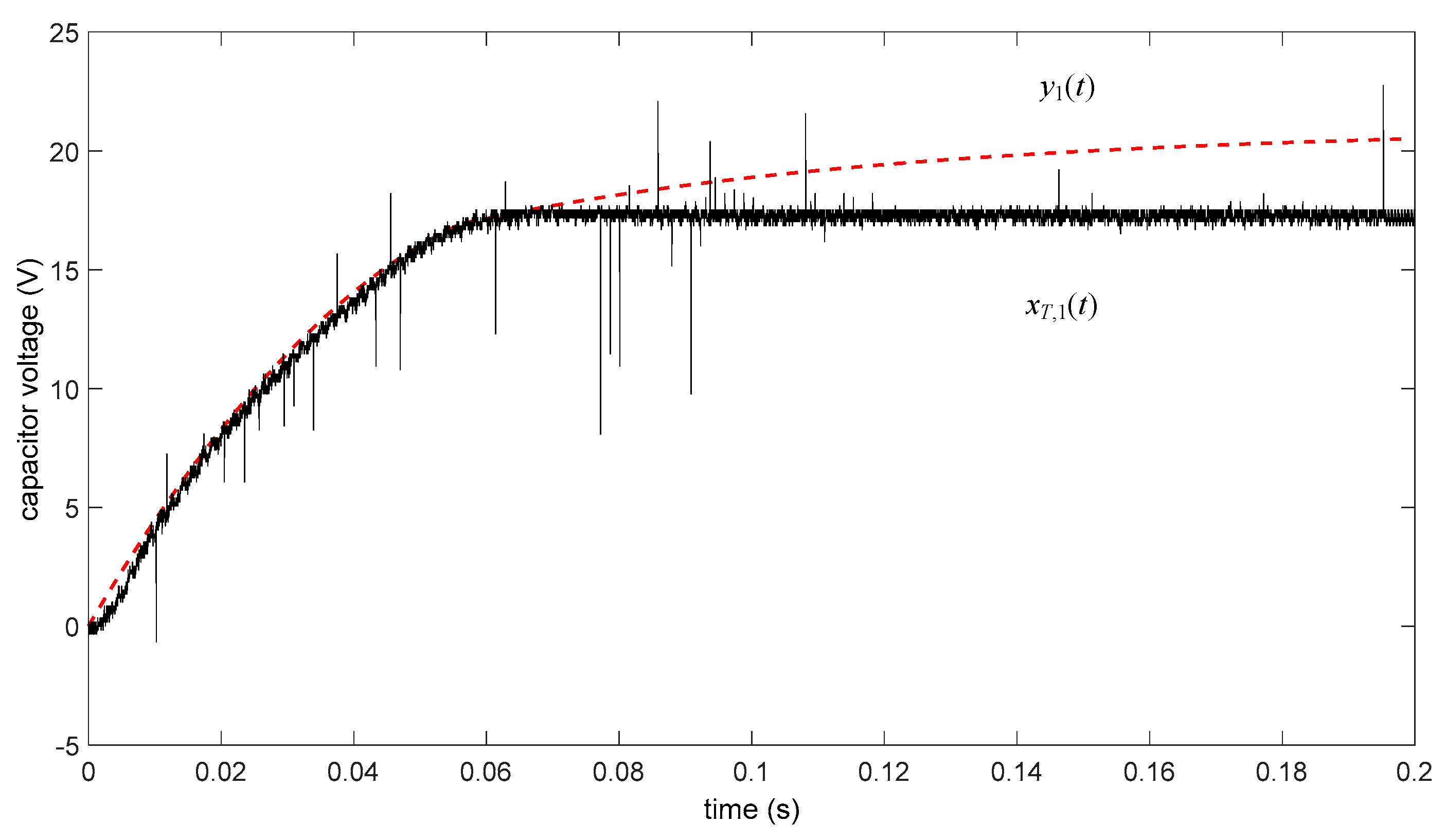
Similar results were obtained on a laboratory-made prototype of a boost converter, as shown in Figure 3.

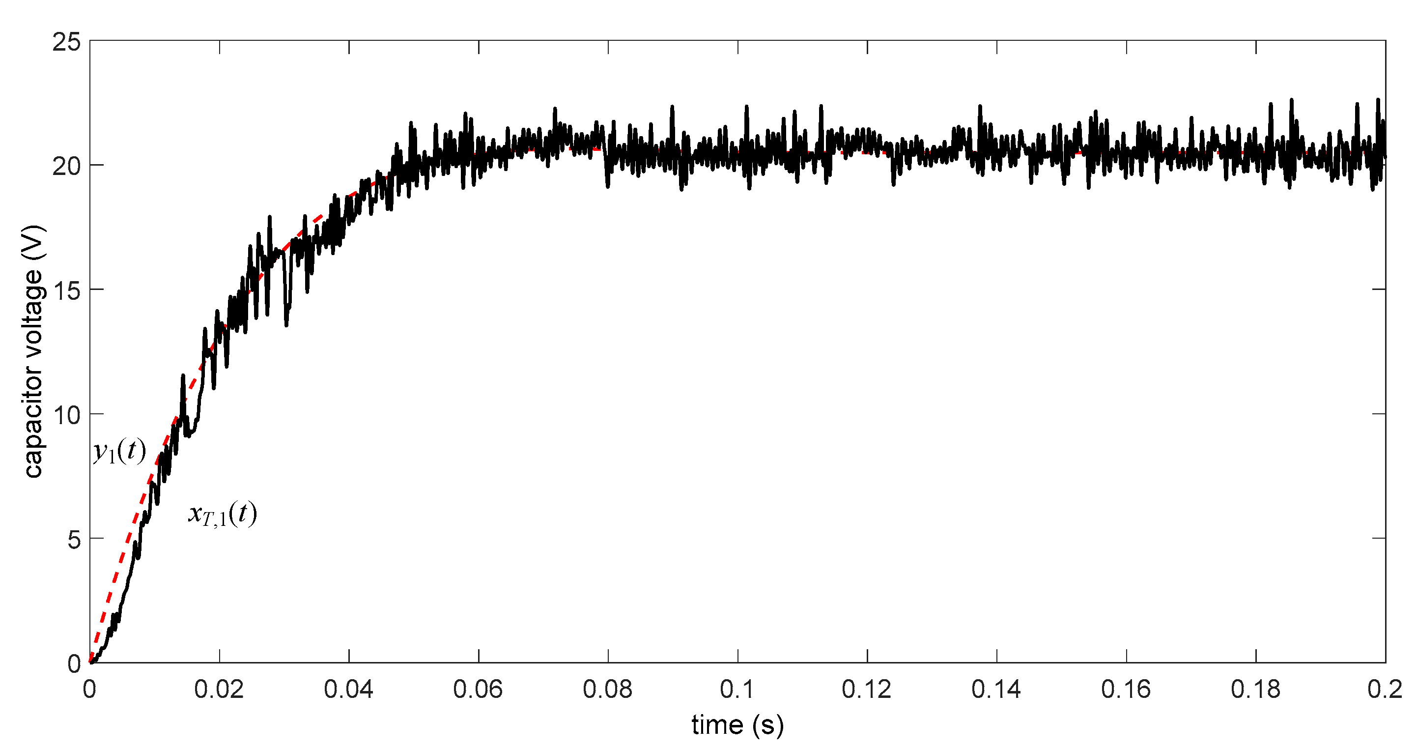
A desired error in the norm of 0.8 was set and, from the relation (18), we obtained T_η = 70 $\mathsf{\mu }\mathrm{s}$. The converter was made to work with two different switching periods, T₁ = 60 $\mathsf{\mu }\mathrm{s}$ and T₂ = 1.52 ms. The results reported in Figure 4 and Figure 5 were obtained. As can be seen from the figures, working with the switching period T₁ lower than T_η (Figure 4), the two solutions overlap, while in the case of Figure 5, the waveforms move away presenting an error greater than the desired one.

The physical explanation of these trends represented mathematically by the relations (18) and (22) is evident: the averaged method provides information on the time evolution of the moving average of the components of the state vector, not on the evolution of the instantaneous values of these components. Therefore, the larger the evolution time constants of the state vector components are, compared to the switching period, the more the quantities vary little, within the switching period between the beginning and the end of the period and, therefore, the better the moving average of the quantities approximates the instantaneous values in each period. This explains why, by increasing the frequency, i.e., reducing the period, the actual waveforms tend to the averaged model. This also explains why, by increasing the switching period, the standard error between the solution of the actual model and the one of the averaged model increases.

The advantages of this method compared to other ones present in the literature are different: it is a simple method to apply, it provides the possibility of formulating simple control algorithms, and it leads, in the case of open loop controls, to a system of ordinary differential equations that can be resolved also analytically in some converters.

Compared to the latest results obtained on the subject [28,29], which demonstrated only a uniform convergence of y(t) to x_T(t) as the switching period tends to zero, first of all, this work provides a proof of existence and uniqueness in the sense of Filippov to the problem of determining the temporal evolution of the quantities of a converter and it also provides formulas for calculating the error that is committed in using the approximate solution found with the averaged method instead of the exact one.

5. Conclusions

The paper analyzes a class of time-varying systems very common in the engineering field: the class of power electronic converters. This class can be represented with a system of ordinary differential equations discontinuous right-hand side which has the property of non-chattering. By exploiting this property, the paper demonstrates the existence and the uniqueness of a global solution in Filippov’s sense, for the Cauchy problem related to such system of ordinary differential equations. Furthermore, using the averaging method, the system of differential equations discontinuous right-hand side is re-formulated into a system of ordinary differential equations that admits a unique solution according to the Cauchy-Lipschitz theorem. The paper demonstrates that, under appropriate hypotheses, this approximate solution converges uniformly to the solution of the original system. Finally, relationships of considerable importance are provided for the control and the analysis of the power converters, which allow calculating the error in norm between the two solutions. The demonstrations are also supported by experimental evidence. The need to improve the approximation of the proposed formula—the formula which provides the normal error between x and y, distinguishing between stable and unstable systems—remains a problem. Additionally, what information the stability conditions of the averaged model provides, with respect to the stability conditions of the actual model, remains to be understood.

References

1. Banerjee, S.; Verghese, G. Nonlinear Phenomena in Power Electronics: Attractors, Bifurcations, Chaos and Nonlinear Control; Wiley & Sons: Hoboken, NJ, USA, 2001; ISBN 0780353838. [Google Scholar]
2. Fatou, P. Sur le mouvement d’un système soumis à des forces à courte période. Bull. Société Mathématique Fr. 1928, 2, 98–139. [Google Scholar] [CrossRef] [Green Version]
3. Mandelstam, L.I.; Papalexi, N.D. Uber die Begründung einer Methode für die Näherungslösung von Differentialgleichungen. J. F Exp. Phys. 1934, 4, 117. [Google Scholar]
4. Krylov, N.M.; Bogoliubov, N.N. Introduction to Nonlinear Mechanics; Patent No. 1; Kiev, Ukraine, Izd. Akad. Nauk. Sssr 1937; Translated in English by S. Lefschetz; Introduction to non-linear mechanics; Princeton University Press: Princeton, NJ, USA, 1943. (In Russian) [Google Scholar]
5. Bogoliubov, N.N.; Mitropolskii, Y.A. Asymptotic Methods in the Theory of Nonlinear Oscillations; Gordon and Breach: New York, NY, USA, 1961. [Google Scholar]
6. Roseau, M. Vibrations Nonlinéaires et Théorie de la Stabilité; Springer: Berlin/Heidelberg, Germany, 1966. [Google Scholar]
7. Besjes, J.G. On the asymptotic methods for non-linear differential equations. J. Mécanique 1969, 8, 357–373. [Google Scholar]
8. Perko, L.M. Higher Order Averaging and Related Methods for Perturbed Periodic and Quasi-Periodic Systems. Siam J. Appl. Math. 1969, 17, 698–724. [Google Scholar] [CrossRef]
9. Banfi, C. Sull’approssimazione di processi non stazionari in meccanica non lineare. Bolletino Dell Unione Mat. Ital. 1967, 22, 442–450. [Google Scholar]
10. Banfi, C.; Graffi, D. Sur les methodes approchées de la mécanique non linéaire. Actes Du Coll. Equ. Diff. Non Lin 1969, 1, 33–41. [Google Scholar]
11. Eckhaus, W. New approach to the asymptotic theory of nonlinear oscillations and wave-propagation. J. Math. Anal. Appl. 1975, 49, 575–611. [Google Scholar] [CrossRef] [Green Version]
12. Buică, A.; Llibre, J. Averaging methods for finding periodic orbits via Brouwer degree. Bull. Sci. Mathématiques 2004, 128, 7–22. [Google Scholar] [CrossRef] [Green Version]
13. Kruzweil, J. The averaging principle in certain special cases of boundary problems for partial differential equations. Cas. Pst. Mat. 1963, 88, 444–456. [Google Scholar]
14. Meerkov, S.M. Averaging of trajectories of slow dynamic systems. Differ. Equ. 1973, 9, 1239–1245. [Google Scholar]
15. Mesquita, J.G.; Slavík, A. Periodic averaging theorems for various types of equations. J. Math. Anal. Appl. 2012, 387, 862–877. [Google Scholar] [CrossRef]
16. Morrison, J.A. An Averaging Scheme for Some Nonlinear Resonance Problems. Siam J. Appl. Math. 1968, 16, 1024–1047. [Google Scholar] [CrossRef]
17. Plotnikov, V.A. Averaging methods for differential inclusions and its applications to optimal control problems. Differ. Equ. 1979, 15, 1013–1018. [Google Scholar]
18. Sanders, J.; Verhulst, F. Averaging method in nonlinear dynamical systems. In Applied Mathematical Sciences; Springer: Berlin/Heidelberg, Germany, 1985. [Google Scholar]
19. Sethna, P.R. An extension of the method of averaging. Q. Appl. Math. 1967, 25, 205–211. [Google Scholar] [CrossRef] [Green Version]
20. Llibre, J.; Novaes, D.D.; Teixeira, M.A. On the periodic solutions of a generalized smooth and nonsmooth perturbed planar double pendulum with small oscillations. arXiv 2012, arXiv:1203.0498v1. [Google Scholar]
21. Cardin, P.T.; De Carvalho, T.; Llibre, J. Limit Cycles of Discontinuous Piecewise Linear Differential Systems. Int. J. Bifurc. Chaos 2011, 21, 3181–3194. [Google Scholar] [CrossRef] [Green Version]
22. Llibre, J.; Rong, F. On the Number of Limit Cycles for Discontinuous Piecewise Linear Differential Systems in ℝ2n with Two Zones. Int. J. Bifurc. Chaos 2013, 23, 1350024. [Google Scholar] [CrossRef] [Green Version]
23. Kunze, M. Non-Smooth Dynamical Systems, Lecture Notes in Math; Springer: Berlin/Heidelberg, Germany, 1744. [Google Scholar]
24. Wiercigroch, M.; de Kraker, B. Applied Nonlinear Dynamics and Chaos of Mechanical Systems with Discontinuities; World Scientific Publishing: Hackensack, NJ, USA, 2000. [Google Scholar]
25. Vázquez-Polo, F.-J.; Negrín-Hernández, M.-Á.; Martel-Escobar, M. Meta-Analysis with Few Studies and Binary Data: A Bayesian Model Averaging Approach. Mathematics 2020, 8, 2159. [Google Scholar] [CrossRef]
26. Moreno-Pulido, S.; García-Pacheco, F.; Sánchez-Alzola, A.; Rincón-Casado, A. Convergence Analysis of the Straightforward Expansion Perturbation Method for Weakly Nonlinear Vibrations. Mathematics 2021, 9, 1036. [Google Scholar] [CrossRef]
27. Walsh, J.; Widiasih, E. A Discontinuous ODE Model of the Glacial Cycles with Diffusive Heat Transport. Mathematics 2020, 8, 316. [Google Scholar] [CrossRef] [Green Version]
28. Krein, P.; Bentsman, J.; Bass, R.; Lesieutre, B. On the use of averaging for the analysis of power electronic systems. IEEE Trans. Power Electron. 1990, 5, 182–190. [Google Scholar] [CrossRef]
29. Lehman, B.; Bass, R.M. Extensions of averaging theory for power electronic systems. IEEE Trans. Power Electron. 1996, 11, 542–553. [Google Scholar] [CrossRef] [Green Version]
30. Meyer, K.R. Ordinary Differential Equations (Jack K. Hale. John Wiley). Siam Rev. 2006, 14, 348–350. [Google Scholar] [CrossRef]
31. Filippov, A. Differential Equations with Discontinuous Right-hand-Sides. Am. Math. Soc. Trans. 1964, 42, 199–231. [Google Scholar]
32. Meo, S.; Toscano, L. Some New Results on the Averaging Theory Approach for the Analysis of Power Electronic Converters. IEEE Trans. Ind. Electron. 2018, 65, 9367–9377. [Google Scholar] [CrossRef]
Figure 1. Circuital schema of a PWM controlled boost converter.
Mathematics 09 01146 g001
Figure 2. Transient of the voltage component x1(t) of xT and y1(t) of y(t).
Mathematics 09 01146 g002
Figure 3. PWM controlled dc-dc boost converter prototype.
Mathematics 09 01146 g003
Figure 4. Transient of the voltage component x1(t) of xT and y1(t) of y(t) for T = 60 μ s .
Mathematics 09 01146 g004
Figure 5. Transient of the voltage component x1(t) of xT and y1(t) of y(t) for T = 1.52 ms.
Mathematics 09 01146 g005